Risk Coupling Analysis of Deep Foundation Pits Adjacent to Existing Underpass Tunnels Based on Dynamic Bayesian Network and N–K Model

Abstract

Because deep foundation pits and tunnels are deformation-sensitive structures, the safety of these projects is generally affected by coupled risks. In deep foundation pit construction, if the existing tunnel structure adjacent to the deposit is damaged, it can produce a severe group disaster. It is necessary to identify an efficient risk analysis model to study the dynamic coupled risk of deep foundation pit projects adjacent to existing underpass tunnels and to analyze the risk evolution law to achieve effective real-time safety control. This study proposes a coupled risk analysis model using the N–K model and dynamic Bayesian network to construct deep foundation pits in adjacent existing underpass tunnels. The model is predicated on association rules to explore the interrelationship between risk factors to build a dynamic Bayesian network structure. In addition, the N–K model is utilized to quantify coupled risks under such complex working conditions and to optimize the dynamic Bayesian network structure. The developed model clarifies the risk coupling mechanism of deep foundation pit construction adjacent to an existing underpass tunnel, finds the critical points in the risk transfer process, and conducts dynamic risk prediction and accident causation diagnosis for the coupled risk to realize the dynamic control of the coupled risk in the adjacent existing underpass tunnel construction. Taking the Nanning underground comprehensive utilization project as an example, the validity and applicability of the proposed approach were tested. The results showed that the model is feasible and has application potential, providing effective decision support for safety control while constructing deep foundation pits adjacent to existing tunnels.

1. Introduction

The deep foundation pit projects in the city are often surrounded by buildings, underground pipelines, subway tunnels, and others [1]. The excavation of deep foundation pits (DFPs) redistributes the groundwater level and stresses in the soil, changing the soil’s original stress state, and negatively impacting the adjacent buildings, pipelines, and subway tunnels [2]. Therefore, the study of the effect of the foundation pit excavation process on the surrounding environment, especially on the adjacent existing subway tunnel, should not only consider the strength and stability of the foundation pit support itself, but also monitor and control its deformation to prevent harm to the normal use of the subway tunnel.

The safety of DFP construction adjacent to existing underpass tunnels is subject to various risk factors. There is a coupling effect between risk factors, which will have a sudden, irreversible nonlinear impact on the whole DFP construction system, leading to an increase in the probability of occurrence of the risk and an increase in the severity of accident consequences, and this coupling risk will change to different degrees with the changes in coupling factors [3]. Although previous studies have analyzed the occurrence and evolution mechanism of the safety risk of construction accidents adjacent to existing underpass tunnels, the coupling mechanism within the evolution mechanism has received insufficient attention. Engineers only recognize the process and impact of a single risk in time and space, and ignoring the different kinds of safety risks in which a coupling effect can also occur increases the probability of dangerous accidents.

Many scholars have carried out many related studies on similar geotechnical problems, resulting in numerous accomplishments. For instance, Wei et al. [4] used machine learning models to predict the compressive strength of rocks and provide new insights into the rate-dependent strength of rocks. Zhang et al. [5] developed a new intelligent optimized back-analysis method, PSO-GP-FDM, to obtain the mechanical properties of the surrounding rocks of underground cavern groups. However, numerical simulation is still the most common method. In practical engineering, it is inevitable to encounter a substantial numerical simulation workload, affecting the timeliness of engineering decisions [6]. In addition, other traditional risk analysis methods have many limitations. For example, fuzzy hierarchical analysis (FAHP) is too cumbersome in the calculation process for the complex evaluation of multiple factors and levels [7]. Fault tree analysis (FTA) does not permit dynamic risk analysis [8,9,10]. For support vector machines (SVMs), the parameters are usually obtained by manual trials, often with a certain degree of subjectivity and blindness [11]. Neural networks (NNs) suffer from over-fitting problems [12]. Uncertainty is unavoidable when assessing and diagnosing the risk associated with deep foundation construction adjacent to existing underpass tunnels. Bayesian networks are a powerful tool for expressing uncertainty knowledge and reasoning about uncertainty, they have been widely used in reliability and risk analysis in many fields [13], and can compensate to some extent for the limitations of the above-mentioned traditional methods. For example, Wu et al. [8] suggested that the relevant influencing factors are changing with the progress of shield construction. They developed a model for dynamic risk analysis using dynamic Bayesian networks (DBN) to support safety analysis in tunnel construction. Evaluating the risk of DFP construction adjacent to existing underpass tunnels also needs to consider the dynamic changes of influencing factors. However, the current dynamic Bayesian network (DBN) does not consider the coupling relationship between risk factors and cannot realize the dynamic control of coupled risks. The dynamic Bayesian network produces poor classification results when dealing with small probability risks [14]. Therefore, for building DFPs adjacent to existing underpass tunnels, a complex project that has not yet formed a mature management model, it is urgent to find an effective risk analysis model, conduct research on its dynamic coupled risk, analyze the law of risk evolution, and take efficient measures to achieve dynamic risk control.

Several mathematical models are utilized to measure coupling risk. Among them, the coupling degree model refers to the use of the expert scoring method to obtain quantitative data, which has certain limitations. The interpretative structural modeling method is easily affected by the internal factors of the system, and the primary and secondary hierarchical relationship of the system cannot be clarified, while the algorithm of the nonlinear dynamic model is too complex [15]. Because the N–K model adopts mathematical and statistical methods by applying objective accident statistics to measure the coupled risk between factors and thereby avoiding the influence of subjective factors, it has been widely accepted by scholars [16]. However, research on the coupled risk of construction accidents in DFPs adjacent to existing underpass tunnels is still lacking. Based on a large number of existing underpass tunnels and DFP construction site monitoring data, association rule mining (ARM) can discover unknown strong correlations and rules implied in the large dataset (i.e., correlations between risk factors). In particular, the combination of risk factors with a low probability of occurrence but strong correlation can provide a basis for risk dynamic analysis and assessment. Consequently, this study introduces the N–K model and DBN into the field of construction risk assessment of DFPs adjacent to existing underpass tunnels for the first time and proposes a new coupled risk dynamic analysis model. The model constructs a dynamic Bayesian network structure that relies on the interrelationship of risk factors obtained by association rule mining and optimizes the dynamic Bayesian network structure using the N–K model to compensate for the shortcomings of Bayesian networks. The model can diagnose and predict the dynamic risk during the construction of DFPs adjacent to existing underpass tunnels, and the method’s effectiveness and feasibility were verified by analyzing the underground space utilization project from Guangxi University Station to Guangxi Finance and Economics College of Nanning Rail Line 5 as an example.

2. Methodology

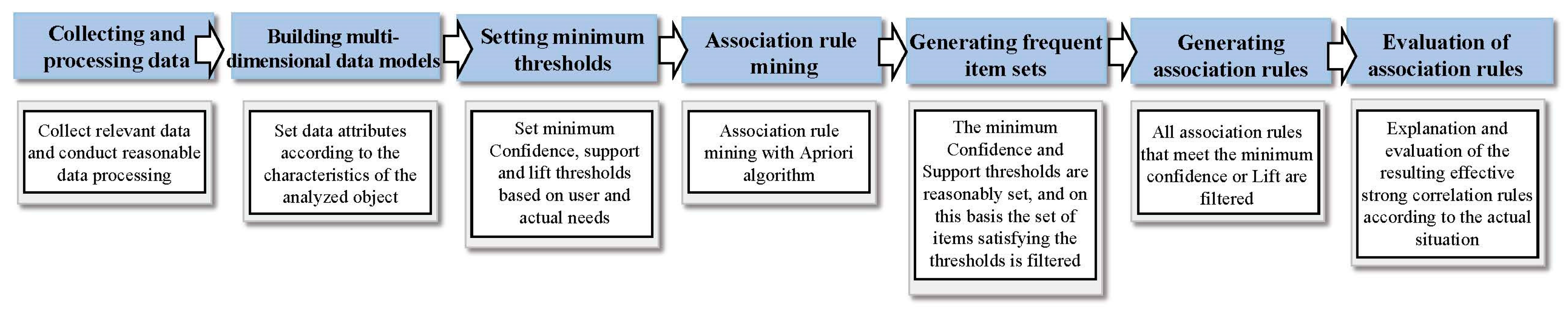
2.1. Risk Association Analysis and Apriori Algorithm

Currently, association rules mining is considered as an important technique for extensive data analysis, mainly used to mine valuable correlations between data [17].

2.1.1. Relevant Concepts of Association Rules

Definition 1.

(Association Rules): Let $I=\left\{i_1,i_2,\cdots i_n\right\}$ be the set of all items, while P is a subset of I, $\left\{P=\left\{i_j,\cdots i_k\right\}\subseteq I,1\le j,k\le n\right\}$ . Then, the following type of association rules can be defined as follows:

$$IFAntecedentTHENConsequent\left(A\Rightarrow C\right)$$

(1)

where both the Antecedent (A) and Consequent (C) are subsets of P.

Definition 2.

(Support): The support of association rule A ⇒ C is the percentage of transactions containing sets A and C among all transaction items, as shown in Equation (2), and the support can be understood as the frequency of the association rule.

$$Support\left(A\Rightarrow C\right)=\frac{\left|\left\{T:A\cup C\subseteq T,T\subseteq D\right\}\right|}{\left|D\right|}$$

(2)

Definition 3.

(Confidence): The confidence level of association rule A ⇒ C is the percentage of transactions containing sets A and C among all transactions containing item set A, as shown in Equation (3), and the confidence level can be understood as the strength of the association rule.

$$Confidence(A\Rightarrow C)=\frac{\left|\left\{T:A\cup C\subseteq T,T\subseteq D\right\}\right|}{\left|\left\{T:A\subseteq T,T\subseteq D\right\}\right|}=\frac{Support\left(A\Rightarrow C\right)}{Support\left(A\right)}$$

(3)

It should be noted that a threshold is typically required to filter the association rules as follows [18]:

1. 

Minimum support: the minimum support that the association rule must statistically satisfy.

2. 

Minimum confidence: the minimum confidence level that the association rule must statistically satisfy.

The support and the confidence are widely considered as good measures of the association rules’ relevance in ARM, but exceeding the minimum threshold does not guarantee that the rules are valid, and the assessment of the support and the confidence as importance and accuracy measures of association rules have several drawbacks. In order to obtain a valid association rule from a strong one, another important metric known as the lift [19] can be used for filtering.

Definition 4.

(Lift): The lift of association rule A ⇒ C is the percentage of observed support to expected support when A and C are independent, as shown in Equation (4). It indicates the validity and importance of association rule A ⇒ C.

$$Lift(A\Rightarrow C)=\frac{Supp(A\cup C)}{Supp\left(A\right)\times Supp\left(C\right)}$$

(4)

The lift refers to the dependency between the antecedent and consequent of an association rule. If the lift exceeds 1, C is likely to be highly correlated with A, which means that the association rule may be useful for predicting future outcomes in the dataset. Therefore, it can help filter and obtain valid results [3].

2.1.2. Apriori Algorithm and Association Rule Mining

The Apriori algorithm is the most commonly used algorithm for association rule mining, which has a wide range of applications [20]. The main steps of association rule mining using the Apriori algorithm are shown in Figure 1 [21]:

2.2. Theory of Dynamic Bayesian Networks

2.2.1. Dynamic Bayesian Network (DBN)

A Bayesian network is a directed acyclic graph consisting of nodes, directed arcs, and prior and conditional probabilities [22]. The nodes in a Bayesian network are represented by a random variable $(X_1,\dots ,X_N)$. Assuming that Par(Xi) is the probability of occurrence of node Xi at the parent node in the model, the conditional probability of node Xi can be expressed as $P(X_i|Pa(X_i))$, and the joint probability distribution $P(X_1,\dots ,X_N)$ can be defined as follows:

$$P(X_1,\dots ,X_N)={\displaystyle \prod _{i=1}^{\mathrm{n}}P(X_i|P_{ar}(X_i))}$$

(5)

Bayesian networks can perform both forward (predictive) and backward (diagnostic) analysis, and the posterior probability of any variable can be obtained by inference. Inference in Bayesian networks is the calculation of probabilities for an unknown variable in the presence of known ones. Knowing the variable Y, the conditional probability of X is as follows:

$$P(X|Y)=\frac{P(X)P(Y|X)}{P(Y)}$$

(6)

A dynamic Bayesian network is a probabilistic model that can process time-series data by fusing the original network structure and temporal information based on a static Bayesian network. In order to simplify the modeling of complex systems, simple assumptions and conditions are applied to the model [23]:

(1)

Smoothness assumption: Assuming that the network topology does not change over time, the probability change process of the variables is uniformly smooth over a finite time t (i.e., the conditional probability $P(X_i|Pa(X_i))$ remains constant for all t).

(2)

Markov assumption: Given the state at the current moment t, the state at the future moment t + 1 is only related to the state at moment t and not to the state at the moment t + 1, as expressed by the following equation:

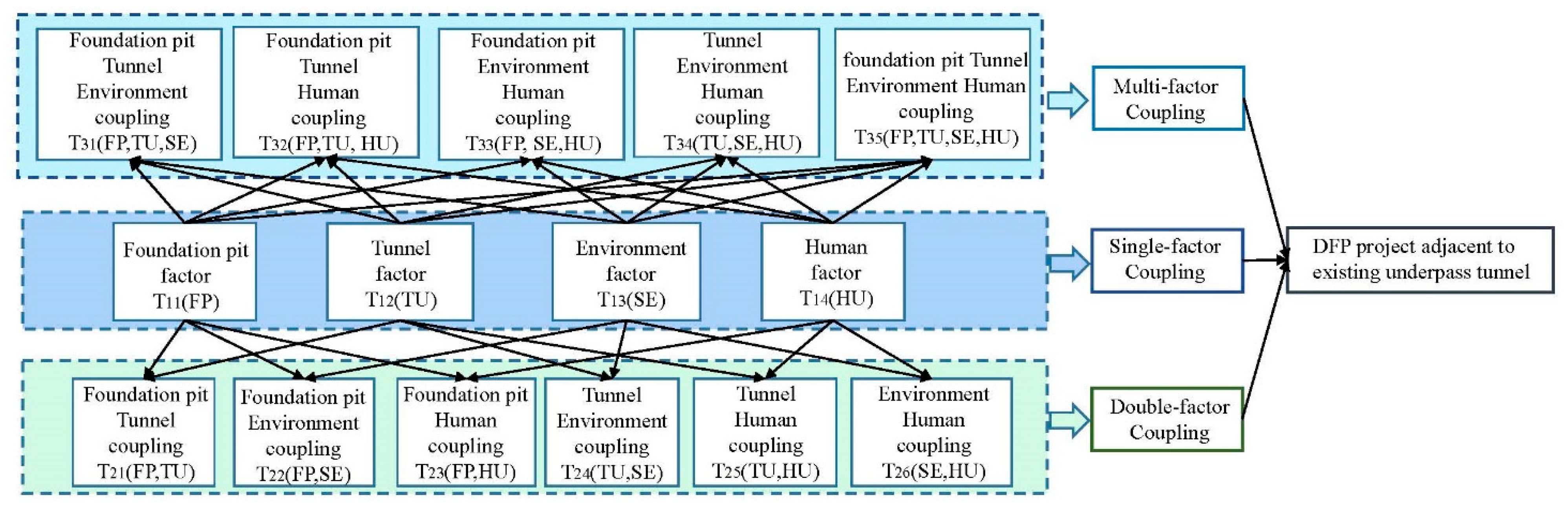
$$P(X^{t+1}/X^0,\cdots ,X^t)=P(X^{t+1}/X^t)$$

(7)

Based on the above assumptions, the dynamic Bayesian network is defined as $(B_1,B_{\to })$, where the Bayesian of the initial moment is represented by $B_1$, and the combined Bayesian network graphs on different time slices are represented by $B_{\to }$. By expanding the dynamic Bayesian network to the Tth time slice and using the initial probability distribution and the conditional probability distribution between adjacent time slices, the joint probability distribution across multiple time slices can be obtained as follows:

$$P(X_{1:T})=\stackrel{T}{\prod _{t=1}}\stackrel{N}{\prod _{i=1}}P(X_t^i|P_{ar}(X_t^i))$$

(8)

2.3. N–K Model

The N–K model is a model proposed by Kauffman in his study of the evolution of biological and genetic assemblages that uses N and K to describe the degree of complexity of the associations between subjects in a system [24]. The N–K model describes the role of node interdependence in complex adaptive systems [25], where N is the number of elements that make up the system and K is the number of interacting and coupled elements in the system. Each element has n states; hence there are n^N possible coupling methods, where K is at least 0 and at most N − 1. The coupling degree of risk factors can be expressed using mutual information with the following equation [16,26]:

$$T(X_1,\cdots ,X_i)={\displaystyle \sum _{x_1}^{}\cdots {\displaystyle \sum _{x_i}p(X_1,\cdots ,X_i)\times {\log }_2(p(X_1,\cdots ,X_i)/p(X_1)\cdots p(X_i))}}$$

(9)

where $X_i$ is the ith element; $p(X_1,\cdots ,X_i)$ is the probability that the element coupling occurs; and $p(X_i)$ is the probability that the ith element is in a certain state.

3. Establishment of a Dynamic Analysis Model for Coupled Risk Analysis of DFPs Adjacent to Existing Underpass Tunnels Based on DBN and N–K Models

The framework for constructing a dynamic Bayesian network process that predicts the probability of construction accidents in DFPs adjacent to existing tunnels is shown in Figure 2 with the following steps:

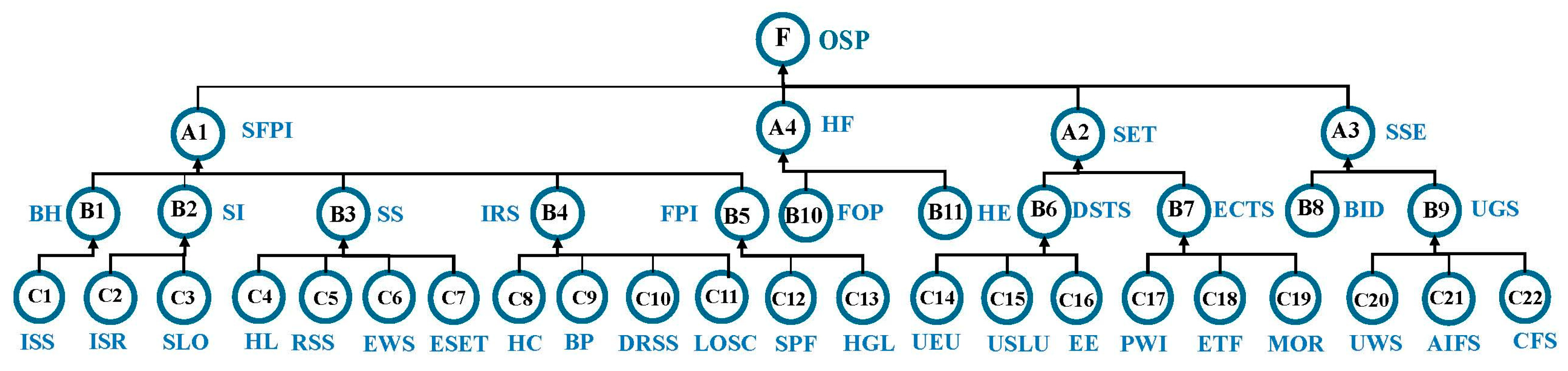
3.1. Identification of Risk Factors and Bayesian Network Nodes

Risk identification is an ongoing and complex process that includes identifying specific risk events in the project as well as identifying risk categories and possible risk factors. In this study, the expert survey method and Dempster–Shafer evidence theory were initially used to determine the risk factors. The survey included the factors affecting the overall safety of DFP projects adjacent to existing underpass tunnels and the methods for quantifying the risk factors. Through risk identification, the risk factors affecting the DFP project adjacent to the existing underpass tunnel are identified, and their risk status levels are also determined, among which, for the risk level of the overall project risk, experts need to assess the overall project risk through the amount of the enclosure pile’s lateral movement, the amount of ground settlement, and the relevant monitoring values of the existing tunnel. As long as any item appears abnormal, the overall project safety is considered low, and the risk potential is high. However, due to the engineering complexity, numerous risk factors are identified, and redundancy often occurs, affecting the efficiency of risk assessment. Accordingly, it is necessary to use the Apriori algorithm to mine risk correlation and select key factors affecting engineering risk.

The collected sample data must be discretized and filtered before performing the risk correlation analysis. In the process of association rule mining for DFP construction risk adjacent to existing underpass tunnels, the confidence results of the generated association rules are very close, so the confidence level cannot be used as a useful threshold for filtering association rules. Therefore, this paper selected the minimum support degree and the lifting degree to filter and generate effective association rules, especially using the lifting degree to pick out the factors that have a greater impact on the overall risk. After setting the minimum threshold, the set of frequent items satisfying the minimum support is filtered using the Apriori algorithm. The risk factors can describe the occurrence and development of pit construction accidents in the obtained frequent item set. Thus, these risk factors are selected as nodes, and all possible values of the variables are determined.

3.2. Construction of a Coupled Risk Bayesian Network Model Structure

Using the Bayesian network for estimating the probability of construction accidents in DFPs adjacent to existing subways requires adopting the association rules obtained in the previous step, utilizing directed edges to identify the causes of the outcomes, gradually constructing a Bayesian network directed acyclic graph and using Netica, version 5.18 (Norsys software Corp., Vancouver, BC, Canada), to construct a dynamic Bayesian network model containing time series. In addition, correcting the Bayesian network based on the coupled risk’s influence degree on the overall risk is needed.

Different risk factors interact with each other, forming coupled risks in the process of risk evolution while changing the intensity and frequency of the factors. The mechanism of accident coupling occurrence in DFP projects adjacent to existing underpass tunnels is shown in Figure 3. The types of risk coupling are classified according to the attributes and quantity of risk factors, as shown in Figure 4. In this study, the N–K model was used to analyze the construction safety’s coupled risk of DFPs adjacent to existing tunnels. The basic principle herein is to calculate the mutual information value (T) between the risk of the pit itself, the risk of the existing tunnel, the risk of the surrounding environment, the risk of human factors, and other factors to measure the degree of influence of the coupling effect on the construction of the DFP adjacent to the existing underpass tunnel. The larger T indicates that the more these factors are coupled in a certain way, the greater the risk of an accident. The coupling degree T of the four-factor coupling risk is calculated as follows:

$$T_4(FP,TU,SE,HU)={\displaystyle \sum _{h=1}^H{\displaystyle \sum _{i=1}^I{\displaystyle \sum _{j=1}^J{\displaystyle \sum _{k=1}^K{p}_{h,i,j,k}\times {\log }_2(p_{h,i,j,k}/(p_{h\dots }{p}_{.i..}{p}_{..j.}{p}_{\dots k}))}}}}$$

(10)

where FP, TU, SE, and HU represent the four types of risk factors such as the stability of DFP, stability of existing tunnel, stability of the surrounding environment, and human factors, respectively; h = 1, …, H; i = 1, …, I; j = 1, …, J; k = 1, …, K; $p_{h,i,j,k}$ is the probability of coupling between the stability of the pit in state h, the stability of the existing tunnel in state i, the stability of the surrounding environment in state j, and the human factor in state k.

Most construction accidents in DFPs adjacent to existing underpass tunnels are caused by the partial coupling of risk factors, and the probability of complete coupling of risk factors leading to accidents is small. Based on the number of factors involved, the risk of safety coupling in constructing DFPs adjacent to existing underpass tunnels can be divided into single-factor coupling risk, two-factor coupling risk, and multi-factor coupling risk. Two-factor coupling risk refers to the risk caused by the interaction and influence between two risk factors affecting the safety of the construction of DFPs adjacent to existing subways, mainly including the foundation pit–tunnel coupling risk, the foundation pit–environment coupling risk, the foundation pit–human coupling risk, the tunnel–environment coupling risk, the tunnel–human coupling risk, and the environment–human coupling risk. The coupling degrees T are denoted as T₂₁ (FP, TU), T₂₂ (FP, SE), T₂₃ (FP, HU), T₂₄ (TU, SE), T₂₅ (TU, HU), and T₂₆ (SE, HU), and are calculated as follows:

$$\{\begin{array}{c}{T}_{21}(FP,TU)={\displaystyle \sum _{h=1}^H{\displaystyle \sum _{i=1}^I{p}_{h,i}{\log }_2(p_{h,i}/(p_{h\dots }{p}_{.i..}))}}\\ T_{22}(FP,SE)={\displaystyle \sum _{h=1}^H{\displaystyle \sum _{j=1}^J{p}_{h,j}{\log }_2(p_{h,j}/(p_{h\dots }{p}_{..j.}))}}\\ T_{23}(FP,HU)={\displaystyle \sum _{h=1}^H{\displaystyle \sum _{k=1}^K{p}_{h,k}{\log }_2(p_{h,k}/(p_{h\dots }{p}_{\dots k}))}}\\ T_{24}(TU,SE)={\displaystyle \sum _{i=1}^I{\displaystyle \sum _{j=1}^J{p}_{i,j}{\log }_2(p_{i,j}/(p_{.i..}{p}_{..j.}))}}\\ T_{25}(TU,HU)={\displaystyle \sum _{i=1}^I{\displaystyle \sum _{k=1}^K{p}_{i,k}{\log }_2(p_{i,k}/(p_{.i..}{p}_{\dots k}))}}\\ T_{26}(SE,HU)={\displaystyle \sum _{j=1}^J{\displaystyle \sum _{k=1}^K{p}_{j,k}{\log }_2(p_{j,k}/(p_{..j.}{p}_{\dots k}))}}\end{array}$$

(11)

The three-factor coupling risk includes the foundation pit–tunnel–environment coupling risk, the foundation pit–tunnel–human coupling risk, the foundation pit–environment–human coupling risk, and the tunnel–environment–human coupling risk, in which T is denoted as T₃₁ (FP, TU, SE), T₃₂ (FP, TU, HU), T₃₃ (FP, SE, HU), and T₃₄ (TU, SE, HU), respectively. The multi-factor coupling degree T is calculated as follows:

$$\{\begin{array}{c}{T}_{31}(FP,TU,SE)={\displaystyle \sum _{h=1}^H{\displaystyle \sum _{i=1}^I{\displaystyle \sum _{j=1}^J{p}_{h,i,j}}{\log }_2(p_{h,i,j}/(p_{h\dots }{p}_{.i..}{p}_{..j.}))}}\\ T_{32}(FP,TU,HU)={\displaystyle \sum _{h=1}^H{\displaystyle \sum _{i=1}^I{\displaystyle \sum _{k=1}^K{p}_{h,i,k}}{\log }_2(p_{h,i,k}/(p_{h\dots }{p}_{.i..}{p}_{\dots k}))}}\\ T_{33}(FP,SE,HU)={\displaystyle \sum _{h=1}^H{\displaystyle \sum _{j=1}^J{\displaystyle \sum _{k=1}^K{p}_{h,j,k}}{\log }_2(p_{h,j,k}/(p_{h\dots }{p}_{..j.}{p}_{\dots k}))}}\\ T_{34}(TU,SE,HU)={\displaystyle \sum _{i=1}^I{\displaystyle \sum _{j=1}^J{\displaystyle \sum _{k=1}^K{p}_{i,j,k}}{\log }_2(p_{i,j,k}/(p_{.i..}{p}_{..j.}{p}_{\dots k}))}}\end{array}$$

(12)

3.3. Determine the Conditional Probabilities

Once the Bayesian network topology is set, the conditional probabilities of all nodes in the network and the degree of association between the parent and child nodes’ causality are determined, and the root node is assigned an a priori probability. The Bayesian network’s variable nodes and network parameters are typically determined by introducing a learning algorithm to the model. The complex conditions of deep foundation construction next to existing underpass tunnels usually require collecting a large construction-related dataset for developing an accurate Bayesian model. Accordingly, this study calculates the initial probabilities of each node in the Bayesian model using a posteriori estimation.

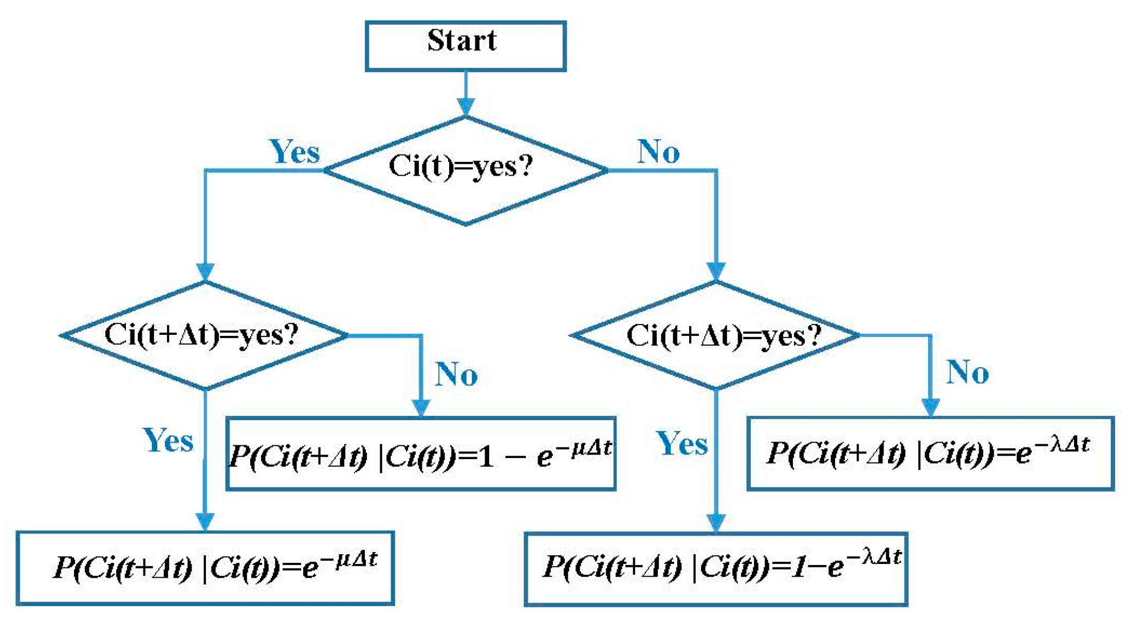
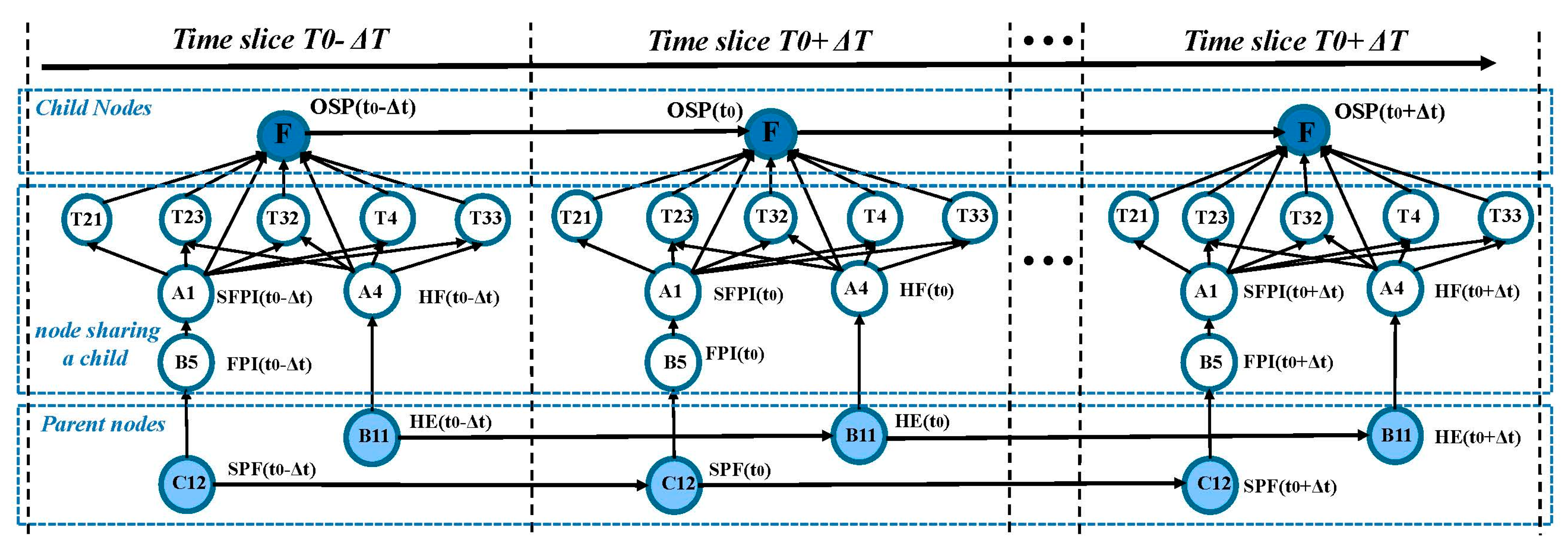
3.4. Determine the Transfer Probability of the Nodes of a Dynamic Bayesian Network

The transfer process in dynamic Bayesian network nodes follows the Markov process. Hence, some nodes in the dynamic Bayesian network have multiple states, and the probability of these nodes being in a certain state shifts as time passes.

(i)

Transfer the probability of sump pump failure

Suppose the failure rate of the sump pump is λ and the repair rate is μ. Then, there are two states: yes and no, where yes means the equipment is faulty; no means the equipment is functional. Assuming that the current moment is t and the next moment is t + Δt, a Markov transfer model for the device in two states is established, as shown in Figure 5. Based on the state transfer model, the equipment takes repair measures and the node state transfer probability as described in Equations (13)–(16) [27].

$$P(C_{i,t+1}=yes|C_{i,t}=yes)=e^{-\mu \Delta t}$$

(13)

$$P(C_{i,t+1}=no|C_{i,t}=yes)=1-e^{-\mu \Delta t}$$

(14)

$$P(C_{i,t+1}=yes|C_{i,t}=no)=1-e^{-\lambda \Delta t}$$

(15)

$$P(C_{i,t+1}=no|C_{i,t}=no)=e^{-\lambda \Delta t}$$

(16)

(ii)

Human error transfer probability

In construction operations, each operation has two states of success and failure. Human error is a random event, assuming that the number of human errors during the operation is a random independent variable and that the human error random variable is a counting process and satisfies a Poisson distribution. Assume that the average value of the number of human errors per unit of time is λ; in this case, the human error state is only related to the previous moment state and not to the past moment state. Hence, the human error state is consistent with the chi-square Markov transfer chain [23]. Equations (15)–(18) calculate the node state transfer probability.

$$P(C_{i,t+1}=yes|C_{i,t}=no)=\lambda e^{-\lambda }$$

(17)

$$P(C_{i,t+1}=no|C_{i,t}=no)=1-\lambda e^{-\lambda }$$

(18)

$$P(C_{i,t+1}=no|C_{i,t}=yes)=e^{-\lambda }$$

(19)

$$P(C_{i,t+1}=yes|C_{i,t}=yes)=1-e^{-\lambda }$$

(20)

3.5. Dynamic Analysis of Coupled Risk Dynamics Based on Dynamic Bayesian Networks

The dynamic analysis of coupled risks based on dynamic Bayesian networks includes three aspects before, during, and after an accident.

1.

A priori analysis (causal inference):

A priori analysis is based on the combination of risk factors in different states to infer the final result of the overall project risk. A priori analysis predicts the probability distribution of the general risk event F under the combination of each risk factor C₁, C₂, … C_i, …, C_n. The prior probability of each risk factor is entered into the network model, and the probability distribution of F is shown in Equation (21).

$$P(F=Stat{e}_f)={\displaystyle \sum _1^{m^n}P(f=Stat{e}_f|C_1=c_j,C_2=c_j,\dots C_n=c_j)\times }P(C_1=c_j,C_2=c_j,\dots C_n=c_j)$$

(21)

where n is the number of nodes; c_j is the jth state of the root node (j = 1,2,…,m); State_f is the fth state of the leaf node (f = 1,2,…,F); $P(f=Stat{e}_f|C_1=c_j,C_2=c_j,\dots C_n=c_j)$ is the conditional probability distribution when f = State_f; and $P(C_1=c_j,C_2=c_j,\dots C_n=c_j)$ is the joint probability distribution.

2.

Sensitivity analysis

Sensitivity analysis can determine the importance of risk influencing factors or hazardous events, identify important targets to focus on safety design or risk monitoring, and help managers make the right decisions for risk management [28,29].

Information entropy is a statistic that describes the dispersion of random variables; the greater the information entropy, the greater the uncertainty. The information entropy of the construction accidents probability in DFPs adjacent to existing underpass tunnels is calculated using Equation (22). Mutual information indicates the amount of information shared between two or more variables. Moreover, the larger the mutual information, the stronger the correlation between the variables. The mutual information also enables finding the key risk factors that greatly impact the overall risk. For example, the mutual information between variables F and C can be calculated using Equation (23).

$$H(F)=-{\displaystyle \sum _{f}P(f)}\log P(f)$$

(22)

$$H(C:F)={\displaystyle \sum _{f\in F}{\displaystyle \sum _{c\in C}p(c,f)}}{\log }_2\left(\frac{p(c,f)}{p(c)p(f)}\right)$$

(23)

where $p(c,f)$ is the joint probability distribution of C and F, and $p(c)$ and $p(f)$ are the marginal distribution probabilities of C and F, respectively.

3.

A posteriori analysis (causative analysis):

The posterior analysis aims to obtain the posterior probability distribution of each risk factor at the time of the accident to detect the suspected cause quickly. Based on the model structure and parameters, the most likely combination of causes in the event of a construction accident in a DFP adjacent to existing underpass tunnels (i.e., the causes derived from the conclusions and assisting engineers in real-time accident diagnosis) is determined. According to Section 2.2.1, the calculation equation is as follows:

$$P(C_i=c_j|F=Stat{e}_f)=\frac{P(C_i=c_j)P(F=Stat{e}_f|C_i=c_j)}{P(F=Stat{e}_f)}$$

(24)

where $P(C_i=c_j|F=Stat{e}_f)$ is the posterior probability distribution of the ith risk factor $C_i$ when $F=Stat{e}_f$.

3.6. Model Validation

The constructed dynamic Bayesian network model for analyzing DFP projects adjacent to existing underpass tunnels must be subjected to a critical model validation process to ensure the reasonableness and accuracy of the analysis results. The model must be partially validated and must satisfy the following three axioms [30]:

Axiom 1: A slight increase (decrease) in the prior probability of each parent node leads to a relative increase (decrease) in the posterior probability of the child nodes.

Axiom 2: If a parent node changes the subjective probability distribution, the magnitude of its effect on the child node values should remain the same.

Axiom 3: The total effect magnitude of the combination of probability changes from x nodes on the values should always be larger than the effect from x–y ($y\in x$) nodes.

4. Case Study

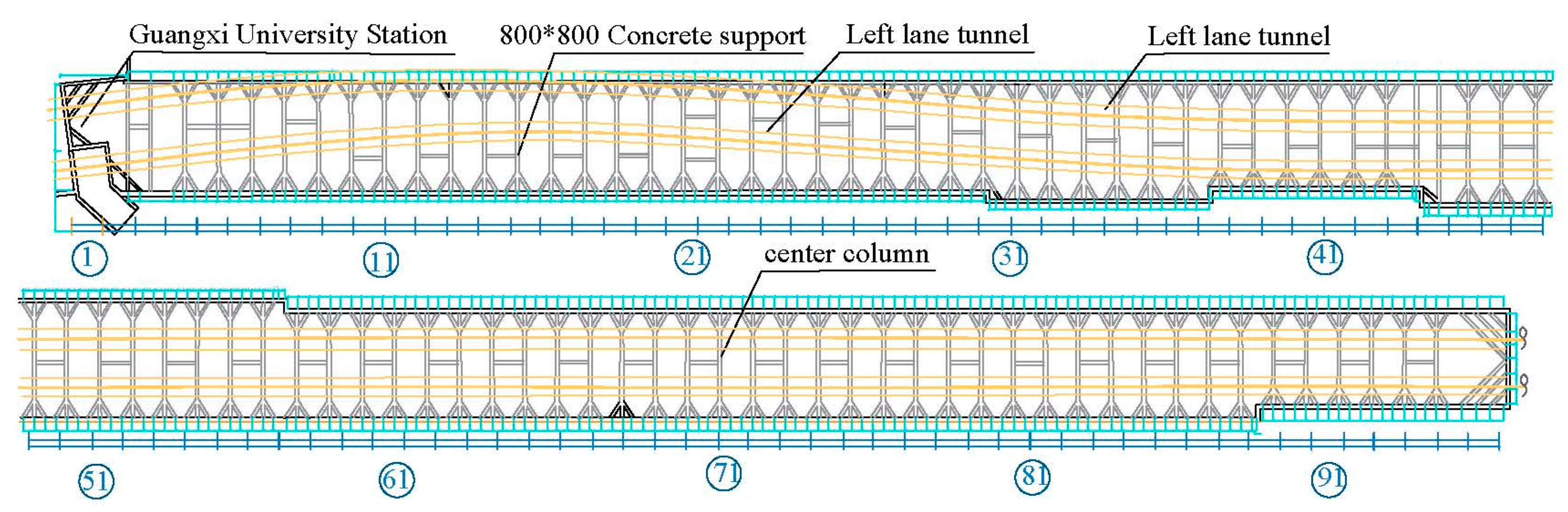
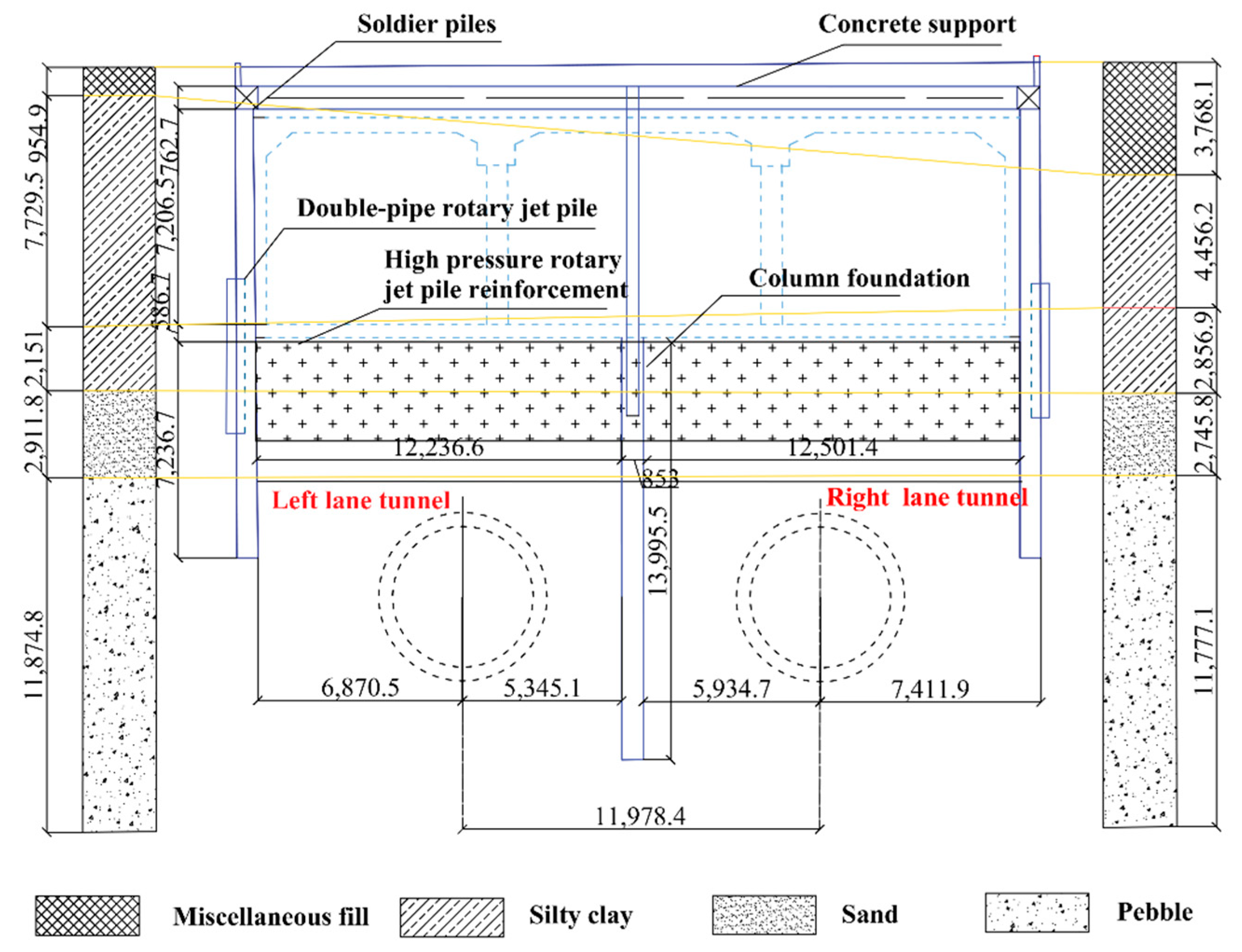
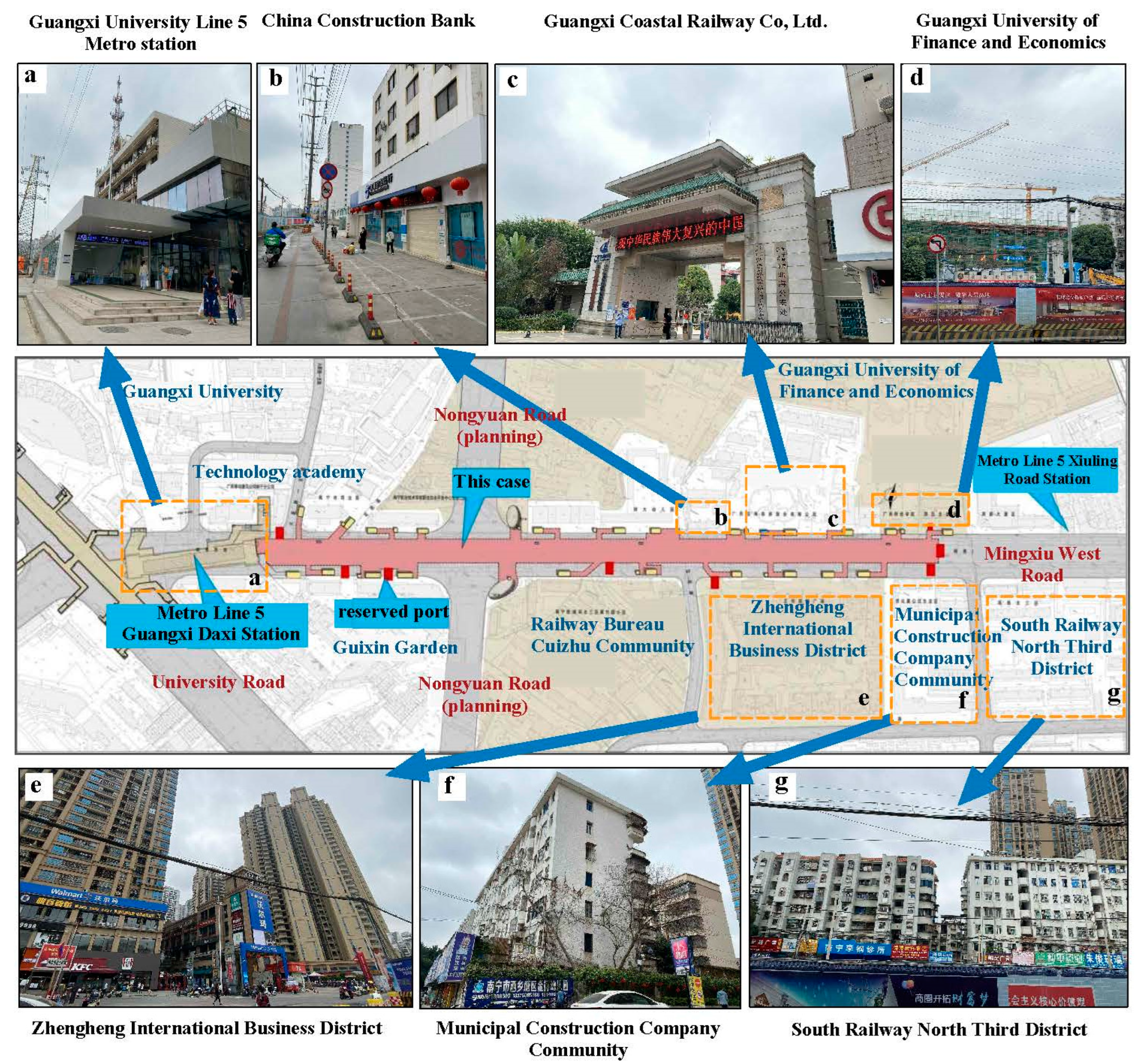
4.1. Project Overview

This study took the underground space utilization project of Nanning rail transit Line 5 (Guangxi University station to Guangxi University of Finance and Economics) as the case study for validating the developed risk coupling analysis method based on the dynamic Bayesian network and N–K model. In order to establish a dynamic Bayesian network, a large dataset was collected during the excavation of the DFP adjacent to the existing underpass tunnel. The total length of the case’s main structure is 811.2 m, the standard width of the main pit is 28.8 m, and the pit’s depth is 8.6–10.5 m. The main pit enclosure structure of the project adopted the support form of ϕ800 bored piles with internal support, and ϕ600 double pipe rotary piles were used to prevent water between the piles. The foundation pit support system adopted two supports, as shown in Figure 6. The surrounding facilities of the project are extremely complicated, and the project is located above the interval between Guangxi University Station and Xiuling Road Station of Line 5. The clear vertical distance is 5–8.7 m. The soil at the pit bottom is reinforced before excavation to reduce the pit uplift and tunnel uplift and strengthen the monitoring in the pit and tunnel. Various monitoring items and the distribution of monitoring points are shown in Figure 7. The geological and enclosure structure profile is shown in Figure 8. Notably, pore water represents the majority of the groundwater in the site, which is stored in the compressive conglomerate layer. In addition, buildings such as Nanning Vocational and Technical College, Guangxi Finance and Economics College Teaching Building, and Construction Bank Mingxiu West Road Branch are adjacent to the project pit. The overview of the surrounding buildings and environment is shown in Figure 9.

The Nanning Line 5 Guangxi University Station–Xiuling Road Station interval of tunnel line is laid along Mingxiu Road, located directly below the underground space utilization project. The length of the left line of the interval is 1263.597 m, and the length of the right line is 1261.266 m. The total length is 2524.863 m. This interval tunnel burial depth is ~9.71–18.72 m, mainly through the round gravel layer, pebble layer, and powder-fine sand layer. The project shield interval tunnel inner diameter is 5400 mm, the lining thickness is 300 mm, the strength grade is C50, and the seepage resistance grade is P12. The shield tunnel cross-section and its detection point layout are shown in Figure 10.

4.2. Monitoring Data Collection and Processing

The data relating to risk factors in this study were obtained from the excavation process of the project, the DFP itself, the tunnel, and the surrounding environmental system deformation monitoring including settlement class, lateral shift class, stress class, and other monitoring data. In this study, 143 sets of sample data containing the risk factors and pit safety status were collected, with 102 sets of high safety, 36 sets of medium safety, and five sets of low safety. Among these data, 123 sets of data were used to train the Bayesian network risk-coupled dynamic model, and the other 20 sets were used to test the model.

Table 1. Original monitoring data.

	Risk Factors							Overall Project Risk Indicators
No.	Heaped Load q (KPa)	Storm Water Volume Q (mm)	Soil Exposure Time T (h)	…	Unit Weight of Soil γ (KN/m3)	The Angle of Internal Friction φ (°)	Cohesive Forces of Soil c (KPa)	Surrounding Surface Sedimentation (mm)	Bottom Heave (mm)	…	Lateral Displacement of Enclosure (mm)
1	4.58	12.4	9	…	18.7	7	13	−3.8724	5.4341	…	−4.5328
2	4.49	64.2	8	…	18.7	7	13	−3.3455	11.6254	…	−5.3243
3	4.98	0.0	7	…	19.6	12	50	−4.5126	9.5108	…	−6.5427
4	5.34	5.8	12	…	19.6	12	50	−2.1458	8.1652	…	−4.2258
5	3.98	0.0	10	…	19.6	12	50	−2.5219	12.8014	…	−5.1078
6	4.17	0.0	8	…	19.2	11	30	−2.9757	11.5201	…	−4.0549
7	4.95	0.0	9	…	19.6	12	50	−4.5542	7.0734	…	−5.5245
8	6.24	0.0	10	…	19.6	12	50	−9.8245	15.9219	…	−5.4378
9	5.83	205.9	13	…	19.2	11	30	−8.4597	18.4524	…	−4.3218
10	7.84	72.5	9	…	19.2	11	3	−11.3248	19.5203	…	−2.4245
…	…	…	…	…	…	…	…	…	…	…	…
136	5.39	9.0	15	…	18.1	3	5	−5.5256	10.3251	…	−3.4324
137	9.51	0.0	18	…	18.1	3	5	−3.4457	11.4983	…	−4.5267
138	8.37	14.3	14	…	22.0	33	0	−9.2864	9.7247	…	5.6271
139	12.84	11.8	15	…	22.0	33	0	−2.7458	14.6214	…	3.8245
140	11.92	0.0	10	…	19.2	11	30	−11.8124	8.6328	…	9.7794
141	16.07	0.0	8	…	19.6	12	50	−14.1579	12.8047	…	−3.5124
142	8.64	8.5	19	…	19.6	12	50	−4.2781	12.4125	…	−2.4469
143	9.75	0.0	14	…	19.6	12	50	−7.6413	13.2934	…	9.7728

shows the sample data used for model training.

The collected data related to the risk factors of the DFPs adjacent to the existing underpass tunnels were processed for risk classification. Moreover, these data are either numerical or textual. Hence, they were discretized according to the Code for monitoring measurement of urban rail transit engineering (GB 50911-2013), as shown in

Table 2. Discrete state description and a priori probability of influence factors of DFPs in adjacent existing underpass tunnels.

Risk Events	Levels	Description	Prior p	Risk Events	Levels	Description	Prior p
C1 Insufficient soil strength (ISS)	Yes	Soil reinforced	0.015	C18 Excavation is too fast (ETF)	Low	L > 0.7 H	0.035
	No	Soil reinforcement	0.985		Medium	0.3 H < L ≤ 0.7 H	0.353
C2 Insufficient support resistance (ISR)	Yes	Whether the resistance reaches the design value	0.026		High	L ≤ 0.3H	0.612
	No		0.974	C19 Mechanical operation regularity (MOR)	Low	The degree of regulation of operation	0.246
C3 Support load overload (SLO)	Yes	Whether the actual axial force exceeds the design value	0.124		Medium		0.452
	No		0.876		High		0.302
C4 Heaped load (HL)	Low	q > 20 KPa	0.041	C20 unit weight of soil (UWS)	Low	γ > 19%	0.098
	Medium	15 KPa < q ≤ 20 KPa	0.185		Medium	17% < γ ≤ 19%	0.548
	High	q ≤ 15 KPa	0.774		High	γ ≤ 17%	0.354
C5 Release slope too steep (RSS)	Yes	The sloping coefficient k > 0.7	0.418	C21 The angle of internal friction of soil (AIFS)	Low	ψ ≤ 9	0.121
	No	The sloping coefficient k ≤ 0.7	0.582		Medium	9 < ψ ≤ 18	0.374
C6 Excessive amount of water in the storm (EWS)	Yes	Q > 200 mm	0.359		High	ψ > 18	0.505
	No	Q < 200 mm	0.641	C22 The cohesive forces of soil (CFS)	Low	c ≤ 10	0.057
C7 Excessive soil exposure time (ESET)	Low	T > 24 h	0.116		Medium	10 < c ≤ 20	0.483
	Medium	18 < T ≤ 24 h	0.587		High	c > 20	0.460
	High	T ≤ 18 h	0.297	B1 bottom heave (BH)	Yes	Whether the bottom is heaving	0.012
					No		0.099
C8 Hole collapse (HC)	Yes	Hole collapse occurs	0.085
	No	No hole collapse	0.915	B2 Support instability (SI)	Yes	Whether the support deformation instability	0.012
C9 Broken Pile (BP)	Yes	Jet grouting pile deformation	0.074		No		0.988
	No	No deformation	0.926	B3 Slope slip (SS)	Yes	Whether slope instability occurs	0.243
C10 Depth of retaining structure into soil (DRSS)	Low	W ≤ 0.7 H	0.021		No		0.976
	Medium	0.7 H < W ≤ 0.9 H	0.193	B4 Instability of retaining structure (IRS)	Yes	Whether the retaining structure is destabilized	0.065
	High	W > 0.9 H	0.786		No		0.935
C11 Leakage occurred in the sealing curtain (LOSC)	Yes	Whether the curtain has water seepage	0.184	B5 Foundation pit inrush (FPI)	Yes	Whether a sudden water-inrush accident occurs	0.064
	No		0.816		No		0.936
C12 Sewage pump failure (SPF)	Yes	Whether the sewage pump is faulty	0.076	B6 Differential settlement of tunnel structure (DSTS)	Yes	Whether uneven settlement occurs	0.037
	No		0.924		No		0.964
C13 High groundwater level (HGL)	Low	D > −8 m	0.047	B7 Excessive convergence of tunnel section (ECTS)	Yes	Whether the tunnel section is excessive convergence	0.063
	Medium	−10 m < D ≤ −8 m	0.216		No		0.937
	High	D ≤ −10 m	0.737	B8 Building inclination and damage (BID)	Yes	Whether damage occurs to the surrounding buildings	0.068
C14 Uneven excavation and unloading (UEU)	Yes	Does the excavation meet the specifications	0.308		No		0.932
	No		0.692	B9 Uneven ground settlement (UGS)	Yes	Whether the surface is unevenly settled	0.015
C15 Uneven soil layer underneath (USLU)	Yes	Uneven stratigraphic conditions	0.274		No		00985
	No		0.726	B10 Failure to follow operating procedures (FOP)	Yes	Whether there are irregular operations	0.075
C16 Excess Excavation (EE)	Low	Over-excavation ≤ 10%	0.241		No		0.925
	Medium	10% < Over-excavation ≤ 30%	0.315	B11 Human error (HE)	Yes	Whether fatigue and distraction	0.043
	High	Over-excavation > 30%	0.444		No		0.957
C17 Presence of weak interlayer (PWI)	Low	P > 30%	0.292	A1 Stability of foundation pit itself (SFPI)	Low	Comprehensive evaluation by experts	0.038
	Medium	10 < P ≤ 30%	0.241		Medium		0.310
	High	P ≤ 10%	0.467		High		0.652
A2 Stability of existing tunnel (SET)	Low	Comprehensive evaluation by experts	0.117	A3 Stability of surrounding environment (SSE)	Low	Comprehensive evaluation by experts	0.056
	Medium		0.284		Medium		0.226
	High		0.600		High		0.718
A4 Human factors (HF)	Low	Comprehensive evaluation by experts	0.265	F Overall safety of the project (OSP)	Low	Comprehensive evaluation by experts	0.105
	Medium		0.250		Medium		0.235
	High		0.484		High		0.659

, wherein low, medium, and high represent the safety degree. The lower the safety level, the more unsafe and dangerous the risk factor.

4.3. Association Rule Mining

The number of association rules obtained gradually decreases as the threshold values of support and lift become larger. Although this part of the association rules obtained is more effective, at the same time, more useful data may be missed. In contrast, the smaller the thresholds of support and confidence, the larger the number of association rules obtained, but may be interspersed with some worthless data, making it difficult to filter out useful conclusions. This study refers to the relevant research experience of using association rules to solve similar geotechnical engineering problems [3]. According to the statistical data of risks in this case and the actual construction situation, this paper analyzed the number of association rules obtained by different support and promotion degrees, and weighs the influence of two extremes. It was concluded that the association rules obtained when the minimum support degree was 0.4 and the minimum promotion degree was 1.1 could achieve the best effect. Then, the Apriori algorithm was used to analyze the frequent item set of the construction risk of DFP adjacent to the existing underpass tunnel, as shown in

Table 3. Frequent item set of construction risks of DFPs in adjacent existing underpass tunnels.

Two Frequent Item Sets	Support	Three Frequent Item Sets	Support	Four Frequent Item Sets	Support
{SLO-Y, SI-Y}	0.511	{ISR-Y, SLO-Y, SI-Y}	0.452	{SS-Y, HL-M, RSS-Y, SFPI-M}	0.405
{RSS-Y, SS-Y}	0.498	{RSS-Y, EWS-M, SS-Y}	0.471	{HL-M, RSS-Y, SS-Y, EWS-L}	0.409
{UGS-Y, CFS-L}	0.492	{BP-Y, DRSS-L, IRS-Y}	0.422	{SET-M, UEU-Y, USLU-Y, DSTS-M}	0.401
{HF-Y, FOP-Y}	0.507	{DRSS-M, HC-Y, IRS-Y}	0.455	{SSE-M, BID-Y, UGS-Y, UWS-M}	0.411
{BH-Y, ISS-N}	0.514	{UEU-Y, DSTS-Y, EE-Y}	0.436	{SS-Y, SI-Y, BH-Y, SFPI-M}	0.413
{HF-Y, HE-Y}	0.489	{PWI-M, ETF-L, ECTS-Y}	0.408	{IRS-Y, HC-Y, BP-Y, SFPI-Y}	0.414
{IRS-Y, DRSS-L} …	0.496 …	{UWS-M, CFS-M, UGS-Y} …	0.434 …	{FPI-Y, SFPI-M, SPF-Y, HGL-Y} …	0.408 …

.

The association rules of the DFP project adjacent to the existing underpass tunnel mined by the Apriori algorithm analysis are shown in

Table 4. Schematic of the association rules.

Left Side of Association Rules	Right Side of Association Rules	Lift	Support	Confidence
{UEU-Y, DSTS-Y, EE-Y}	{SET-M}	1.3327	0.581	0.983
{PWI-M, ETF-L, ECTS-Y}	{OSP-M, SET-M}	1.3319	0.560	0.982
{SS-Y, HL-M, RSS-Y, SFPI-M}	{OSP-M}	1.3218	0.552	0.982
{IRS-Y, HC-Y, BP-Y, LOSC-Y}	{SFPI-M}	1.3201	0.561	0.966
{PWI-M, ETF-L, ECTS-Y}	{OSP-M, SET-M}	1.3105	0.540	0.931
{HL-M, RSS-Y, SS-Y, EWS-L}	{OSP-M, SFPI-M}	1.3098	0.551	0.932
{DRSS-M, HC-Y, IRS-Y}          …	{SFPI-M} …	1.3051 …	0.511 …	0.879 …

. As mentioned previously, the correlations filtered by the association rules must meet at least the minimum support or lift.

4.4. Risk Coupling of DFP Construction in Adjacent Existing Underpass Tunnels

In this study, 86 risk events from 51 similar engineering projects that the Survey and Design Institute Group Ltd. was involved in over the period from 2015 to 2021 were compiled and counted, as shown in

Table 5. Risk coupling frequency and probability for 86 cases.

Types of Risk Coupling	Involving Risk Factors	Times	Probability
Single-factor risk coupling	Foundation pit	6	P1000 = 0.070
	Existing tunnel	1	P0100 = 0.012
	Surrounding environment	24	P0010 = 0.279
	Human factors	12	P0001 = 0.140
Double-factor risk coupling	Foundation pit–existing tunnel	4	P1100 = 0.047
	Foundation pit–surrounding environment	16	P1010 = 0.186
	Foundation pit–human factors	3	P1001 = 0.035
	Existing tunnel–surrounding environment	2	P0110 = 0.023
	Existing tunnel–human factors	0	P0101 = 0.000
	Surrounding environment–human factors	8	P0011 = 0.093
Multifactor risk coupling	Foundation pit–existing tunnel–surrounding environment	6	P1110 = 0.070
	Foundation pit–existing tunnel–human factors	0	P1101 = 0.000
	Foundation pit–surrounding environment–human factors	2	P1011 = 0.023
	Existing tunnel–surrounding environment–human factors	1	P0111 = 0.012
	Foundation pit–existing tunnel–surrounding environment–human factors	1	P1111 = 0.012

. Moreover, the coupling degree between various risk factors was calculated.

In order to calculate the mutual information T, the probabilities of occurrence of different coupling cases were calculated, and the results are shown in

Table 6. Different situation probability of risk factor coupling for accidents in DFP adjacent to existing underpass tunnels.

P0...	P1...	P.0..	P.1..	P..0.	P..1.	P…0	P…1	P00..	P01..	P10..	P11..	P0.0.	P1.0.	P0.1.	P1.1.
0.558	0.372	0.826	0.174	0.302	0.698	0.686	0.314	0.512	0.047	0.314	0.128	0.151	0.151	0.407	0.291
P0..0	P1..0	P0..1	P1..1	P.00.	P.10.	P.01.	P.11.	P.0.0	P.1.0	P.0.1	P.1.1	P..00	P..10	P..01	P..11
0.314	0.372	0.244	0.070	0.244	0.058	0.581	0.116	0.535	0.105	0.291	0.023	0.128	0.558	0.174	0.140
P000.	P100.	P010.	P001.	P110.	P101.	P011.	P111.	P00.0	P10.0	P01.0	P00.1	P11.0	P10.1	P01.1	P11.1
0.140	0.105	0.012	0.372	0.047	0.209	0.035	0.081	0.279	0.256	0.035	0.233	0.116	0.058	0.012	0.012
P0.00	P1.00	P0.10	P0.01	P1.10	P1.01	P0.11	P1.11	P.000	P.100	P.010	P.001	P.110	P.101	P.011	P.111
0.012	0.116	0.302	0.140	0.256	0.035	0.105	0.035	0.070	0.058	0.465	0.174	0.093	0.000	0.116	0.023

. Additionally, the coupling degree of two-factor and multi-risk coupling were calculated according to Equations (11) and (12), respectively. For two-factor risk coupling and multi-factor risk coupling, the coupling values are as shown in

Table 7. Coupling values of each risk factor for construction accidents in the DFPs of adjacent existing underpass tunnels.

T21	T22	T23	T24	T25	T26	T31	T32	T33	T34	T4
0.183	0.115	0.178	4 × 10−4	2 × 10−4	0.091	0.174	0.238	0.343	0.176	0.463

. Therefore, the coupling values were arranged as follows: T4 > T33 > T32 > T21 > T23 > T34 > T31 > T22 > T26 > T24 > T25. The results show that multi-factor coupling usually has a higher coupling degree than two-factor coupling, but there are also cases where the multi-factor coupling degree is lower than the two-factor coupling degree such as T23 > T34. Moreover, the larger the coupling degree value, the greater the interaction of risk factors; hence great attention must be paid to this point. This study combined the expert recommendations and summaries of historical accidents, attached great significance to coupling cases with a coupling degree greater than or equal to 0.1, and introduced nodes T4, T33, T32, T21, and T23 in the Bayesian network. Therefore, the overall risk is not only influenced by SFPI (A1), SET (A2), SSE (A3), and HF (A4) but is also affected by multi-factor coupling.

4.5. Establishment of Dynamic Bayesian Network for Construction Risk of DFPs Adjacent to Existing Underpass Tunnels

The determination of the Bayesian network structure is mainly based on the correlation between the risk factors in the network. The correlation between the nodes can be initially judged according to the correlation of association rules, as shown in Figure 11. Furthermore, it is necessary to correct the correlation based on the degree of risk coupling obtained from the N–K model. Because the occurrence probability of some risk factors increases with time, some risk factors are set as dynamic nodes, and the dynamic Bayesian network for analyzing the construction risk of the DFP adjacent to the existing underpass tunnel is shown in Figure 12 (the nodes with constant probability have been simplified). However, the probability of sewage pump failure and the probability of human error will change with time, according to the relevant parameters provided by the equipment manufacturer and the statistics of similar engineering accidents, assuming that the failure rate of the sewage pump is 0.156, the repair rate is 1.72 × 10⁻² and the average number of human errors per unit of time is 3.95. In this paper, a dynamic Bayesian network model with 20 time slices was built using Netica software. The time interval between any two slices was taken as 7 days, and the first time slice ranged from 13 December 2021 to 19 December 2021. Based on a large amount of processed settlement and deformation monitoring data of the foundation pits and tunnels, the prior probability distribution of each node was obtained by the parameter learning method.

4.6. Model Validation Stage

In this study, a coupled dynamic Bayesian network was established for the risk of DFPs adjacent to existing underpass tunnels, and 20 additional sets of data collected previously were input into the model. The risk states obtained from the Bayesian inference were compared with the actual risk states to validate the model, and the validation results are shown in

Table 8. Model validation (comparison of predicted and actual results).

No.	Test Samples	Safety of DFPs Adjacent to Existing Underpass Tunnels			Expectation	Actuality
		High	Medium	Low
1	C1 = No; C3 = Yes; C13 = Low; C14 = No; B5 = Yes	64.8%	24.8%	10.5%	High	High
2	A1 = Medium; A2 = Low; B7 = No; B7, B11 = Yes	43.3%	43.6%	13.1%	Medium	Medium
3	A2 = Medium; B5, C11, C3 = Yes; B6 = No; C18 = High	60.5%	28.6%	10.9%	High	High
4	C1, C3 = Yes; B2, C12 = No; C13, C22 = High	67.0%	23.0%	10.0%	High	High
5	A4, A1 = Low, B6, B7, B8, B9 = Yes	42.3%	42.4%	15.2%	Medium	High
6	B5 = No; C2 = Yes; C18 = High; A1 = Medium	49.8%	38.0%	12.2%	High	High
7	A4 = Medium, B2, B7 = Yes, B5, C2 = No, C20 = Low	62.0	26.9%	11.1%	High	High
…	…	…	…	…	…	…
19	B8, B6, C11, C12 = No; B2 = Yes; C17 = High	64.3%	25.1%	10.6%	High	High
20	B2, B3, B8, B9,C11, C12 = No; C13, C21, C16 = High	59.6%	29%	11.4%	High	High

. Of the 20 test samples, only the third group’s results did not agree with the actual measurements, which means that the model’s accuracy was 95%. In addition, the proposed coupled dynamic Bayesian network model was partially validated for the risk of DFPs adjacent to existing underpass tunnels. For example, when the probability of the low safety of foundation pits, existing tunnels, surrounding environment, and human factors is set to 100%, the probability of low safety of the overall risk increases from 9.96% to 13.1%, 14.0%, 14.7%, and 15.6%, respectively. In contrast, when the high probability of the safety degree for these parent nodes is set to 100%, the low safety degree probability of the overall risk decreases from 9.96% to 9.09%, 8.73%, 8.42%, and 7.83%, confirming the three axioms. In summary, the accuracy of the constructed coupled dynamic Bayesian network model for the risk of DFPs adjacent to existing underpass tunnels was verified, and the model can be used for risk assessment in similar projects.

5. Results and Discussion

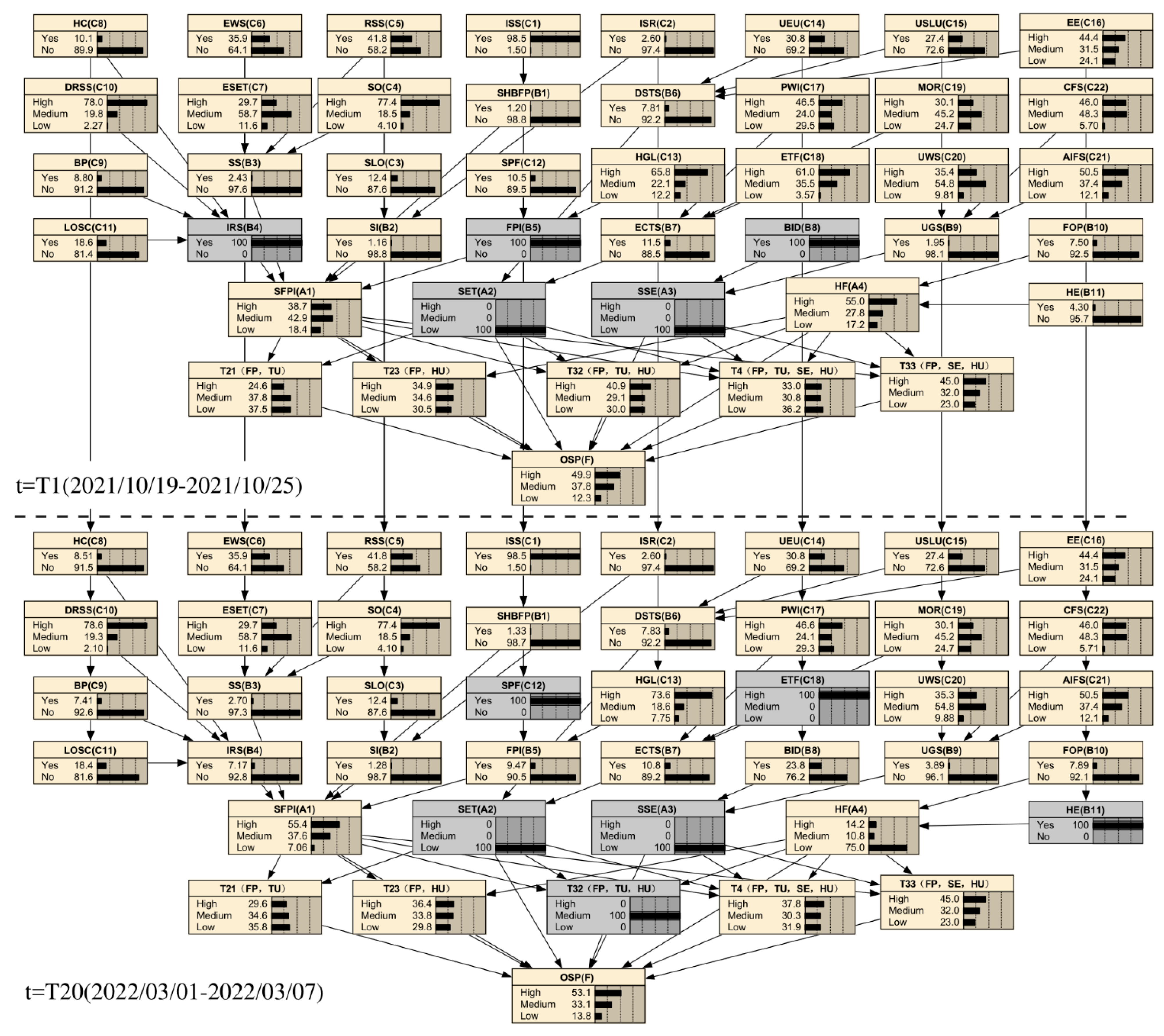
5.1. Risk Prediction Based on Dynamic Bayesian Networks for Foundation Pits Adjacent to Existing Underpass Tunnels

The probabilities were updated by inputting the new state information of the root node, and the probabilities were propagated along the dynamic Bayesian network. Then, the risk probability of the foundation pit project was automatically calculated for different time slices under different conditions. The project manager can accurately predict the risk status of the DFP adjacent to the existing underpass tunnel during each monitoring period.

Figure 13 shows the combination of risk factors for constructing DFPs adjacent to existing underpass tunnels under eight different scenarios. Figure 14 represents the Bayesian network risk prediction process for Scenario 4 at moment T1 and Scenario 5 at moment T20, and Figure 13 depicts the probabilistic prediction results of the DBN model for eight different scenarios and various time premises. The probability that the construction of DFPs adjacent to existing underpass tunnels is at a low safety level under eight different scenarios at the T1 time slice was divided into 9.9%, 10.8%, 11.4%, 12.3%, 13.8%, 15.8%, 15.1%, and 12.2%, and under the T20 time slice, the probabilities were 10.8%, 11.6%, 11.4%, 13.8%, 14.1%, 16.7%, 15.5%, and 12.9%. The findings showed that (I) the prediction results of the construction risk level of DFPs adjacent to existing underpass tunnels vary in different scenarios. When no risk factors occur, the overall safety of the foundation pit is high. When multiple risk factors occur, (I) the probability that the DFP is at a low level of safety will be higher than when no risk factors or only a single factor occurs. (II) The higher the level of risk factors present, the greater the impact on the overall risk (e.g., A-level risk factors are more influential than B-level). (III) Risk factors at the same level also differ in their influence on overall risk, and the results of probabilistic predictions can qualitatively indicate that SFPI (A1) has more effect than SET (A3). In addition, the outcomes of the prediction of risk levels change as time passes. It is worth noting that the risk prediction probabilities in both Scenario 3 and Scenario 5 are not affected by time. This is presumably because the states of some or all of the dynamic nodes in Scenario 3 and Scenario 5 have already been determined. In this scenario, changes in the probabilities of the dynamic nodes do not affect the predicted results of the overall risk level.

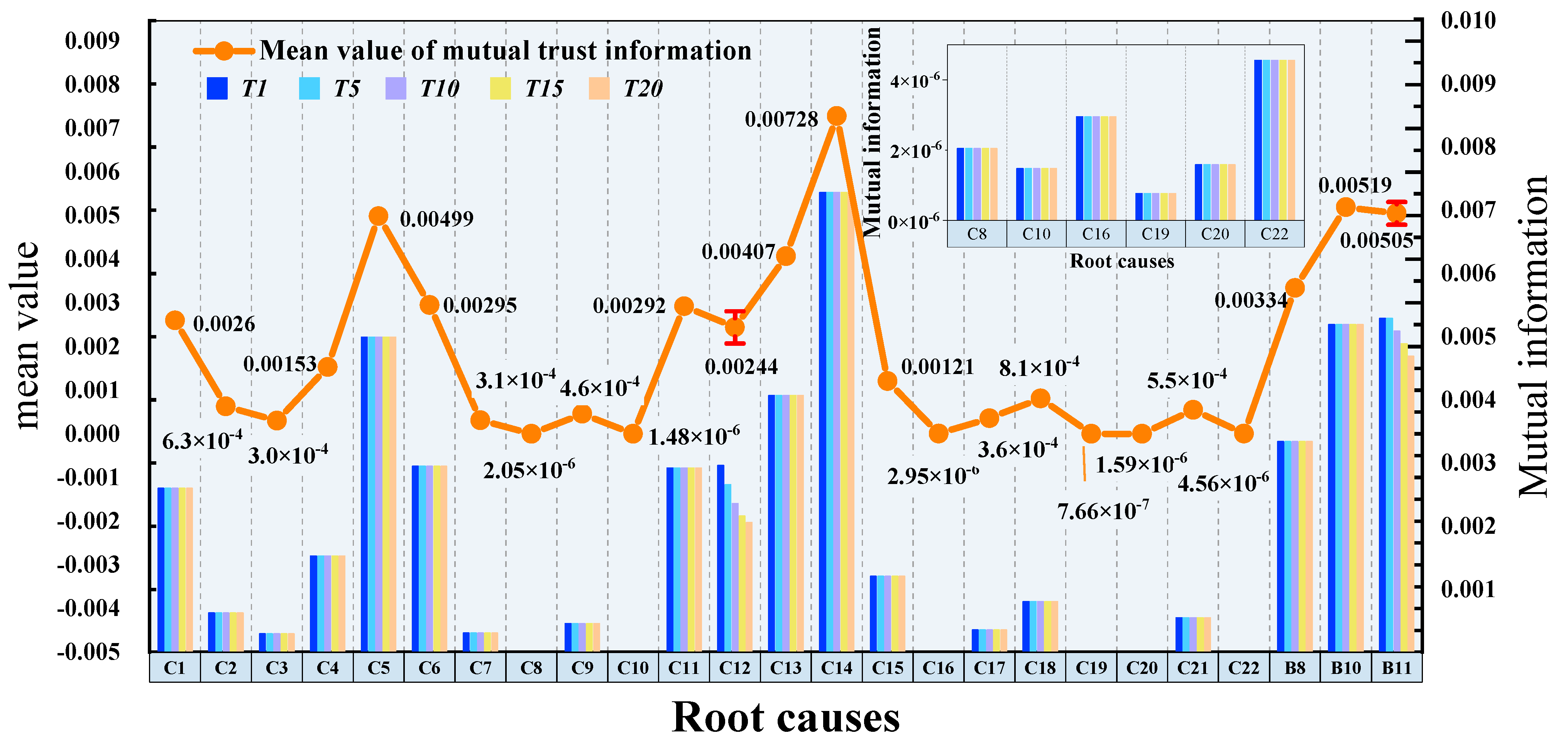
5.2. Mutual Information-Based Sensitivity Analysis

To further determine the factors that need to be given attention to in the risk probability prediction model, this paper used Equation (23) to simulate the mutual information of the nodes at T1, T5, T10, T15, and T20 that cause accidents in the construction of the DFP adjacent to existing underpass tunnels. The analysis results are shown in Figure 15. The mutual information values of most risk factor nodes did not change over time. However, the mutual information between SPF (C12) and HE (B11) decreased with time, and the mutual information between LOSC (C11) and EWS (C6) exceeded that of SPF at T2. The mutual information of RSS (C5) and FOP (B10) exceeded that of B11 at T12 and T7, respectively. The sensitivity analysis results of risk factor nodes change over time and show the importance of introducing node dynamics and updating the prior probabilities of nodes. The top ranking of importance of the nodal variables based on the average of mutual information is FOP (B10), HE (B11), RSS (C5), HGL (C13), and UEU (C14).

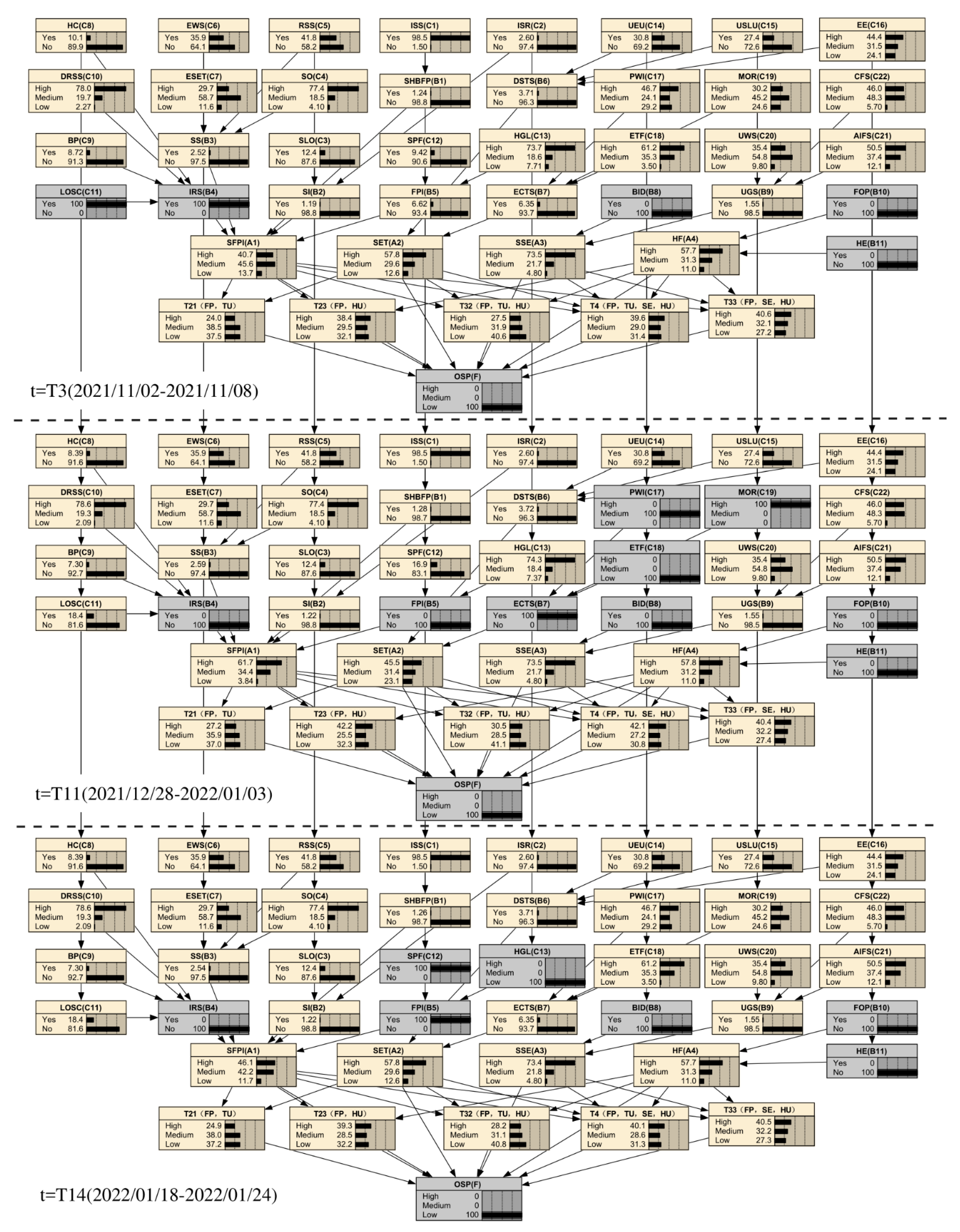
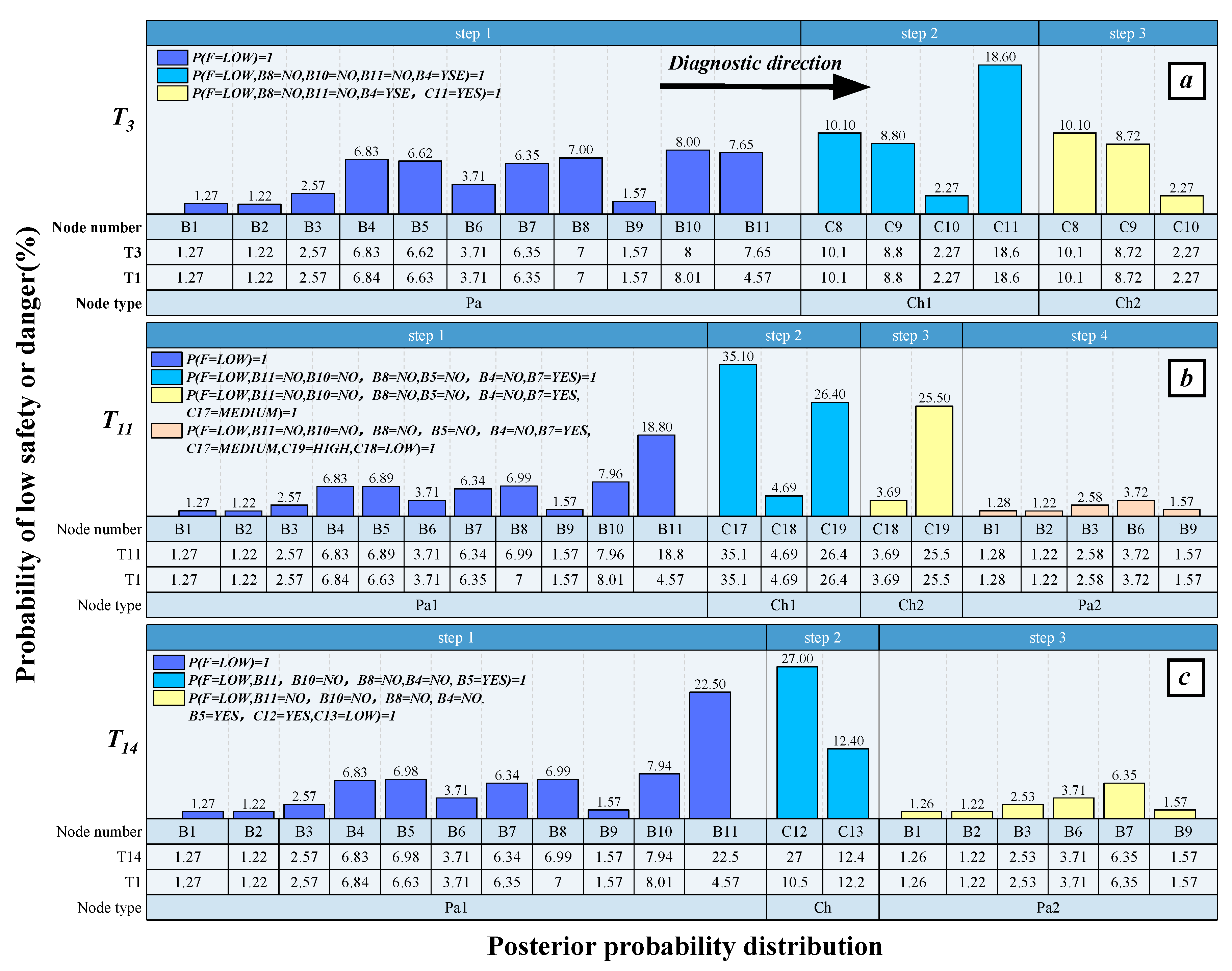
5.3. Practical Application (Backward Inference)

Based on the Bayesian network backward inference, the most likely cause of the accident can be identified as the coupled risk accident in the construction of a DFP in the adjacent existing underpass tunnel (i.e., risk-causing diagnosis can be achieved to help better control the risk and prevent the accident from occurring in future construction). The principle of diagnostic termination is that the risk factor leading to the accident is defined, and the next factor to be examined has not yet occurred. The process of backward inference is shown in Figure 16.

According to the special risk report, on 2 January 2022, the daily settlement rate of rainwater and sewage pipes on the north side of the pit reached 2.3 mm/d, which occurred at time slice T3. In the DBN model of the T3 time slice, the evidence P was set as (F = low) = 1, and the posterior probability distribution of the B level was inferred by the diagnostic function of DBN, as shown in Figure 17a. Based on the posterior probability, there was no FOP (P (B10 = Yes) = 8.00%), HE (P (B11 = Yes) = 7.65%), BID (P (B8 = Yes) = 7.00%) at the accident site. It was not until IRS (P (B4= Yes) = 6.83%) was discovered that the horizontal displacement of the top of the rotary spray pile on the north side of the 64th axis was 37.6 mm in a low safety state. The reverse diagnosis was performed for the C-level risk factors under IRS by setting the evidence P (F = Low, B9 = No, B10 = No, B11 = No, B4 = Yes) = 1, as indicated in Figure 17a. The first risk factor that should be concerned is the occurrence of LOSC (P (C11 = Low) = 18.6%), and the site investigation found a large area of dip on the north side of the 63–68th axis. Construction workers have used high-pressure grouting to form the leaf vein-like structure of cement to seal the gaps in the soil. Figure 18a shows the scene when the danger occurs and demonstrates that there are still many water seepage traces on the concrete of the spray anchor. The spray anchor lag, the continuous seepage of the upper layer of stagnant water affect the water stopping effect of the spray anchor. Let P (C11 = low) = 1, no HC (P (C8 = Low) = 10.1%) was found.

On 21 February 2022 (T11), the 83–84th axis support axial force reached 151.7 kN, more than 70% of the design value. Set evidence P (T = severe) = 1, no risk factors B11, B10, B9, FPI (B5), IRS (B4) occurred until the presence of ECTS (P (B7 = YES) = 6.34%) in the site. Set evidence P (F = Low, B9 = No, B10 = No, B11 = No, B4 = No, B5 = No, B7 = Yes) = 1, as shown in Figure 17b. There were no large weak interlayers in the accident site (P (C17 = Low) = 35.1%) and no irregularity in the operation of machinery (P (C19 = Low) = 26.4%). However, the excavation speed of the pit was too fast (P (C18 =Yes) = 4.69%). At this point, the construction team immediately stopped construction and adjusted the excavation plan. It is worth mentioning that at this point, the tunnel lateral was located within a reasonable range. Setting evidence P (C18 = Low, C19 = High) = 1, no DSTS (B6) was noticed to occur during the subsequent inspections.

On 14 March 2022 (T14), the uplift of the center column at the bottom of the 94th axis of the foundation pit reached 2.14 mm. Based on the previous evaluation logic, the dewatering well between the 92nd and 94th axis had a sudden surge (P (B5 = YES) = 6.98%). As shown in Figure 17c, during the inspection, two risk factors (SPF (C12) and HGL (C13)) occurred in the C-level under FPI (B5). The construction team filled in the small diameter stones at the time of the hazard and filled in the dry material concrete and micro expansion concrete. Figure 18b shows the scene at the time of the dangerous situation. It can be seen that there was a large amount of undrained sewage at the bottom of the pit. It is presumed that the accident occurred as a result of the increased rainfall at that time, coupled with the rupture of the sewage pipe near the pit, which led to the failure of the drainage well and sewage pump due to overloading. In summary, this dynamic Bayesian network model for risk diagnosis can minimize the scope of finding risks and improve the efficiency of handling risky accidents.

6. Conclusions

This study proposed a probabilistic prediction model for the construction risk of DFPs adjacent to existing underpass tunnels using the N–K model and dynamic Bayesian network. The Nanning underground comprehensive utilization project was taken as an example. The risk inference analysis of the DFP construction adjacent to the existing underpass tunnel was conducted from three aspects: probability prediction, sensitivity analysis, and risk diagnosis, which verified the reasonableness and superiority of the model. The following conclusions were drawn:

(1) Using the N–K model, this study quantified the coupling values of various risk factors in the construction accident of DFP of adjacent existing underpass tunnels in different ways: T4 > T33 > T32 > T21 > T23 > T34 > T31 > T22 > T26 > T24 > T25. The results indicated that the more risk factors involved in the coupling, the greater the coupling value. However, a phenomenon where the double factor coupling value is greater than the multi-factor coupling value also appeared, which need to be paid attention to. This study optimized the dynamic Bayesian network model according to the order of the coupling values of risk factors.

(2) Based on the construction data of the DFP project adjacent to the existing underpass tunnel, this study used association rule mining for risk correlation analysis to identify the set of frequent items and the correlation between risks requiring special attention. Based on these correlations and the calculated risk coupling results of the N–K model, a dynamic Bayesian network model was established in this study. It analyzed the node transfer probability of a dynamic Bayesian network using the Markov model. Actual monitoring data were employed to verify the model. The findings showed that the model’s accuracy for risk prediction exceeded 95% and could pass the verification of three axioms, demonstrating the reasonableness of the model.

(3) Through the dynamic Bayesian network coupling risk causal inference, the probability of risk events occurring during the construction of DFP of adjacent existing underpass tunnels can be predicted at various times when the risk factors were in different states. In addition, sensitivity analysis could also be applied to determine the most critical sensitive factor to the risk event among many risk factors at different times. Finally, if an accident occurs, risk diagnosis could be performed according to the model structure and parameters to define the most likely cause combination at a specific time and state.

(4) The results revealed that: (I) there was uneven excavation and unloading (UEU), the slope was too steep (RSS), the groundwater level was too high (HGL), the leakage occurred in the sealing curtain (LOSC), and the building inclination and damage (BID) should be focused on. (II) Risk probability prediction, sensitivity analysis, and risk diagnosis would be affected by dynamic nodes and changed with time, which showed the necessity of introducing dynamic nodes. (III) The risk diagnosis function of the dynamic Bayesian network model for DFP adjacent to an existing underpass tunnel can accurately and quickly identify the accident-causing risk factors, thereby significantly improving the efficacy of handling safety accidents.

References

1. Qian, Q. Present state, problems and development trends of urban underground space in China. Tunn. Undergr. Space Technol. 2016, 55, 280–289. [Google Scholar] [CrossRef]
2. Castaldo, P.; Jalayer, F.; Palazzo, B. Probabilistic assessment of groundwater leakage in diaphragm wall joints for deep excavations. Tunn. Undergr. Space Technol. 2018, 71, 531–543. [Google Scholar] [CrossRef]
3. Zhou, Y.; Li, C.; Ding, L.; Sekula, P.; Love, P.E.; Zhou, C. Combining association rules mining with complex networks to monitor coupled risks. Reliab. Eng. Syst. Saf. 2019, 186, 194–208. [Google Scholar] [CrossRef]
4. Wei, M.; Meng, W.; Dai, F.; Wu, W. Application of machine learning to prediction of rate-dependent compressive strength of rocks. J. Rock Mech. Geotech. Eng. 2022, 14, 1356–1365. [Google Scholar] [CrossRef]
5. Zhang, Y.; Su, G.; Li, Y.; Wei, M.; Liu, B. Displacement Back-Analysis of Rock Mass Parameters for Underground Caverns Using a Novel Intelligent Optimization Method. Int. J. Geomech. 2020, 20, 04020035. [Google Scholar] [CrossRef]
6. Dong, L. Research on the Safety Risk of Existing Tunnel Adjacent to Deep Excavation. Master’s Thesis, Hunan University, Changsha, China, 2018. [Google Scholar]
7. Nezarat, H.; Sereshki, F.; Ataei, M. Ranking of geological risks in mechanized tunneling by using Fuzzy Analytical Hierarchy Process (FAHP). Tunn. Undergr. Space Technol. 2015, 50, 358–364. [Google Scholar] [CrossRef]
8. Wu, X.; Liu, H.; Zhang, L.; Skibniewski, M.J.; Deng, Q.; Teng, J. A dynamic Bayesian network based approach to safety decision support in tunnel construction. Reliab. Eng. Syst. Saf. 2015, 134, 157–168. [Google Scholar] [CrossRef]
9. Sihombing, F.; Torbol, M. Parallel fault tree analysis for accurate reliability of complex systems. Struct. Saf. 2018, 72, 41–53. [Google Scholar] [CrossRef]
10. Kabir, S. An overview of fault tree analysis and its application in model based dependability analysis. Expert Syst. Appl. 2017, 77, 114–135. [Google Scholar] [CrossRef] [Green Version]
11. Zhang, Y.; Wei, M.; Su, G.; Li, Y.; Zeng, J.; Deng, X. A Novel Intelligent Method for Predicting the Penetration Rate of the Tunnel Boring Machine in Rocks. Math. Probl. Eng. 2020, 2020, 3268694. [Google Scholar] [CrossRef]
12. Ding, L.; Fang, W.; Luo, H.; Love, P.E.D.; Zhong, B.; Ouyang, X. A deep hybrid learning model to detect unsafe behavior: Integrating convolution neural networks and long short-term memory. Autom. Constr. 2018, 86, 118–124. [Google Scholar] [CrossRef]
13. Zhang, L.; Wu, X.; Skibniewski, M.J.; Zhong, J.; Lu, Y. Bayesian-network-based safety risk analysis in construction projects. Reliab. Eng. Syst. Saf. 2014, 131, 29–39. [Google Scholar] [CrossRef]
14. Wang, H.; Yajima, A.; Liang, R.Y.; Castaneda, H. Bayesian Modeling of External Corrosion in Underground Pipelines Based on the Integration of Markov Chain Monte Carlo Techniques and Clustered Inspection Data. Comput.-Aided Civ. Infrastruct. Eng. 2015, 30, 300–316. [Google Scholar] [CrossRef]
15. Yang, K. Multi-Factor Coupling Disaster-Causing Mechanism and Disaster Control Study of City Gas Pipeline Leakage. Ph.D. Thesis, Capital University of Economics and Business, Beijing, China, 2016. [Google Scholar]
16. Qiao, W. Analysis and measurement of multifactor risk in underground coal mine accidents based on coupling theory. Reliab. Eng. Syst. Saf. 2021, 208, 107433. [Google Scholar] [CrossRef]
17. Telikani, A.; Shahbahrami, A. Data sanitization in association rule mining: An analytical review. Expert Syst. Appl. 2018, 96, 406–426. [Google Scholar] [CrossRef]
18. Song, K.; Lee, K. Predictability-based collective class association rule mining. Expert Syst. Appl. 2017, 79, 1–7. [Google Scholar] [CrossRef]
19. Luna, J.M.; Cano, A.; Sakalauskas, V.; Ventura, S. Discovering useful useful patterns from multiple instance data. Inf. Sci. 2016, 357, 23–38. [Google Scholar] [CrossRef]
20. Sowan, B.; Dahal, K.; Hossain, M.A.; Zhang, L.; Spencer, L. Fuzzy association rule mining approaches for enhancing prediction performance. Expert Syst. Appl. 2013, 40, 6928–6937. [Google Scholar] [CrossRef]
21. Li, N.; Zeng, L.; He, Q.; Shi, Z. Parallel implementation of apriori algorithm based on mapreduce. In Proceedings of the 2012 13th ACIS International Conference on Software Engineering, Artificial Intelligence, Networking and Parallel/Distributed Computing: IEEE, Kyoto, Japan, 8–10 August 2012; pp. 236–241. [Google Scholar]
22. Pearl, J. Fusion, propagation, and structuring in belief networks. Artif. Intell. 1986, 29, 241–288. [Google Scholar] [CrossRef] [Green Version]
23. Liu, S. A Study on Oil Company Risk of ProductionSafety Based on Employee Behavior Reliability. Ph.D. Thesis, Southwest Petroleum University, Chengdu, China, 2014. [Google Scholar]
24. Kauffman, S.A.; Weinberger, E.D. The NK model of rugged fitness landscapes and its application to maturation of the immune response. J. Theor. Biol. 1989, 141, 211–245. [Google Scholar] [CrossRef]
25. Kauffman, S.A. The Origins of Order: Self-Organization and Selection in Evolution; Oxford University Press: New York, NY, USA, 1993. [Google Scholar]
26. Ganco, M. NK model as a representation of innovative search. Res. Policy 2017, 46, 1783–1800. [Google Scholar] [CrossRef]
27. Kohda, T.; Cui, W. Risk-based reconfiguration of safety monitoring system using dynamic Bayesian network. Reliab. Eng. Syst. Saf. 2007, 92, 1716–1723. [Google Scholar] [CrossRef]
28. Zhang, L.; Wu, X.; Ding, L.; Skibniewski, M.J.; Yan, Y. Decision support analysis for safety control in complex project environments based on Bayesian Networks. Expert Syst. Appl. 2013, 40, 4273–4282. [Google Scholar] [CrossRef]
29. Lee, E.; Park, Y.; Shin, J.G. Large engineering project risk management using a Bayesian belief network. Expert Syst. Appl. 2009, 36, 5880–5887. [Google Scholar] [CrossRef]
30. Jones, B.; Jenkinson, I.; Yang, Z.; Wang, J. The use of Bayesian network modelling for maintenance planning in a manufacturing industry. Reliab. Eng. Syst. Saf. 2010, 95, 267–277. [Google Scholar] [CrossRef]
Figure 1. Steps for association rule mining by the Apriori algorithm.
Applsci 12 10467 g001
Figure 2. Framework of the dynamic and quantitative risk assessment based on the N–K model, ARM, and DBNs.
Applsci 12 10467 g002
Figure 3. Construction accident risk coupling mechanism of DFP adjacent to the existing underpass tunnel.
Applsci 12 10467 g003
Figure 4. Types of risk coupling for accidents in deep foundation projects adjacent to existing underpass tunnels.
Applsci 12 10467 g004
Figure 5. State transition diagram of two-state factors of sewage pump equipment.
Applsci 12 10467 g005
Figure 6. Supporting structure of DFP adjacent to the existing tunnel.
Applsci 12 10467 g006
Figure 7. The layout of monitoring points for the comprehensive underground utilization project of Guangxi University of Finance and Economics.
Applsci 12 10467 g007
Figure 8. Geological section of the envelop enclosure of the comprehensive underground utilization project of Guangxi University of Finance and Economics.
Applsci 12 10467 g008
Figure 9. The surrounding buildings and environment of the underground project of Guangxi University of Finance and Economics.
Applsci 12 10467 g009
Figure 10. Layout of the monitoring points of the existing tunnel.
Applsci 12 10467 g010
Figure 11. Risk factors for the construction of DFPs adjacent to existing underpass tunnels.
Applsci 12 10467 g011
Figure 12. Simplified DBN structure for deep foundation construction in adjacent existing underpass tunnels.
Applsci 12 10467 g012
Figure 13. Percentage values for the safety of construction of DFPs adjacent to existing underpass tunnels in eight scenarios.
Applsci 12 10467 g013
Figure 14. Two scenarios of dynamic Bayesian network modeling for forward inference (T1 and T20).
Applsci 12 10467 g014
Figure 15. Mutual information of root nodes (risk factors).
Applsci 12 10467 g015
Figure 16. Three scenarios of backward inference.
Applsci 12 10467 g016
Figure 17. The posterior probability distributions of the time slices of T3, T11 and T14, as (a), (b) and (c), respectively.
Applsci 12 10467 g017
Figure 18. (a) Leakage of water stop curtain on the north side of the 63–68th axis. (b) Water accumulation due to sudden surge of dewatering well.
Applsci 12 10467 g018