Effect of Secondary Combustion on Thrust Regulation of Gas Generator Cycle Rocket Engine

Abstract

Thrust regulation is applied to maintain the performance of the liquid propellant rocket engine. The thrust level of a rocket engine can be readily controlled by adjusting the number of propellants introduced into the combustion chamber. In this study, a gas generator design is proposed in which thrust regulation is maintained by performing secondary combustion in the divergent section of the nozzle of a gas generator. Tangential and normal injection techniques have also been studied for better combustion analyses. A normal injection technique is used for the experiment and CFD results are validated with the experimental data. Chemical equilibrium analyses are also performed by minimizing Gibbs free energy with the steepest descent method augmented by the Nelder–Mead algorithm. These equilibrium calculations give the combustion species as obtained through the CFD results. Performance evaluation of the rocket engine, with and without secondary combustion in the gas generator, led to an increase of 42% thrust and 46.15% of specific impulse with secondary combustion in the gas generator.

1. Introduction

Thrust regulation in liquid propelled rocket engines (LPRE) is applied to control the mass flow rate to the gas generator (GG) to keep the turbine power at the level necessary to achieve the required thrust chamber pressure. It is carried out by using thrust regulators and secondary combustion in the GG. Thrust regulation through afterburning inside the engine nozzle is of key importance for rocket and jet engines. For space applications, afterburning can be accomplished by injecting propellants (fuel or oxidizer or a combination of both) inside the nozzle divergent section of a rocket engine, which results in much-needed thrust regulation. Though thrust regulation has not been fully applied practically, it has the potential to provide several benefits to expendable and reusable space launch vehicles (ELVs and RLVs) [1,2].

This concept can be applied to ELVs and RLVs in the form of the thrust augmented nozzle “TAN”. Thrust augmentation can be used to re-energize the jet flow, avoid flow separation inside the nozzle, obtain a higher thrust-to-weight ratio, and keep the nozzle optimized throughout the mission, even in a vacuum. Furthermore, this study can also be applied to thrust vectoring in a launch vehicle, which will not only improve its flight performance but will also permit high-g flight maneuvers at reentries and vertical landings. The future of space exploration looks promising, as government and private businesses plan frequent space flights for Moon and Mars expeditions, for which this study could be a cost-effective solution. [3,4].

In rocket engines, secondary combustion in GG has been under study with solid propellants. The interior ballistic stability and ejection efficiency of a rocket are analyzed by conducting secondary combustion in GG of solid-propellant air-turbo rockets through solid propellants. Three-dimensional planar numerical simulation was performed on the secondary combustion and ring-cavity structures by Xiao Lie; furthermore, the combustion effect on the loads and interior ballistic stabilization during ejection was studied [5,6].

Moving to fuel-rich combustion results in more receptiveness to instability and makes it more difficult to achieve the required exhaust temperature. Two-zone GG with ethanol as a secondary fuel gives a stable performance in terms of exhaust temperature. Fuel and oxidizer mass flow rates of the main chamber are controlled through the varying throat cross-sectional area of the GG nozzle, and thrust vector control is achieved [7,8,9].

Secondary combustion in a hybrid rocket engine minimizes the loss of performance by shifting the oxidizer to fuel ratio. Dongeun modelled secondary combustion with gaseous secondary propellant in CFD and compared its results with the experiment. LPRE lacks research in secondary combustion of GG with gaseous oxygen as a secondary oxidizer, and, hence, thrust regulation of the main engine through turbine power. Thrust regulation is done to maintain the performance of the rocket engine. This paper describes the design of a gas generator which can perform thrust regulation for the main rocket engine designed for a lab testing unit. Thrust regulation is achieved by doing secondary combustion in the divergent section of the GG nozzle. Secondary combustion in GG leads to Mach enhancement; hence, giving more power to the turbine shaft, which results in a pressure rise of the pump and an increase in the propellant mass flow of the main combustion chamber. Hence, the overall thrust increment of the main engine is achieved [10,11,12].

For achieving better thrust regulation, in this research, two secondary injection techniques, normal and tangential, were analyzed through CFD and a better performing technique was selected for the prototype development. The experiment was performed using gaseous oxygen (GOX) as a secondary injection propellant, which was obtained by heating the main oxidizer, liquid oxygen (LOX). A comparison is drawn between the thrust achieved with and without secondary injection in GG, which leads to thrust enhancement of the main engine. Through CFD, combustion species were also obtained after secondary combustion. These results were compared after performing chemical equilibrium analyses on the reactants by minimizing Gibbs energy of the system using steepest descent and Nelder–Mead numerical techniques. These CFD results were validated through in-house codes built in Python by using these numerical techniques.

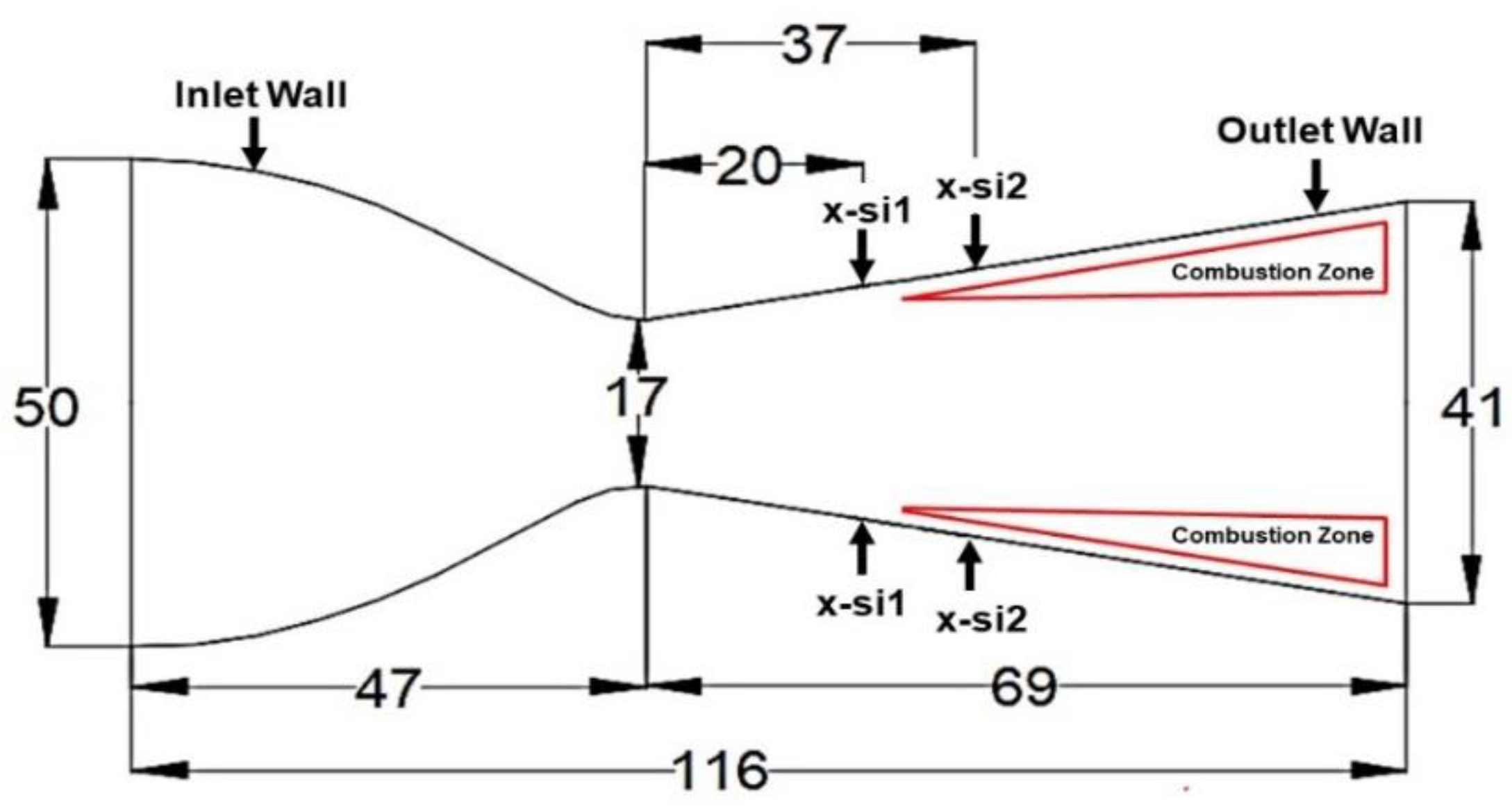
2. Gas Generator Design

Design parameters of the main rocket engine and GG are given in

Table 1. Main rocket engine design parameters.

Design Parameter	Values
Main engine propellants	LOX and RP1
Oxidizer to fuel ratio	2.2
Total flow rate	2.5 kg/s
Chamber pressure	15 bar
Combustion temperature	3090 K
Thrust	5.5 kN

and

Table 2. Gas generator design parameters.

Design Parameter	Values
Gas generator propellants	LOX and RP1
Primary combustion oxidizer to fuel ratio	0.3
Primary injection mass flow rate	0.12 kg/s
Primary chamber pressure	2 bar
Primary combustion temperature	1008 K
Thrust	160 N

, respectively. The GG was designed at 5% of the main engine’s flow. These design parameters were calculated by following Sutton [13]. Figure 1 gives the flow chart of how these design parameters were calculated.

To achieve thrust regulation, the nozzle of GG is kept over-expanded at ϵ = 5.62, so the flow can be detached from the nozzle wall and secondary combustion can be performed in this wake region. This secondary combustion results in a higher exhaust temperature, which lies in the turbine’s working range and high Mach. An increase in the input to the turbine increases the shaft power, resulting in higher rpm and pump pressures. This, as a result, increases the propellant flow to the main chamber and thrust enhancement is achieved. The GG was designed for both computational and experimental work, and its schematic with secondary injection positions is shown in Figure 2.

For computational simulations, four configurations (3D geometries) were created using CAD software, Pro-Engineer. Figure 3a,b shows the normal and tangential injection configurations, respectively. Both of these injection techniques were employed on the wall of the nozzle divergent section in the form of circular jets. Four normal and four tangential injectors were then placed around the nozzle wall periphery, before and at the flow separation point, consecutively. A description of all four configurations is given in

Table 3. Gas generator configurations for computational simulations.

Configuration Type	Secondary Injection	Injection Location	Injection Diameter
1	Normal	20 mm	1.0 mm
2	Tangent	20 mm	1.0 mm
3	Normal	37 mm	1.0 mm
4	Tangent	37 mm	1.0 mm

.

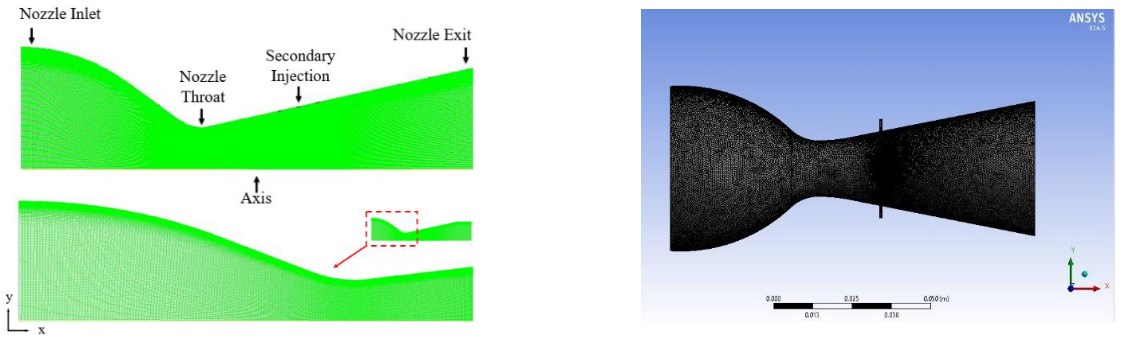
3. Computational Modeling and Simulation

This section covers the problem setup and boundary conditions used for CFD simulations. All CFD simulations were carried out in ANSYS Fluent software using the k-ϵ model to solve steady RANS equations, and data analysis was carried out using in-house developed performance codes. A non-premixed combustion model was utilized for modeling secondary combustion due to its capability of simulating high-speed reactions and turbulent diffusion flame. Additionally, the combustion model also allowed species prediction, the study of dissociation effects, and turbulence chemistry coupling [14].

For the current research, unstructured dense mesh generation was preferred over structured, since unstructured mesh reduces the overall complexity of the mesh generation and reduces computation time. The unstructured mesh was made using ANSYS ICEM with high grid resolution to capture the flow physics accurately, especially the combustion flame near injectors and oblique shock waves inside the nozzle. In the first instance, mesh sensitivity analysis was conducted using three mesh sizes, namely coarse-mesh A (approx. three million cells), medium-mesh B (approx. six million cells), and fine-mesh C (approx. 10 million cells), respectively. Mesh sensitivity was analyzed using three mesh sizes as given in

Table 4. Mesh details.

No.	Mesh Type	Mesh Size (Million)	Element Type
A	Coarse	3.0	Hexahedral
B	Medium	6.0	Hexahedral
C	Fine	10.0	Hexahedral

.

These meshes were very fine and were made up of hexahedral elements, which were tightly packed and clustered near the throat and divergent wall to capture flow properties near the wall. The mesh resolution is kept fine where large flow gradients are expected, such as at the wall and throat, whereas y+ was kept below 5.

To capture the secondary injection effect and its interaction with the flow, the grid was further refined in areas where the secondary injectors were located, as shown in Figure 4 below. To eliminate the near-wall effects, an inflation with a 1.5 mm thickness and five inflation layers was also applied. Some important mesh parameters are given in

Table 5. Mesh properties.

No.	Properties	Values	Units
1	Max thickness	1.5	mm
2	Number of layers	5	-
3	Aspect ratio	18.0	-
4	Max skewness ratio	0.78	-
5	Min orthogonal quality	0.56	-

.

Figure 5 presents the grid independence study in which the nozzle axial velocity is plotted against nozzle length for the three meshes. The grid independence study shows that there is a minor variation between all three meshes while the medium-mesh B trend almost gives the same result as the fine-mesh C. Thus, medium-mesh B was selected for further study. The outlet boundary was set as a pressure outlet at standard atmospheric conditions, whereas both the nozzle main inlet and secondary injection inlets were set as pressure inlets with the properties defined in

Table 6. Gas generator design properties.

Parameters	Value	Units
Nozzle inlet pressure	2	bar
Nozzle inlet temperature	1008	K
GOX injection pressure	2	bar
GOX injection temperature	300	K
GOX injection velocity	300	m/s
Nozzle outlet pressure	0.7	bar
Nozzle outlet temperature	800	K

.

Combusted species mass fraction from RP1 and LOX in the combustion chamber was used to model the reacting flow. The rocket propulsion analysis tool was utilized to acquire combusted species and their mass fractions. A total of nine species were obtained by combusting RP1 and LOX at standard atmospheric conditions. All the primary combusted species are mentioned in

Table 7. Species mass fractions.

No.	Species	Mass Fraction
1	C (gr)	0.4768273
2	C2H4	0.0000016
3	C2H6	0.0000123
4	CH4	0.1320777
5	CO	0.1579854
6	CO2	0.0644395
7	H2	0.0631787
8	H2O	0.1054770
9	HCHO	0.0000003

and their mass fractions were used in the non-premixed combustion model. Adiabatic heat transfers and no-slip conditions were assumed at the nozzle wall [15,16,17].

Initially, flow separation analysis was performed, and then GOX was injected into the divergent section. Upon stabilization of residuals and flow variables, post-processing was performed. Normal and tangential secondary injection techniques are then studied in comparison for the first time in GG for thrust regulation.

3.1. Flow Separation Analysis

The flow separation point (distance in the axial direction) was estimated empirically using Kalt and Badal and Schmucker flow separation criteria, which was about 37 mm aft of the throat [18,19]. To validate the flow separation point, a primary flow simulation of combusted species of RP1 and LOX was carried out without modeling combustion at sea level atmospheric conditions. It is seen from Figure 6 that the flow, after passing through the throat, expanded and detached from the wall of the nozzle, exactly at the location estimated using flow separation criteria.

The simulation also revealed a complicated shock formation, which was due to the flow adjustment to ambient pressure. The adverse pressure gradient caused the shock wave inside the nozzle, which separated the mainstream flow and boundary layer from the nozzle wall. Due to over-expansion and over-compression, a repeated diamond shock, a triple point, an incident shock, a Mach disk, and a reflected shock were also observed, as shown in Figure 6. These results were validated by Balabel’s convergent–divergent rocket nozzle, Munday, and Gvozdeva gas flow in nozzles, as they obtained the same diamond shock pattern formation through CFD. The recirculation region that originated from the flow separation was utilized for a secondary injection of GOX and modeling combustion [20,21,22].

3.2. Secondary Injection Analysis

Table 8. Graph label description.

Configuration Label	Injection Type	Injector Location (mm)	Mass Flow (kg/s)
C1 N 20 mm 0.006 kg/s: C1	Normal: N	20	0.006
C2 T 20 mm 0.006 kg/s: C2	Tangential: T	20	0.006
C3 N 37 mm 0.006 kg/s: C3	Normal: N	37	0.006
C4 T 37 mm 0.006 kg/s: C4	Tangential: T	37	0.006

describes the labels used in the graphs given in further sections.

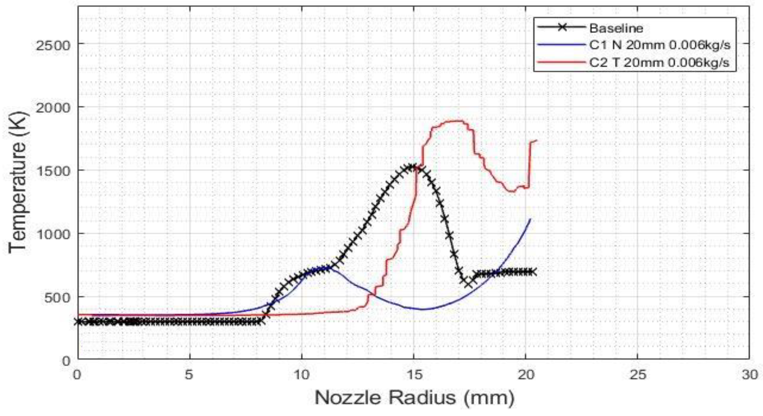
3.2.1. Configuration C1 and C2: Effect of Temperature

Figure 7 shows the static temperature plotted against the nozzle radial length. It can be seen that C1 shows a gradual rise in temperature, whereas C2 shows a sudden temperature rise. This is because when the GOX is injected normally, as shown in Figure 8b, it is unable to penetrate the core flow, resulting in weak but stable combustion near the injector, whereas with tangential injection, as shown in Figure 8d, the GOX is injected parallel to the core flow, allowing it to be dragged downstream, causing combustion along the flow.

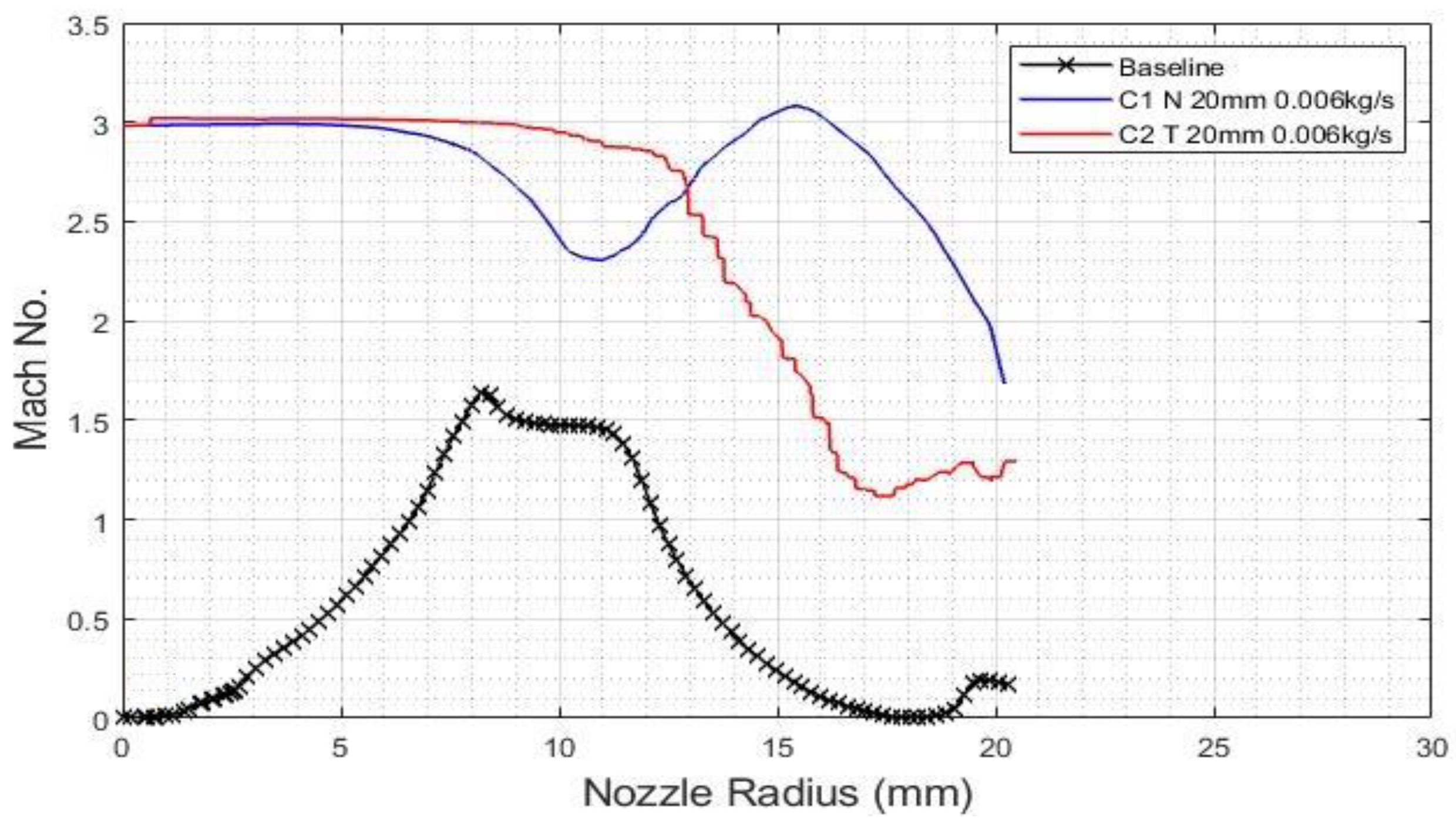
3.2.2. Configuration C1 and C2: Effect of Mach Number

Figure 8a,c and Figure 9, show the exit Mach number profiles and contours. In both configurations, the secondary combustion has reenergized the core flow, as can be seen from the increased Mach number in Figure 8a,c. A reduction in the Mach number of C2 was observed in the outer periphery of the nozzle from 12 mm to 18 mm, which was due to the combustion and the presence of the streamlined flame in the region.

3.2.3. Configuration C3 and C4: Effect of Temperature

The same 1 mm normal and tangent injectors were then placed 37 mm aft of the throat at the flow separation point. It was expected that injecting GOX at the flow separation point would allow GOX to mix with the shear layer of the core flow. It was revealed that the C3 performed better than the C4 in terms of mixing and rapid temperature rise, as evident from Figure 10b,d and Figure 11 GOX tangential injection in C4 was not able to cause combustion efficiently as there was no significant temperature rise observed from Figure 10b,d and Figure 11.

3.2.4. Configuration C3 and C4: Effect of Mach Number

The Mach number profile of C3 in Figure 10a and Figure 12 dropped but remained supersonic. The rise in the Mach number of C4 in Figure 10c and Figure 12 was not due to combustion but to unconsumed GOX exiting the nozzle from the four tangential injectors.

Configuration C1 gave sustained combustion and a Mach number. It was found that injecting GOX normally at 300 m/s with a mass flow rate of 0.006 kg/s before the flow separation point gave a stable flame, with the temperature reaching up to a maximum of 1200 K. The detached flow re-energized, accelerated, and filled the void space with combusted gases. The nozzle became highly supersonic from the center to the outer region of the nozzle, i.e., from 0 to 21 mm. The flow remained between Mach 1.5 and Mach 3.0.

Injecting GOX normally allowed GOX to penetrate and mix with the core flow efficiently, while the symmetry of the flow was also maintained, unlike other configurations. This Mach enhancement led to an increase in shaft power of the turbine, which increases propellant flow rate in the main chamber correspondingly with pump power. Hence, the thrust of the main engine increases.

Based on configuration C1, the prototype was manufactured with normal secondary injection ports, and an experiment was conducted to validate CFD results.

4. Experimental Setup

The experimental setup was established to perform the required research and development. A schematic in Figure 13 shows the process and instrumentation diagram of the experimental setup.

Table 9. Specifications of experimental apparatus.

No.	Apparatus	Details	Quantity
1	Pressure tanks	N2, 152 bar, 90 Liters	2
2	Data acquisition	Arduino 2560, ATmega2560, 6–20 V	2
3	Ignition mechanism	Spark Plug-Electrical Coil, 12-volts	1
4	Flow meter gauges	Pressure 200 bar, Temperature 366.15 K	5
5	Emergency stop	Kill Switch DPST-NC, 250 V, Max 338 K	1
6	Pressure sensors	HPT300-S, 0 to 600 bar, 308–398.15 K	5
7	Temperature sensors	K-Type, 73.15–1623.15 K	5
8	Chamber/nozzle	AISI 1018 Carbon St, Melt Temp 1093 K	1
9	Primary injectors	Co Axial Plate, Max Mdot 0.113 Kg/s	1
10	Secondary injectors	Normal, Max Dia 1 mm Each	4
11	Fuel tank	Kerosene, 150 bar, 20 Liters	1
12	First oxidizer tank	LOX, 150 bar, 82.5 Liters	1
13	Second oxidizer tank	GOX, 150 bar, 82.5 Liters	1

presents details of specification of the experimental apparatus.

GG, along with the injection head and combustion chamber, is shown in Figure 14a. Figure 14b shows an integrated GG with propellant tanks on the test bed along with the required data acquisition systems. A spark plug-based ignition system was used to ignite the propellants for primary combustion. Convergent and divergent parts of the nozzle were water-cooled. Five pressure and three temperature ports were strategically placed to evaluate the experimental performance. Piezoelectric pressure sensors and K-Type thermocouples were used to measure these parameters.

To obtain data from the sensors, a reliable data acquisition method for collecting and processing information was mandatory. An Arduino was selected for data acquisition from the sensors. Figure 15, depicts two Arduino Mega 2560 hardware components that were integrated and programmed on the Vero Board.

Thermocouples, which are electrical devices, were used to obtain the temperature profiles at the aft section of the engine. The most common type of thermocouple is the “K-Type” (chromel–alumel) thermocouple, which was used for this experiment. The K-Type is the most commonly used general-purpose thermocouple, with a sensitivity of approximately 41 μV/°C. The K-Type thermocouples were readily available in the propulsion lab, and they fulfilled the required range of temperature variation from −200 °C to +130 °C (73.15 K to +1623.15 K) needed for the experiment.

To measure the pressure profile, piezoelectric pressure sensors “HPT300-S Universal Pressure Sensors by Holykell Technology” were used in the experiment. The reason for choosing HPT300-S for measuring pressure is its rugged design. It also provides vibration resistance, and shock resistance, has a wide range of temperature variations, and is suitable for other extreme environmental conditions. At standard conditions (ambient temperature: 25 °C), the working pressure and temperature of HPT300-S sensors are 0 bar–600 bar and 35 °C to +125 °C (308.15 K to +398.15 K), respectively, while the measuring error and accuracy are approximately 1.0 to 3% F.S. The HPT300-S sensors were lightweight, small in size, easy to install and operate, and fulfilled experimental requirements, so they were considered for the experiment. Figure 16, below, shows both thermocouples and pressure sensors.

4.1. Experiment Boundary Conditions

Experiments with and without secondary injection of GOX were carried out. The primary objective of the experiment was to validate CFD simulation data. The boundary conditions of the test are given in

Table 10. Boundary conditions of the test.

Parameters	Value	Units
Primary combustion pressure	2	bar
Primary combustion temperature	1008	K
Secondary injection GOX mass flow rate	0.006	kg/s
Secondary injection GOX velocity	300	m/s

.

Figure 17a shows the exhaust plume before the initiation of secondary injection. The plume before the secondary injection of GOX was small and unstable, indicating that the flow was separated from the nozzle wall due to the large nozzle expansion ratio. Whereas in Figure 17b, the flow inside the nozzle reenergized and gained momentum following the start of the secondary injection of GOX. Injection of GOX inside the divergent section of the nozzle, before the flow separation point, caused GOX to mix successfully with the fuel-rich flow, causing combustion inside the nozzle. Moreover, due to secondary combustion, the flow accelerated and the plume became turbulent, as can be seen in Figure 17b. The experimental data from C1’s experiments were collected and analyzed. The next section discusses the data obtained from the experiment.

4.2. Experimental Test Results and Discussion

4.2.1. Primary Combustion Chamber Pressure “Pc”

Figure 18 shows Test 1 and Test 2 combustion pressure measured against time for 15 s without secondary combustion. It was noted that a combustion pressure of 200,000 Pascal (2 bars) was maintained from 5 s to 12 s, confirming consistency and reliability.

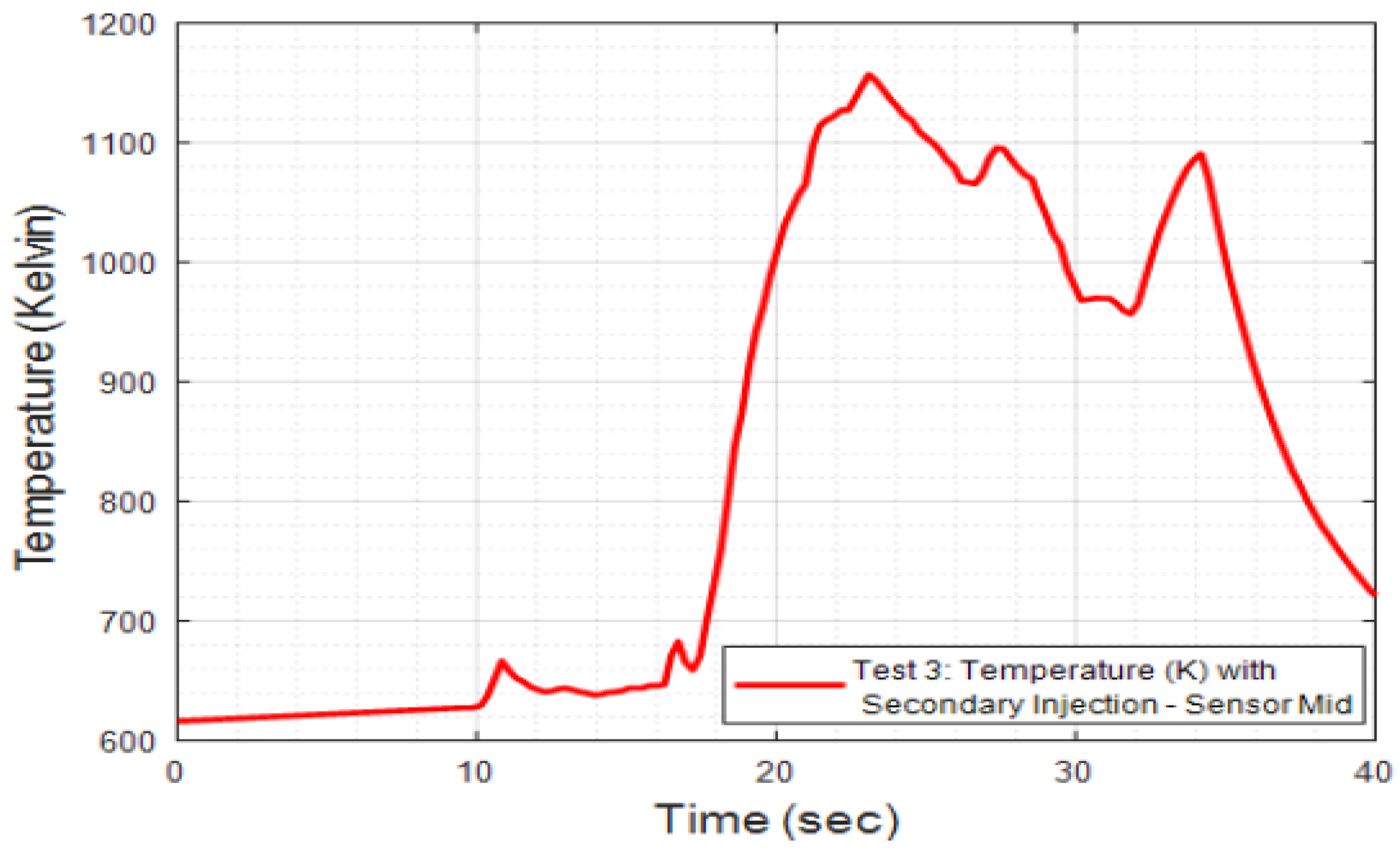
4.2.2. Nozzle Temperature Profile with Secondary Injection

Figure 19 shows Test 3’s secondary combustion temperature, in which secondary injection was initiated. The burn time duration of the test was 35 s, which was kept longer to establish the flow in the nozzle and to sustain secondary combustion. It can be seen from Figure 19 that the temperature rose gradually from 0 to 15 s. This gradual rise was because of GOX injection effects and flow settling time in the nozzle. The injection temperature of GOX was 300 K, and there was also a possibility of GOX making a boundary layer over the region where the thermocouples were axially placed. After 15 s, the temperature inside the nozzle increased abruptly, indicating settled flow and sustained combustion. The secondary combustion was sustained for another 15 s, giving a temperature range from 950 K to 1150 K.

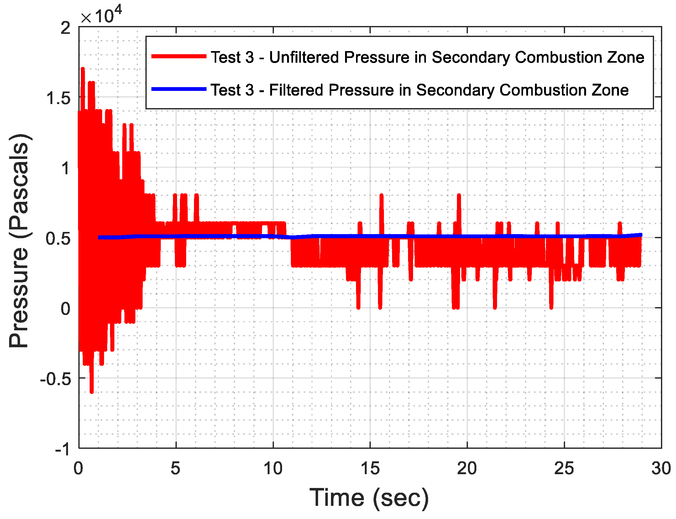
4.2.3. Nozzle Pressure Profile with Secondary Injection

Figure 20 shows Test 3’s secondary combustion pressure inside TAN with a second injection of GOX. The secondary combustion pressure presented in Figure 20 was also filtered to eliminate unwanted data entries. An initial rise in pressure was observed, ranging up to 150,000 Pascal (1.5 bar) from 0 to 5 s. This sudden pressure overshoot is usually observed in liquid propulsion rocket engines, which is caused by the startup ignition transient and initial combustion reaction in the primary combustion chamber. After 5 s, secondary combustion stabilized and the combustion pressure settled for the rest of the burn time. The secondary combustion pressure inside the nozzle ranged from 30,000 to 50,000 Pascal (0.3 bar to 0.5 bar).

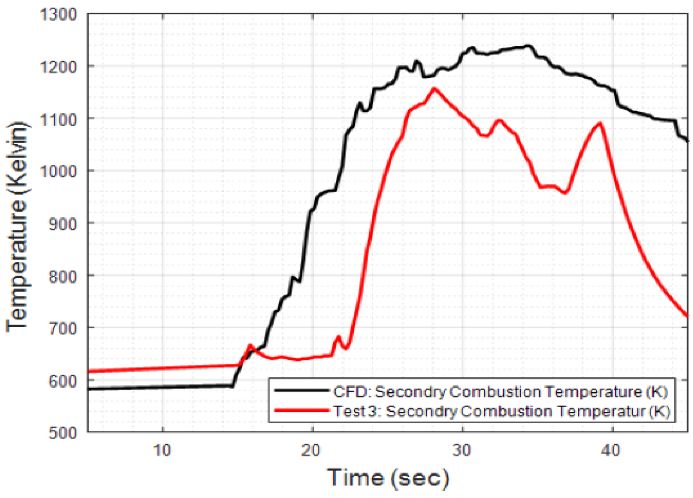
4.2.4. Experimental Test Results Validation with CFD

For validation of experimental results and data, CFD simulation data was compared. Figure 21 and Figure 22 show a comparison of secondary combustion pressure and temperature. It can be seen that both secondary temperature and pressure obtained from CFD simulation are in agreement with the experimental data. Experimental and CFD simulation percentage error is discussed in forthcoming Section 4.2.6.

4.2.5. Instrumentation Error and Calibration

The pressure sensors (HPT300-S) and thermocouples (K-Type) were all acquired from the supplier as per stated precision standards. Before the experiment, all the possible sources of errors associated with the instrumentation were outlined for calibration and data acquisition errors. For pressure sensors, hysteresis and non-uniformity estimation activities were carried out, and all sensors were calibrated, using a precision electronic calibrator as a reference. All errors that occurred during calibration were reduced by performing the calibration under test conditions. For thermocouples, two methods: the stirred bath method and the block calibrator method, were employed for calibration.

4.2.6. Experimental and CFD Simulation Percentage Error

A percent error was estimated, which is the difference between experimental and CFD simulation data in terms of a percentage value. The percentage errors of temperature and pressure were estimated at various time intervals using the following relation:

Pe% = (Mv − Tv/Tv) ∗ 100%

where Pe is the percentage error, Mv is the measured value, and Tv is the theoretical value. From Figure 23 below, it can be seen that after 5 s of burn time the percentage error in the case of pressure is reduced to a minimum of 3%. In the case of temperature, the percentage error reduces from 30% to a minimum of 6% after 10 s of burn time. The reason for this initial 30% rise in percentage error is temperature variation around the reference junction, which was caused by the LOX exiting the nozzle before the actual hot fire. LOX was allowed to flow through the engine before the hot test fire so that the pressure and temperature inside the LOX tank could be maintained.

5. Chemical Equilibrium

Products obtained from reacting LOX/RP-1 are used as reactants for secondary combustion reactions, and final product species are obtained. The compositions of different species at equilibrium are determined by minimizing the Gibbs free energy of the system. Minimization has been done using the method of steepest descent and the results obtained were refined by the Nelder–Mead method [23,24,25].

Species after secondary combustion were also obtained from CFD simulations. The mass fractions of these species were compared with the mass fractions of chemical equilibrium calculations and validated accordingly.

5.1. Gibbs Free Energy

The procedure to calculate Gibbs energy of a reacting system is fairly standard and is briefly explained here: Gibbs energy of the system is written as G.

$$G={\displaystyle \sum }_{i=1}^m{\mu }_i{n}_i$$

(1)

The objective is to minimize Gibbs energy subject to mass balance constraints. Constraints can be included using Lagrangian multipliers resulting in a modified function G′.

$$G^{\prime }={\displaystyle \sum }_{i=1}^m{\mu }_i{n}_i+{\displaystyle \sum }_{j=1}^l{\lambda }_j\left({\displaystyle \sum }_{i=1}^m{n}_i{\beta }_{ij}-b_j\right)$$

(2)

The formula coefficient matrix is known as β. For a system containing the species CH₄, H₂O, H₂, CO, and CO₂, it can be written as:

$$\beta =\begin{array}{cc}& \begin{array}{ccc}C& H& O\end{array}\\ \begin{array}{c}C{H}_4\\ H_{2}O\\ H_2\\ CO\\ C{O}_2\end{array}& \left[\begin{array}{ccc}1& 4& 0\\ 0& 2& 1\\ 0& 2& 0\\ 1& 0& 1\\ 1& 0& 2\end{array}\right]\end{array}$$

(3)

The column vector b represents moles of elements in the input stream.

$$b=\begin{array}{c}C\\ H\\ O\end{array}\left[\begin{array}{c}{n}_C\\ n_H\\ n_O\end{array}\right]$$

(4)

Mass balance is then written as:

$$\left[\begin{array}{ccccc}{n}_{C{H}_4}& n_{H_{2}O}& n_{H_2}& n_{CO}& n_{C{O}_2}\end{array}\right]\left[\begin{array}{ccc}1& 4& 0\\ 0& 2& 1\\ 0& 2& 0\\ 1& 0& 1\\ 1& 0& 2\end{array}\right]=\left[\begin{array}{ccc}{n}_C& n_H& n_O\end{array}\right]$$

(5)

The chemical potential of ideal gas species can be written as:

$${\mu }_i=g_i^o+RT\ln \left(y_{i}P\right)$$

(6)

Mass Balance Constraints

When λ_j are taken as Lagrangian multipliers, they are treated as variables along with n_i values. However, they can be fixed as constants and treat λ_j as penalty factors. The penalty method has been used to handle the mass balance constraints [26].

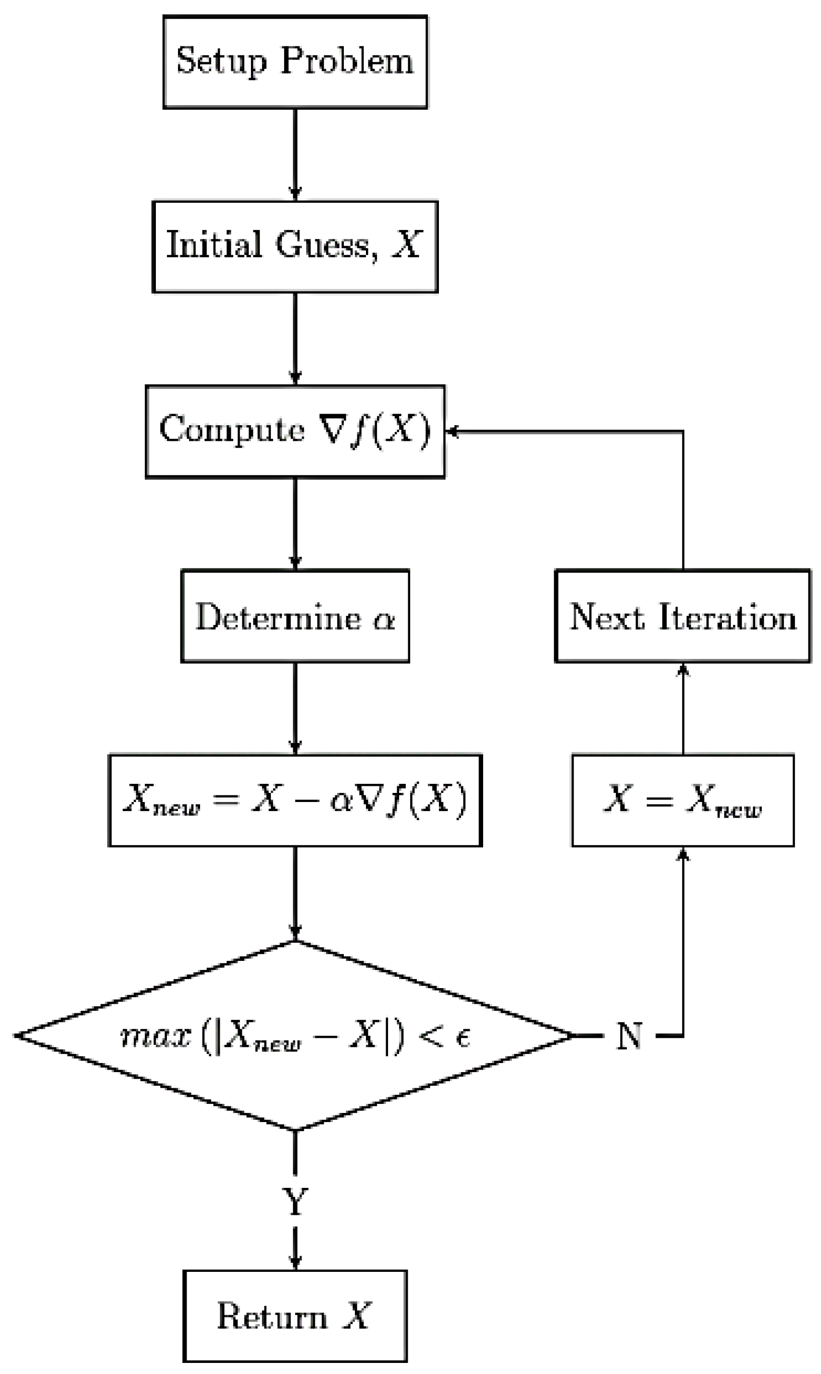
5.2. Method of Steepest Descent

The method of steepest descent has been used to find the minimum of Gibbs energy. The flow chart is shown in Figure 24. Each operation is explained in this section.

5.2.1. Setup Problem

• Set T and P of the problem.
• Set the species involved by setting the formula coefficient matrix, β.
• Set initial composition. Calculate the number of moles of each element and set the vector, b.

5.2.2. Initial Guess, X

Assume n_i of the species present in the product stream. Call this vector X.

5.2.3. Compute ∇f(X)

Derivatives (∂G′)/(∂n_i) are calculated numerically using centered difference.

$$f_i=\frac{\partial G^{\prime }}{\partial n_i}=\frac{G^{\prime }\left(n_i+d\right)-G^{\prime }\left(n_i-d\right)}{2d }, i=1,N$$

(7)

where d is a small number (10⁻⁸). This function generates a vector of the first derivatives of the cost function w.r.t. n_i variables.

5.2.4. Determine α

In the method of steepest descent, the solution vector is moved in a direct negative of the derivative.

$$X_{new}=X-\mathsf{\alpha }\nabla f\left(X\right)$$

(8)

However, the value of the derivative needs to be scaled down. The usual practice is to take α as a very small number, such as 10⁻⁶. However, the scale factor α needs to be determined by hit and trial. A method to fix this value adaptively has been devised for this work by fixing a maximum of the allowed step.

• Find the maximum of the derivatives computed.

maxF = max(abs(∇f))

• Fix the maximum allowable step in the variables.

maxStep = 1.0e⁻⁴

• If maxF > maxStep, fix α = maxStep/maxF. Otherwise, take α = 1.

5.2.5. Check for Convergence

If the max change (in any of the variables) is less than ϵ = 10^−4, stop the iterations and return the answer. Otherwise, replace X with X_new and repeat the iteration.

6. Combustion Species

Figure 25 shows the mass fraction of combustion species obtained from CFD along the axial length of the GG divergent section. These species are the products of secondary combustion with GOX. Pre-heated primary combustion products react with gaseous oxygen to produce these species.

Table 11. Species mass fraction (CFD) and chemical equilibrium calculations at exit plane of GG.

No.	Species	Mass Fractions
		CFD	Chemical Equilibrium
1	C (gr)	0.39412	0.388
2	CH4	0.10917	0.15
3	CO	0.13127	0.12
4	H2O	0.10302	0.098
5	CO2	0.0942	0.102
6	H2	0.05223	0.054
7	O2	0.113	0.099

gives the comparison of species obtained from CFD and chemical equilibrium calculations in Python. From this table, it can be seen that species calculated through Gibbs free energy minimization follow the species obtained from the CFD results; hence, validating the CFD simulations.

7. Performance Evaluation

The performance of the rocket engine and the nozzle is dependent on parameters such as thrust (T), specific impulse (I_sp), thrust-specific fuel consumption (TSFC), thermal efficiency (η_th), propulsive efficiency (η_p), and overall efficiency (η_o). This section includes the estimation of all the mentioned parameters and presents a performance comparison of configuration C1 with the baseline configuration [27,28,29].

Figure 26 and Figure 27 represent the trend of thrust and a specific impulse of configuration C1 and baseline configuration. It was observed that about 42% of thrust increments and 46% of specific impulse increments were achieved at sea level. The thrust and specific impulse were enhanced, ranging from centerline 0 to 21 mm.

Another important parameter to evaluate performance is the specific fuel consumption (SFC), which defines how efficiently a rocket engine converts chemical energy into power or useful energy. It is the mass of fuel required to provide the net thrust for a given time. The SFC of C1 was estimated and presented in Figure 28a. It is observed that in C1 fuel consumption increased from 14 mm to 21 mm, which indicates the fuel is being consumed and being burnt efficiently, radially [30,31,32].

The efficiency of a rocket engine is described as internal and external efficiency. Internal efficiency is called thermal efficiency, whereas external efficiency is called propulsive efficiency, and a combination of both efficiencies is known as the overall efficiency of the system [26]. Figure 28b–d shows estimates of C1’s thermal, propulsive, and overall efficiency plotted against the baseline configuration.

Thermal efficiency specifies the effectiveness of converting power input into the system into power output. Figure 28b shows the trend of thermal efficiency versus nozzle radius with and without thrust regulation via GG. It is observed that the thermal efficiency is increased by about 24% from 0 mm to 21 mm radially.

The propulsive efficiency was estimated against a Delta-V (∆V) of 1 km/s, equivalent to a rocket travelling at Mach 3. Figure 28c plots the trend of propulsive efficiency against the ratio V/C, which is the ratio of rocket flight velocity (V) to exhaust velocity (C). It can be seen from the plot that 100% propulsive efficiency can be achieved in both cases and the rocket can be operated with an exhaust velocity less than its flight velocity. However, with thrust regulation in GG, V/C can be extended up to a ratio from 0 to 1.7.

Figure 28d plots overall efficiency versus nozzle radius. Figure 28d shows that without thrust regulation, overall efficiency could reach 10% and was distributed erratically along the nozzle radius. While with thrust regulation, the overall efficiency increased by up to 24% and was highest in the region from 0 mm to 10 mm.

8. Conclusions

To achieve thrust regulation through GG, the effect of secondary GOX injection in the RP1-rich jet was investigated. A total of four cases of GOX injection were studied, involving normal and tangential injection techniques and injection location as a variable. The computational data presented show that, in practice, the normal injection technique supersedes the tangential technique. The comparison of CFD and experimental data revealed a strong correlation between simulations and experiments. Chemical equilibrium calculations were also in good agreement with the CFD results of the combustion species.

It was observed that the GG performance was greatest when GOX is injected normally at 90°, from a position located 20 mm aft of the throat, with an injection velocity of 300 m/s. These injection parameters allowed the GOX to penetrate and mix with unburnt RP1 more efficiently.

Normal injection technique operating at sea level resulted in a 42% increase in thrust and a 46% increase in specific impulse. The increment in thrust is dependent on the injection position. Additionally, a stronger combustion flame inside the secondary combustion zone results in greater exhaust velocity. Stronger combustion displaces the exhaust jet towards the centerline and reduces the expansion ratio, instigating an increase in the exit Mach number. This gives increased turbine shaft power, hence increasing the mass flow in the main chamber, resulting in the increased thrust of the engine. Thus, thrust regulation of the main engine is achieved through secondary combustion in GG.

References

1. De Almeida, D.S.; Maria, C.; Pagliuco, D.M. Development Status of L75: A Brazilian Liquid Propellant Rocket Engine. J. Aerosp. Technol. Manag. 2014, 6, 475–484. [Google Scholar] [CrossRef] [Green Version]
2. Citarella, R.; Ferraiuolo, M.; Perrella, M. Thermostructural Numerical Analysis of the Thrust Chamber of a Liquid Propellant Rocket Engine. Materials 2022, 15, 5427. [Google Scholar] [CrossRef]
3. Bulman, M.J. Rocket vehicle thrust augmentation within divergent section of nozzle. U.S. Patent US6568171B2, 5 July 2002. [Google Scholar]
4. Borowski, S.; Dudzinski, L.; McGuire, M. Vehicle and Mission Design Options for the Human Exploration of Mars/Phobos Using Bimodal NTR and LANTR Propulsion. In Proceedings of the AIAA, Cleveland, OH, USA, 13–15 July 1998. [Google Scholar]
5. Shen, J.; Yu, Y.; Liu, X.; Cao, J. Experimental Research on Microwave Ignition and Combustion Characteristics of ADN-Based Liquid Propellant. Micromachines 2022, 13, 510. [Google Scholar] [CrossRef] [PubMed]
6. Li, J.; Liu, K.; Gao, Y.; Liu, S.; Wang, W.; Liu, Y. Combustion Characteristics Experimental Study of Solid Hydrocarbon Propellant for Air-Turbo Rocket. J. Propuls. Power 2018, 34, 1198–1205. [Google Scholar] [CrossRef]
7. Shynkarenko, O.; Gontijo, M. Development of a Thrust Control System for Rocket Engines. In Proceedings of the Conference: 71st International Astronautical Congress (IAC 2020), Online, 12–14 October 2020. [Google Scholar]
8. Liquid Propellant Gas Generators; NASA Space Vehicle Design Criteria (Chemical), NASA SP-8081; NASA Lewis Research Center: Cleveland, OH, USA, 1972; p. 110.
9. Cha, J. A Study on Thrust Control System Design for Multi-Nozzle Solid Propulsion System. Master’s Thesis, Department of Aerospace and Mechanical Engineering, Korea Aerospace University, Goyang, Korea, 2014. [Google Scholar]
10. Mohammed, S.; Badi, M. Static Testing Of Hybrid Rocket Engine Using Biomass College of Engineering. 2022. Available online: https://scholarworks.uaeu.ac.ae/all_theses/930 (accessed on 15 August 2022).
11. Lee, D.; Lee, C. Secondary combustion in a staged hybrid rocket engine. J. Mech. Sci. Technol. 2017, 31, 3067–3073. [Google Scholar] [CrossRef]
12. Marshall, J.H. Thrust Augmented Nozzle for a Hybrid Rocket with a Helical Fuel Port. Ph.D. Thesis, Utah State University, Logan, UT, USA, 2018. [Google Scholar]
13. Sutton, G.P. Rocket Propulsion Elements, 7th ed.; Wiley: Hoboken, NJ, USA, 2000; ISBN 0471326429. [Google Scholar]
14. Pouransari, Z. Fundamental Studies of Non-Premixed Combustion in Turbulent Wall Jets Using Direct Numerical Simulation. Doctoral Dissertation, KTH Royal Institute of Technology, Stockholm, Sweden, 2011. [Google Scholar]
15. Ponomarenko, A. RPA—Tool for Rocket Propulsion Analysis. 2014. Available online: http://www.rocket-propulsion.info/resources/software/rpa/RPA_LiquidRocketEngineAnalysis.pdf (accessed on 10 September 2022).
16. Ponomarenko, A. Estimation of Engine Mass. 2015, pp. 1–10. Available online: http://w.lpre.de/downloads/2/docs/RPA_EstimationOfEngineMass.pdf (accessed on 10 September 2022).
17. Ponomarenko, A. Assessment of Delivered Performance of Thrust Chamber. 2013. Available online: http://w.lpre.de/downloads/2/docs/RPA_AssessmentOfDeliveredPerformance.pdf (accessed on 9 September 2022).
18. Kalt, S.; Badal, D.L. Conical rocket nozzle performance under flow- separated conditions. J. Spacecr. Rocket. 1965, 2, 447–449. [Google Scholar] [CrossRef]
19. Stark, R. Flow Separation in Rocket Nozzles, a Simple Criteria. In Proceedings of the 41st AIAA/ASME/SAE/ASEE Joint Propulsion Conference & Exhibit, Tucson, AZ, USA, 10–13 July 2005. [Google Scholar] [CrossRef] [Green Version]
20. Balabel, A.; Hegab, A.M.; Nasr, M.; El-Behery, S.M. Assessment of turbulence modeling for gas flow in two-dimensional convergent–divergent rocket nozzle. Appl. Math. Model. 2011, 35, 3408–3422. [Google Scholar] [CrossRef]
21. Munday, D.R.; Gutmark, E.J.; Liu, J.; Kailasanath, K. Flow and Acoustic Radiation from Realistic Tactical Jet CD nozzles. In Proceedings of the 14th AIAA/CEAS Aeroacoustics Conference (29th AIAA Aeroacoustics Conference), Vancouver, BC, Canada, 5–7 May 2008. [Google Scholar]
22. Gvozdeva, L.G.; Chulyunin, A.Y. Numerical study of the gas flow in nozzles and supersonic jets for different values of specific heats. J. Phys. Conf. Ser. 2015, 653, 12068. [Google Scholar] [CrossRef] [Green Version]
23. Olsson, D.M.; Nelson, L.S. The Nelder-Mead Simplex Procedure for Function Minimization. Technometrics 1975, 17, 45–51. [Google Scholar] [CrossRef]
24. Yang, S. Descent Method—Steepest Descent and Conjugate Gradient, towards Data Science. 2020. Available online: https://towardsdatascience.com/descent-method-steepest-descent-and-conjugate-gradient-math-explained-78601d8df3ce (accessed on 10 September 2022).
25. Koretsky, M.D. Engineering and Chemical Thermodynamics, 2nd ed.; John Wiley & Sons: Hoboken, NJ, USA, 2012; ISBN 978-0-470-25961-0. [Google Scholar]
26. Liu, G.R.; Quek, S.S. The Finite Element Method—A Practical Course, 2nd ed.; Butterworth-Heinemann: Oxford, UK, 2013; ISBN 0-7506-5866-5. [Google Scholar]
27. Cantwell, B.J. Aircraft and Rocket Propulsion; Stanford University: Stanford, CA, USA, 2021. [Google Scholar]
28. Cha, J.; de Oliveira, É.J. Performance Comparison of Control Strategies for a Variable-Thrust Solid-Propellant Rocket Motor. Aerospace 2022, 9, 325. [Google Scholar] [CrossRef]
29. Pizzarelli, M. Overview and analysis of the experimentally measured throat heat transfer in liquid rocket engine thrust chambers. Acta Astronaut. 2021, 184, 46–58. [Google Scholar] [CrossRef]
30. Mattingly, J.D. Elements of Propulsion: Gas Turbines and Rockets; American Institute of Aeronautics and Astronautics: Reston, VA, USA, 2006; ISBN 1563477793. [Google Scholar]
31. Tarifa, M.C.; Pizzuti, L.; Bernardo, S.; Bernardo, S. Theoretical Performance Analysis of Hybrid Rocket Propellants Aiming at The Design of a Test Bench and a Propulsive. In Proceedings of the 8th European Conference for Aeronautics and Space Sciences, Madrid, Spain, 1–4 July 2019. [Google Scholar]
32. Yang, V. Liquid-Propellant Rocket Engine Injector Dynamics and Combustion Processes at Supercritical Conditions; The Pennsylvania State University: State College, PA, USA, 2004. [Google Scholar]
Figure 1. Flow chart for a gas generator LPRE cycle calculation.
Applsci 12 10563 g001
Figure 2. Geometric parameters of gas generator nozzle with secondary injection positions, whereas x-si1 and x-si2 are secondary injection positions (dimensions in mm).
Applsci 12 10563 g002
Figure 3. Gas generator configurations: (a) normal injectors; (b) tangent injectors.
Applsci 12 10563 g003
Figure 4. Mesh B—used for CFD simulations.
Applsci 12 10563 g004
Figure 5. Grid independence study.
Applsci 12 10563 g005
Figure 6. Contour of Mach number showing flow separation point and Mach disk.
Applsci 12 10563 g006
Figure 7. Static temperature vs. nozzle radius for C1 and C2.
Applsci 12 10563 g007
Figure 8. (a,b) Normal injection-Mach number and static temperature. (c,d) Tangent injection-Mach number and static temperature contours.
Applsci 12 10563 g008
Figure 9. Mach no. vs. nozzle radius of C1 and C2.
Applsci 12 10563 g009
Figure 10. (a,b) Normal injection-Mach number and static temperature. (c,d) Tangent injection-Mach number and static temperature.
Applsci 12 10563 g010
Figure 11. Static temperature vs. nozzle radius of C3 and C4.
Applsci 12 10563 g011
Figure 12. Mach number vs. nozzle radius of C3 and C4.
Applsci 12 10563 g012
Figure 13. Process and instrumentation layout of the experimental setup.
Applsci 12 10563 g013
Figure 14. (a) Gas generator major components. (b) Gas generator with configured instrumentation.
Applsci 12 10563 g014
Figure 15. Arduino Mega 2560 integrated on Vero board for data acquisition.
Applsci 12 10563 g015
Figure 16. Thermocouples and pressure sensors.
Applsci 12 10563 g016
Figure 17. Exhaust plume of GG: (a) without secondary combustion; (b) with secondary combustion.
Applsci 12 10563 g017
Figure 18. Test 1 and Test 2, combustion chamber pressure vs. burn time.
Applsci 12 10563 g018
Figure 19. Temperature vs. burn time.
Applsci 12 10563 g019
Figure 20. Pressure in Secondary Combustion Zone vs. Burn Time.
Applsci 12 10563 g020
Figure 21. Comparison of Secondary Combustion Pressure.
Applsci 12 10563 g021
Figure 22. Comparison of secondary combustion temperature.
Applsci 12 10563 g022
Figure 23. Percentage error between CFD and experimental data.
Applsci 12 10563 g023
Figure 24. Flow chart of method of steepest descent.
Applsci 12 10563 g024
Figure 25. Mass fraction of combustion species obtained from CFD.
Applsci 12 10563 g025
Figure 26. Thrust vs. nozzle radius.
Applsci 12 10563 g026
Figure 27. Isp vs. nozzle radius.
Applsci 12 10563 g027
Figure 28. (a) Specific fuel consumption. (b) Thermal efficiency. (c) Propulsive efficiency. (d) Overall efficiency.
Applsci 12 10563 g028