Optimizing Transportation between Sea Ports and Regions by Road Transport and Rail and Inland Waterway Transport Means Including “Last Mile” Solutions

Abstract

Optimization transportation cargo and passengers between ports and regions are very important, because industrial regions are located some distance from ports. The demand for energy request for the movement of transport is a necessity in the modern world. Transport and activity called transportation are used daily, everywhere, and a lot of energy is needed to power the various transport modes. Today different transport modes are being used to transport passengers and cargo. It is quite common to use road transport, which can transport passengers and cargo from door to door. Considering alternative possibilities (road, railway and/or inland waterway transport), it is important, based on theoretical and experimentation, to identify optimal solutions. In finding transport modes that are either most technically or economically effective, we could unearth possible solutions which would require minimal energy use. Unfortunately, with increased transportation, this often leads to traffic congestion on the roads, which requires additional energy (fuel). This situation generates requirements from many stakeholders in terms of finding ways to decrease the transportation time and energy (fuel) consumed by transport modes. A theoretical method evaluation is conducted on the optimal transportation possibility that minimizes transportation time and energy (fuel) use by employing graph theory, which is presented in this paper. The scientific contribution is the development of a transport modes comparative index, which is then used for evaluations. This paper presents possible alternative transportation conditions based on a multi-criteria evaluation system, proposes a theoretical basis for the optimal solutions from an eco-economic perspective that considers energy, and provides for experimental testing during a specific case study. The final results from the case study provide recommendations and conclusions.

1. Introduction

Sea transport is one of the main drivers of the global economy. Energy demands are increasing worldwide, and the biggest consumer of energy is transportation. About 80% of the cargo in the world is transported by sea transport within different regions [1]. At the same time, industrial areas (e.g., hinterland) are often located long distances from the ports; the “Ruhr” area in Germany, which is the largest industrial area, is located up to 250–400 km from the main West European ports, such as Antwerp, Rotterdam, Hamburg, etc. Similar situations regarding long distances between industrial areas and ports are observed in many other European and global regions.

Decreasing energy consumption due to optimization of the cargo transportation processes between regions, ports and industrial regions is viewed to be a very important research direction, as it has a significant impact on society. The total energy demand in the world is about 173,340 TWh [1]; at the same time, transport consumption is about 25% of the total energy consumption [2]. Increasing energy prices are being demanded globally by many transportation processes seeking to optimize the decrease in energy through transportation [3]. Optimization of transportation processes and decreasing energy (fuel) demands today are viewed as some of the main challenges for industries and society in general. Optimizing transport processes that considers reducing energy demand is argued to be one of the key challenges for research and application, which is the main aim of this paper.

Road transport is being used very intensively, because of the flexibility in using this transport mode to deliver cargo between regions, from ports to cargo destination places or transport cargo from shippers to ports or other areas. At the same time, road transport has its limitations, such as capacity and relatively high engine power used, as a result of which high fuel consumption occurs, which is not optimal compared to other alternatives [3,4].

Railway transport links many regions, ports and cargo consignees’ locations and is often used to transport cargo between regions, from port to its destination places or from shippers’ location. Railway transport has sufficient capacity and requires less energy in comparison with road transport for the same quantities of cargo transportation, but at the same time, in most cases, it cannot be used for door-to-door transportation [5,6,7].

Traffic congestion on the roads, and especially in urban areas, often increases transportation costs and energy consumption, which generates requests for studies to find optimal transportation solutions and decrease energy for transportation tasks.

In many countries, inland waterway transport connects areas and seaports with inland industrial and population concentration regions and can be used for cargo delivery between areas, from port to its destination areas and from shippers’ areas to the ports. Inland waterway transport (barges and inland waterways cargo ships) in many cases uses less energy (fuel) consumption for the transportation of the same cargo volumes [8,9,10].

Today, there are many methods for assessing optimal transport modes between regions, consignors and consignees, including energy savings; but at the same time, many of them do not allow for a complex assessment of optimal transport and application impacts in difficult transport conditions, especially when changing transport mode is needed in logistics chains [10,11,12,13,14,15].

The paper aims to present a scientifically based assessment method developed for optimal transportation between regions, ports and consignees/shippers that are often located long distances between each other, while minimizing the amount of energy (fuel) required. For example, just considering optimal sailing processes and high ship’s captain and port pilot qualifications when entering ports and maneuvering in ports could decrease energy consumption up to 12–15% [16].

Optimization transport chains between regions, ports and consignees/shippers, minimize the importance of energy (as a key market driver is considered) by evaluating different transport modes. The main trends and consequence that influence transport systems are presented in

Table 1. Key markets drive influence on optimization transport systems and consumption of energy (fuel).

Trends	Consequences
Increasing competition between transport modes	More efficient transport systems
Globalization	More investments in modern transport systems
More effective transport systems	Faster logistics
Increasing energy costs	Energy savings
Increasing environmental demands	New fuels, removable energy, automation

.

In this paper, the influence of technical, energy saving, cost and time factors on the selection of transport chains is analyzed in detail. This paper aims to develop a method that allows assessment of the possible optimization of the transport modes in a transportation chain, considering technical possibilities, energy-saving aspects, cargo delivery time and costs. The research questions and novelties in comparison with existing methods were formulated as follows:

-

How much does competition between transport modes that include increasing or decreasing energy demands and costs influence the selection of optimal transport chains?

-

What are the advantages of improving transportation processes during cargo delivery?

It is assumed there will be differences in the cargo delivery time, costs and consumption of energy by transport modes when selecting different transport chains between regions, ports and consignees/shippers. The proposed method presented in this paper is based on empirical data analysis and indicates the best way to analyze the data using dispersion methods. The aim is to identify possibilities that optimize transportation processes between regions, ports and consignees/shippers, with the potential to reduce transportation costs and consumption of energy (fuel). The case study presented in this paper is based on data from different regions, on which an analysis is performed to verify the method. Real data of transportation cargo between regions, ports and consignees/shippers are considered, bearing in mind that transportation is often performed by different operators. Identified differences in transportation processes parameters allow an estimation of the transportation time, costs and consumption of energy and share of possible positive transportation parameters (time, costs and consumption of energy (fuel) reduction).

The main research problem addressed in the article is the need to create a methodology through theoretical research and practical tests that would allow us to determine the most optimal method of cargo transportation between ports and cargo receivers/senders, assessing the main transportation parameters (time, price), energy resources and, at the same time, identifying opportunities to later assess environmental transport parameters, such as emissions trading systems.

Section 2 of this paper presents the analysis of possible cargo transportation systems between regions, seaports and final cargo destination areas supported with a literature analysis. Section 3 describes the methodology used to conduct the research. The results of case study analysis are presented in Section 4. The paper is summarized by discussions, conclusions, and directions for future research, which are presented in Section 5 and Section 6.

The scientific contribution of this paper is the development of a methodology for calculating a means of comparison of the transport modes, employing calculations that consider technical, economic and consumption of energy results of different vehicles in real conditions.

The paper analyzes the current situation of cargo transportation between regions, as well as from ports to consignees and back. It includes transportation evaluation methods, and develops a comparative transportation evaluation methodology, including economic, technological and consumption of energy aspects. It then performs a case study, and presents the practical and theoretical significance of the research results and conclusions. The conducted analysis of available literature revealed that there are many studies that seek to optimize transport modes development and environmental sustainability in shore and waterborne transport. The reviewed studies often analyze the technical and technological aspects of sustainable transportation, which identifies organizational challenges and possible economic effects; assess the volume of pollution; and propose ways to decrease it [2,5,7,8,10,15], but do not find an exact complex evaluation methodology in cases using different transport modes with additional parts (loading and reloading, change transport modes in reloading places, etc.).

Optimization of transport modes for cargo transportation between regions, as well as from seaports to the final destination, is very important from the perspective of economics, energy savings, environmental factors related to energy aspects and reduction of roads traffic points of view [15]. Optimization of transport modes could be useful for the transport companies, cargo consignees as well as society, especially in areas with high population density, because it could reduce road congestion, especially in cities [16,17,18,19].

This paper proposes improvement of cargo transportation systems between regions, seaports and final cargo destination areas by conducting an analysis of relevant literature sources. We generate a theoretical basis for improving the cargo transportation modes and its combinations, while considering means to reduce request energies. A case study is conducted to evaluate the different transport modes and consumption of energy, discussions and conclusions.

2. Analysis of Opportunities and Literature Sources for Optimization of Freight Transport and Energy Saving in Transport Routes

Today, a lot of cargo is transported between regions, seaports and final cargo destination areas via road, which impacts very busy roads and causes traffic jams, increasing energy consumption, generating negative environmental impact (especially, during traffic jams) and, finally, requiring additional resources [20,21]. In most cases, cargo needs to be transported using road transport (at least for short distances), but at the same time, a major part of cargo volumes could be delivered by using energy and environmentally friendly transport modes [22,23,24,25,26].

It is wort noting that on average, one freight train can replace about 50 trucks. Every truck’s engine power is about 300–350 kW (of the 50 trucks’ engine power, about 15,000 kW is used), while train locomotive engine power on average is about 3000 kW [5,8,20,27,28,29]. The “Last mile” destination should be organized between the railway station and the destination point. It is worth noting that, on average, one freight train can replace about 50 trucks.

A similar situation can be ascertained between Szczecin Seaport and Berlin region, because Szczecin Seaport is the closest port to the Berlin region. Consequently, for transportation needs between Szczecin Seaport and the Berlin region, road, railway and inland waterway transport could be used [30].

The inland waterway route travels to the Oder River area from Szczecin to the Hohensaaten lock, the Oder–Havel Canal and the Havel River, which connects to the inland waterway system of Western Europe [8].

Generally, inland water transport plays a significant role in transporting bulk, general and liquid cargo, including intermodal transport units, such as containers or vehicles. Inland water transport is gaining more and more attention as a sustainable alternative for road and railway transport, since the focus on energy (fuel) saving, as well as emissions reduction, has been growing in the past years [8,9,28,29,30]. As an example, fuel consumption (on average) is as follows: road transport fuel consumption is about 55–65 g/t km; railway transport uses about 30–35 g/t km fuel; inland waterway transport uses about 8–10 g/t km fuel; sea transport uses about 2–4 g/t km fuel [9,10,11,12,13,14].

In order to develop inland transport, it is necessary to induce and ensure flexibility for logistic chains so that advantages could be gained from an economic and energy-saving point of view. Though trains have a real operating electric alternative at this time, electric boats, barges and tug projects already exist in the world [31,32,33,34,35]. The results from research studies suggest a potential to reduce energy consumption by approximately 13–15% in comparison to conventional systems that run on a diesel engine [31,32]. Inland waterways transport is also an option to reduce traffic problems, which is obviously related to reduced fuel consumption. A country which has natural rivers and channels should pay more attention to investing in and benefiting from the advantages provided by inland water ways.

Tug boats or tugs are operating when it is necessary to push–pull nonpropelled barges, which play a big part in the transportation chain in various countries [33,34,36,37,38,39]. In Europe, the inland waterways infrastructure network is about 24,000 km in length and quite well adapted for transportation of many different cargoes [30]. These networks enable setting up the transport service systems by the vessel/barge operators and logistics companies involved [40].

The Infrastructure network of inland shipping systems consists of two components. The first is a global one, which includes shipping lines where cargo comes to seaport hubs, where it is sorted and prepared for distribution by inland water transport. It is then moved further into the continent to the final inland cargo port from which cargo is being delivered to other destinations by road or rail transport, and decreasing energy consumption for delivery of the same amount of cargo [40].

In many European regions, as well as in other places in the world, it is possible to use various transport modes for cargo transportation between regions, cargo shippers and consignees, and it is very important to find sustainable transportation systems oriented towards optimizing the transportation costs and energy saving and, at the same time, minimize the environmental impact. Research in this area can assist with locating optimal solutions and reducing the need for energy resources, decreasing the environmental impact and optimizing cargo transportation and storage costs [40].

Several methods are presented in literature sources which seek to reduce transportation time, costs and energy demand. These include morphological analysis [3], transportation network improvement and tolling strategies methods [4], as well as graph theory methods [41], which are partially adopted for transportation, energy saving and environmental impact assessment. The literature presents methods for time and/or cost evaluation in road transportation of performance measures for two-lane intercity presented by Penmetsa et al. (2015) [22]. An accessibility comparative analysis was developed by Belen et al. [24] for a road network based on separate factors.

Methods for calculating costs and time taken by transportation via railway, for example, employ a mixed integer linear programming method, which is presented by Zhou et al. (2020) [6], and railway transportation problems and solutions, presented by Saakian, Savchuk (2013) [7], can be used for the same factor calculations, but it is very complicated to calculate all the main factors.

A number of methods for the different factor calculations in waterborne transport [8,9,36], port and logistics [18,26,29,37], presented in the literature, mainly analyzed typical situations. At the same time, it is very important in complex evaluation and comparison, including energy saving and environmental impact assessment.

Energy saving and environmental impact assessment from transport modes, are analyzed for road transport in research papers [12,17,19], for railway transport in research papers [7,17,19], for waterborne transport in research papers [11,14,33,34,39] and for transport and logistics processes in research papers [29,37] among others, but mainly based on the typical transportation conditions (

Table 2. Analysis of the research methods of the transport modes different factors.

Transport Means	Transportation Costs (Factors)	Transportation Time (Factors)	Transportation Energy Demand (Factors)	Environmental Factors	Complex Factors	Remarks
Road	[4,7,12,21,22,23,24,25,29,31,40]	[4,7,21,22,23,24,25,28,29,31,34,40]	[13]	[17,18]	[3]	The factors of road transport are well researched, but there are limited comprehensive studies.
Rail	[5,6,29,40]	[5,25,40]	[13]	[17,18]	[3]	The railway transport part of the factor is investigated, but in most cases, it does not include complex investigations.
Inland water ways	[8,31,36,37,39,40]	[8,20,31,37,39,40]	[9,39]	[11,14,16,17,19,34]		Inland waterway transport lacks in-depth comprehensive research.
Intermodal	[26,29]	[26,29]	[28]	[18]		Research on intermodal transport mainly covers road and rail and maritime transport, but excludes inland waterway transport.
Logistics	[10,18]	[18]		[19]		Logistics research lacks the assessment of complex transportation factors that include all modes of transport.
Complex transport	[18]	[18]	[3]	[18,19]	[3]	Limited studies have been carried out on the comprehensive assessment methods of all factors

).

The research analysis of different factors for different types of transport has shown that individual factors such as transport costs and time have been studied widely enough. At the same time, such factors of transport and logistics processes as environmental impact, energy consumption, complex studies and assessment of all factors are insufficient or difficult to apply in practice.

For the research and practical tasks, it is very important to develop methodic and calculated modules, which can cover all main factors, including transportation costs, time and energy savings, which can show comparative transport processes in different transport roads or corridors. This is the main aim of the article.

3. Theoretical Basis for the Energy Saving by Cargo Transportation Modes and Its Combinations, Methods

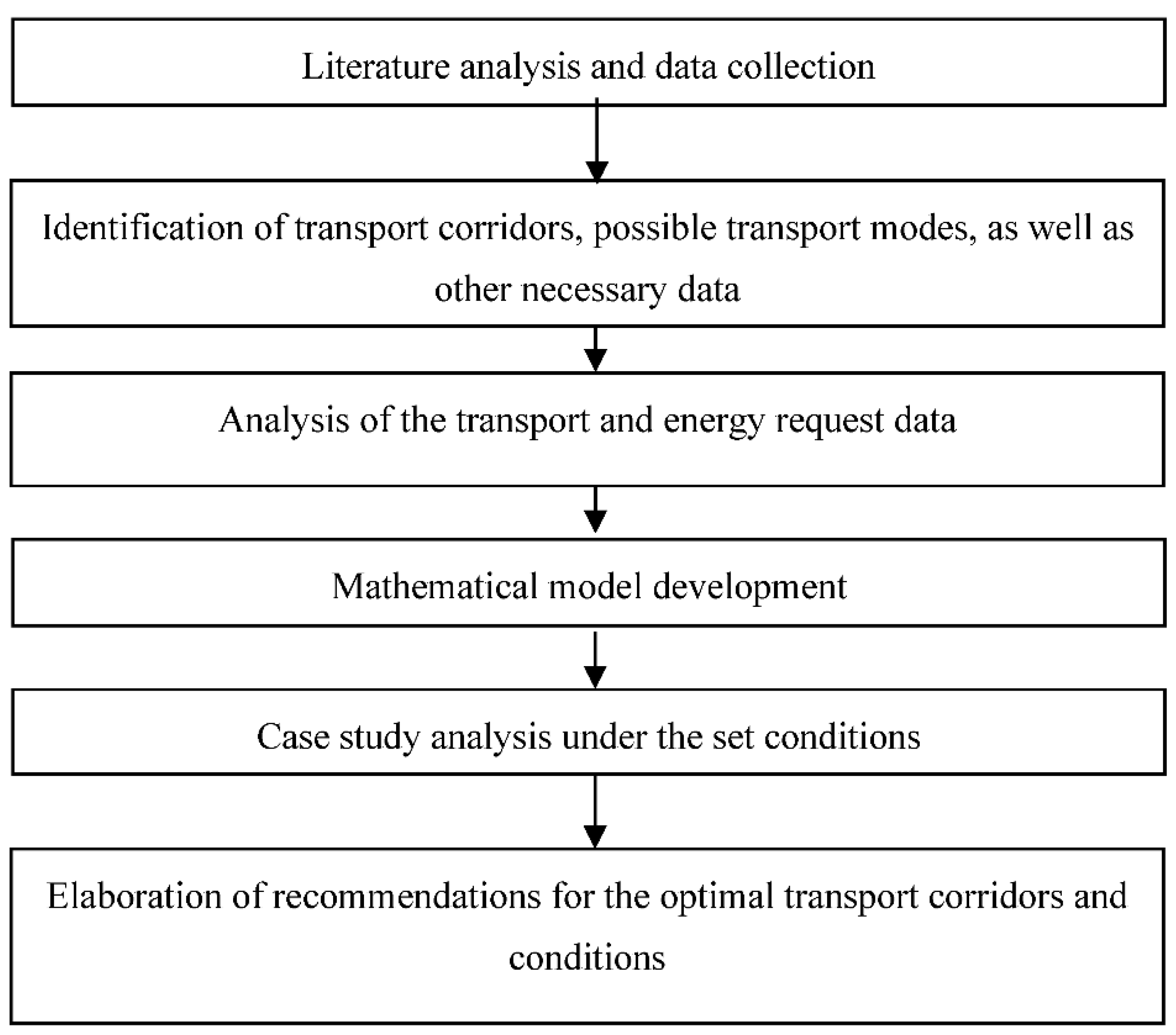
3.1. Research Methodology

To develop the research methodology, an initial study was performed to analyze available literature, which then allowed a review to be conducted of “the state of the art”, in cargo transportation between regions, ports and consignees/shippers, transport corridors selection, including transportation costs, time, energy (fuel) using by transport means, existing models used for the selection optimal transport corridors, etc. Data were collected based on literature sources and observations of cargo transportation between regions, ports and consignees/shippers movement in transport corridors and experimental data received from ports, consignees/shippers, forwarding and transport companies (Figure 1).

The methodology was stated in this research, which considers possible transport corridors, transport means, energy amounts, transportation time, and cost factors. The main cargo transportation parameters were considered, such as: transportation distances between main transportation points and “last mile” distances, transportation costs, fuel consumption on different transportation sections, cargo loading equipment, transport means capacity, fuel consumption by transport modes and cargo handling equipment, transportation and reloading time, transport modes and cargo handling equipment power and usage time, used coefficients, etc. (Figure 1).

Hydro-meteorological and hydrological conditions for the inland waterway ships (barges) sailing were considered in the proposed method, e.g., wind velocity, wind course angle (the angle to a waterway access), current velocity, current course angle to barge, etc.

Moreover, additional data, such as navigation channels (waterways) width and channel depths, which were necessary for conducting the research were collected and analyzed. Furthermore, the relevant coefficients, received by theoretical and experimental investigations, were considered.

A mathematical model was developed to calculate transportation time and costs, fuel consumption and fuel quality, as well as hydro meteorological conditions on inland waterways, roads, railways, and cargo loading points. This model takes into consideration implementation of the following steps:

• Collection and analysis of the data mentioned above.
• Planning possible distances between regions, ports, and main reloading points (intermodal terminals).
• Calculation of the cargo reloading time and costs in cargo reloading points, based on collected data.
• Calculation of particular transportation parameters, such as time costs and fuel consumption.
• Calculations of transport modes energy comparative index for the transport corridors.
• Drawing the conclusions and recommendations for the specific conditions.

The boundary conditions of the methodology and the model are as follows: inland water transport (barges) capacity depends on the infrastructure parameters; minimum cargo flow for the development optimal superstructure; optimal distances between regions, ports and consignees/shippers locations by different transport corridors; minimum possible reloading points on transport corridors for the transportation costs and time minimization; hydro-meteorological conditions that avoid additional costs, such as icebreakers on inland waterways. In cases in which the distance between transport corridors is less than 20% (for road and railway transport), boundary conditions based on possible real reloading conditions are not taken into account, because, for example, the amount of loading equipment and productivity difference it is very low.

The proposed methodology was verified on the basis of case study. The containers transportation between Klaipeda port and Kaunas free economic zone was analyzed in detail, and calculations based on real data were carried out. On the basis of the archived results, recommendations for the selected optimal transport corridors were proposed. At same time, proposed methodology could be adopted in any other similar places and conditions.

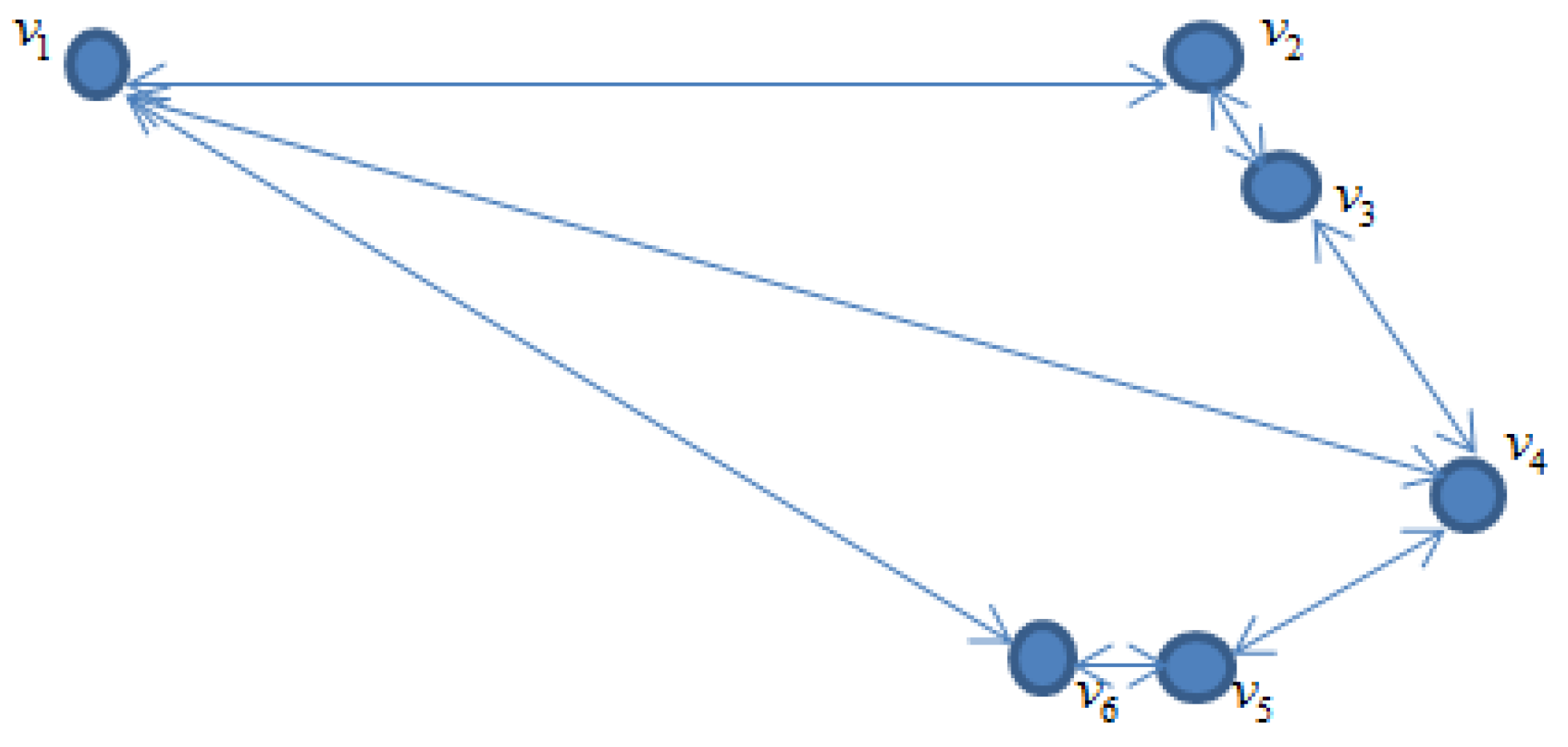
3.2. Mathematical Model

The main conditions for the development of the route network are to estimate possible alternative routes between regions, and or ports and consignee locations, and to create preconditions for optimal route selection, assessing the best technical possibilities, the lowest possible energy consumption and acceptable economic conditions.

A methodology for the cargo transportation optimization between regions, ports and consignee locations was developed on the basis of multi-criteria and comparison analysis. The main tasks of the developed methodology are based on the research on theoretical models, which can assist with finding optimal transportation modes, minimization energy requirements and practically useful applications.

Considering at least one transport mode capacity (the number of containers transporting by train), it is possible to perform an analysis and find optimal solutions. Optimal solutions should include assessment of different transport modes time and the costs of transportation and energy requirements.

The development of a sustainable transport system connecting regions and ports with delivery points is extremely important when analyzing various options for cargo delivery between regions and ports and vice versa. In many cases, the “last mile” problem that occurs when using different transport systems during transportation needs to be resolved. The “Last mile” in supply chain management and transportation planning, as well in this article, is the last leg of a journey comprising the movement of people and goods from a transportation hub or other loading/reloading place; for example, a railway station or inland waterways loading/unloading place, to a final destination. For the optimal development of the transport system, it is essential that it is sustainable in terms of time, cost and energy optimization.

In this way, the function of comparing transports corridors and transport modes transport mode comparative index ($K$) can be expressed as follows:

$$K=f(P,T.E\dots )$$

(1)

where: $P$—transportation price function; $T$—transportation time function; $E$—energy consumption function.

Price function can be expressed via transportation lump sum costs (price on different parts of transportation) and the number transport units used, as follows:

$$P=\frac{1}{{\eta }_i}[(P_T+P_{M1}+0,5\cdot P_{IM})N_{TU1}+(0,5\cdot P_{IM}+P_{M2}+P_F)\cdot N_{TU2}+\dots ]$$

(2)

where: ${\eta }_i$—correlation coefficient, for the transport chain could be between 0.95 and 1.0; $P_T$—terminal price for one unit; $P_{M1}$—first chain part transport mode unit price; $P_{IM}$—intermodal terminal price; $P_{M2}$—second transport mode unit price; $P_F$—unit unloading price in final destination; $N_{TU1}$—number of transport mode units on first chain part; $N_{TU2}$—number of transport mode units on the second chain part; +…—other possible elements, such as emission trading payments and so on. The 0.5 coefficient means there is an intermodal terminal price split in transport chain parts (delivery from port to intermodal terminal and delivery from intermodal terminal to final destination).

The transportation time function ($T$) for a specific quantity of cargo units can be expressed as follows:

$$T=\frac{1}{{\eta }_i}[(T_T+\frac{S_1}{v_{M1}}+0,5\cdot T_{IT})\cdot N_{TU1}+(0,5\cdot T_{IT}+\frac{S_2}{v_{M2}}+T_F)\cdot N_{TU2}+\dots ]$$

(3)

where: $T_T$—transport unit time in port terminal; $S_1$—distance between port terminal and final destination or intermodal terminal; $v_{M1}$—average transport mode speed between original cargo transportation place and final destination place or intermodal terminal; $T_{IT}$—transport unit full operation time in intermodal terminal; $S_2$—distance between intermodal terminal and final destination place; $v_{M2}$—average transport mode speed between intermodal terminal and final destination place; $T_F$—average operation time of one transport unit in final destination place; +…—other possible elements, such as waiting convoy time during oversize cargo transportation, and so on.

Energy consumption function ($E$) for a specific quantity of cargo units can be expressed as follows:

$$E=\frac{1}{{\eta }_i}[(E_T+E_{M1}+0,5\cdot E_{IT})\cdot N_{TU1}+(0,5\cdot E_{IT}+E_{M2}+E_F)\cdot N_{TU2}+\dots ]$$

(4)

where: $E_T$—energy demand in original (port) terminal for the loading/unloading transport unit; $E_{M1}$—energy demand on the first chain part for the transport mode unit (transportation from/to the port to/from the intermodal terminal or inland waterway unloading/loading place or the final destination when using a “door to door” system); $E_{IT}$—energy demand in an intermodal terminal or in inland waterway unloading/loading place for one transport unit (for an intermodal terminal or unloading/loading place operations); $E_{M2}$—energy demand on the second chain part for the transport mode unit (transportation from/to intermodal terminal or inland waterway unloading/loading place to/from final destination); $E_F$—energy demand in final destination for unloading/loading operations; +…— other possible elements, such as additional energy consumption due to additional waiting time, bypass some transportation corridor sections, and so on.

Given the average vehicle engine power during the journey, the driving distance and the average driving speed, the total energy used can be calculated using the following formula:

$$E=N_{TM}\frac{S}{v}$$

(5)

where: $N_{TM}$—average vehicle engine power; $S$—driving distance; $v$—average driving speed.

The amount of energy needed by the terminal equipment can be calculated using the average power of the equipment’s motor and the working time.

Transport requires engines that are powerful enough; for example, sea ships consume a lot of fuel. Ships use a lot of fuel while sailing and use a little less when they are at ports or anchorages, i.e., waiting for access to ports. The amount of fuel consumed by a means of transport is calculated during the voyage or during another period. In general, the engine fuel consumption ($Q_f$) can be calculated as follows [2,16]:

$$Q_f={\displaystyle \underset{0}{\overset{T}{\int }}{k}_f}\cdot q_f\cdot N_{TM}\cdot dt$$

(6)

where: $k_f$ is the coefficient, which depends on the type of engine [2]; $q_f$ is the consumption of fuel for the definite engine (kg/kWh); $N_{TM}$ is the engine’s average power during the working period (kW), which can be calculated using Equation (7):

$$N_{TM}=\frac{{\displaystyle \underset{0}{\overset{t}{\int }}{N}_{TMi}\cdot dt}}{t}$$

(7)

where: $N_{TMi}$—is the instantaneous transport means (equipment) engine power (kW); $t$—is the transport means working time in hours.

In order to find optimal solutions, evaluation methods with weight coefficients could be used. Finally, the transport mode comparative index ($K_i$), could be expressed as follows:

$$K_i=\frac{1}{{\eta }_k}(k_P\cdot \frac{P_i}{P_0}+k_T\cdot \frac{T_i}{T_0}+k_E\cdot \frac{E_i}{E_0}+k_i\frac{A_i}{A_0})$$

(8)

where: ${\eta }_K$—correlation coefficient, for the transport corridors, in case of similar factors; for example, the “last mile” situation for the railway and inland waterway transport modes and so on, could be 0.97–0.99, using more factors could improve the identification of correlation coefficients by using a matrix system [18]; $P_i,T_i,E_i$—costs, time and energy demand for the analyzing transport corridor; $P_0,T_0,E_0$—costs, time and energy demand for the etalon, which can be selected by expert method, transport corridor; $k_P$—weight coefficient of the transport corridor’s costs. Depending on the type of cargo, it could be taken between 0.3–0.4; $k_T$—weight coefficient of the transport corridor’s transportation time. This depends on the type of cargo and could be taken between 0.2–0.3;

$k_E$ is the weight coefficient of the transport corridor’s energy (fuel) demand. It depends on the transportation conditions and areas and could be taken between 0.2–0.3; $k_i,A_i,A_0$—other possible factors and weight coefficients; for example, emissions, cargo weights and other factors, which are important for the transportation cases. The sum of the weighting factors must be equal to one.

Equation (8) is based on multi-criteria methods and can be used for many tasks; for example, for passenger and cargo transportation optimization, including environmental impact evaluation in case only a few transport corridors could be used, as well for the logistics chains evaluations. Using the mentioned equation is necessary to in order to pay attention to weight coefficients, which can be calculated via the matrix in the existing wide data base or could be used expert methods in case of limited real data.

For the optimal transportation way and energy saving, it is necessary to find the best transport network, and this could be achieved using the graph theory method. The application of graph theory method is used, in which the model is built in such a way that incorporates a set of vertices, which represent possible transport roads or corridors, and a set of edges, which represents the main connecting points, such as terminals, railway stations (intermodal terminals) and final destination points. This could be modeled as a graph tree and expressed as follows [41,42,43,44,45]:

$$G=(V,E)$$

(9)

where: $V$—the set of vertices; $E$—the set of edges. Such a graph model can be expressed as shown in Figure 2.

The departure point could be Seaport ($v_1$) or another departure point, and the destination point could be the same as cargo consignee ($v_4$). Depending on the transport mode, it could be a direct delivery by road transport mode (from door to door), which means that from ($v_1$) to ($v_4$), a railway mode could be used between points $v_1$ and $v_2$, from point $v_2$ to point $v_3$, and from point $v_3$ to point $v_4$, road transport could be used as the “last mile destination“. Similarly, an inland water way transport mode could be used from seaport point $v_1$ up to inland waterway ships loading/unloading place $v_5$, and road transport could be used from inland waterway transport loading/unloading place $v_6$ to final destination $v_4$ as the “last mile destination”.

For the graph tree, presented in Figure 2, the sets of vertices and the set of edges can be expressed as follows [41]:

$$V=\left\{v_1,v_2,v_3,v_4,v_5\dots \right\}$$

(10)

$$E=\left\{(v_1,v_2)(v_2,v_3)(v_1,v_3)(v_1,v_4)(v_4,v_3)\dots \right\}$$

(11)

The incident matrix of all vertices, consisting of connecting direct graph connections provided by the graph tree G, can be presented as follows [42]:

$$A=a_{ij},$$

(12)

where

$$a_{ij}=\left\{\begin{array}{l}{1\mathrm{if}v}_i{\mathrm{is}\mathrm{the}\mathrm{initial}\mathrm{vertex}\mathrm{of}e}_j\\ {-1\mathrm{if}v}_i{\mathrm{is}\mathrm{the}\mathrm{terminal}\mathrm{vertex}\mathrm{of}e}_j\\ 0\mathrm{otherwise}.\end{array}\right.$$

In this case, study (Figure 2) for possible transport corridors network adjacency matrix can be explained as follows [41]:

$$A=\left\{\begin{array}{l}{v}_1,v_2,v_3,v_4,\dots \\ v_2\\ v_3\\ v_4\\ \dots \end{array}\right\}$$

(13)

For the graph tree covering the transport corridors network, which is explained in Figure 2, the mentioned matrix in formula (12) can be calculated as follows:

$$A=\left. [\begin{array}{l}0111\dots \\ 1010\\ 1101\\ 1010\\ \dots \end{array}\right]$$

(14)

Matrix (14) could be used for the calculation of time, costs and energy demand. Finally, the optimum distances, optimal price or minimum energy demand in transport routes in the network could be calculated using the following optimization formula [41,42,43]:

$$f:E\Rightarrow R^{+},$$

(15)

It is also necessary to find a graph tree $T=(V{E}^{\prime })$ price, optimal distance or minimum energy demand $F(T)$:,

$$F(T)={\displaystyle \sum _{xy\in E^{\prime }}f(xy)},$$

(16)

where: $f(xy)$—minimum price, optimal distance or minimum energy demand.

Here, the edges $e=xy\in E$ as minimum price, optimal distance or minimum energy demand could be calculated as follows [41]:

$$f(e)=\underset{xy\in E}{\min }f(xy),$$

(17)

Based on the proposed graph theory, it is possible to design optimal transport corridors based on transportation time, cost and energy saving (minimum demand) [44,45].

For the analysis and evaluation of the experimental or collected data distribution, it is proposed to use a dispersion ($\sigma$) [18,20] method to find the possible factors range (band).

$${\sigma }^2=\frac{1}{n-1}{\displaystyle \sum _1^{n-1}{(x_i-x_m)}^2}$$

(18)

Here: $n$—measured quantity (statistics data); $x_i$ measures results; $x_m$—mathematics’ factor, which can be calculated as follows:

$$x_m=\frac{1}{n}{\displaystyle \sum _1^n{x}_i},$$

(19)

Then, the relative transport mode comparative index band ($\mathsf{\Delta }{K}_i$) can be calculated using the following formula:

$$\mathsf{\Delta }{K}_i=\pm \sqrt{{\sigma }^2},$$

(20)

The main scientific contribution of the developed methodology is based on using graph theory, multi-criteria and comparative methods. The received tool is more accurate in comparison with existing methods [3,25,44,45,46] for evaluation of optimal transportation possibilities, including energy demand between regions, ports and consignee locations, for the evaluation.

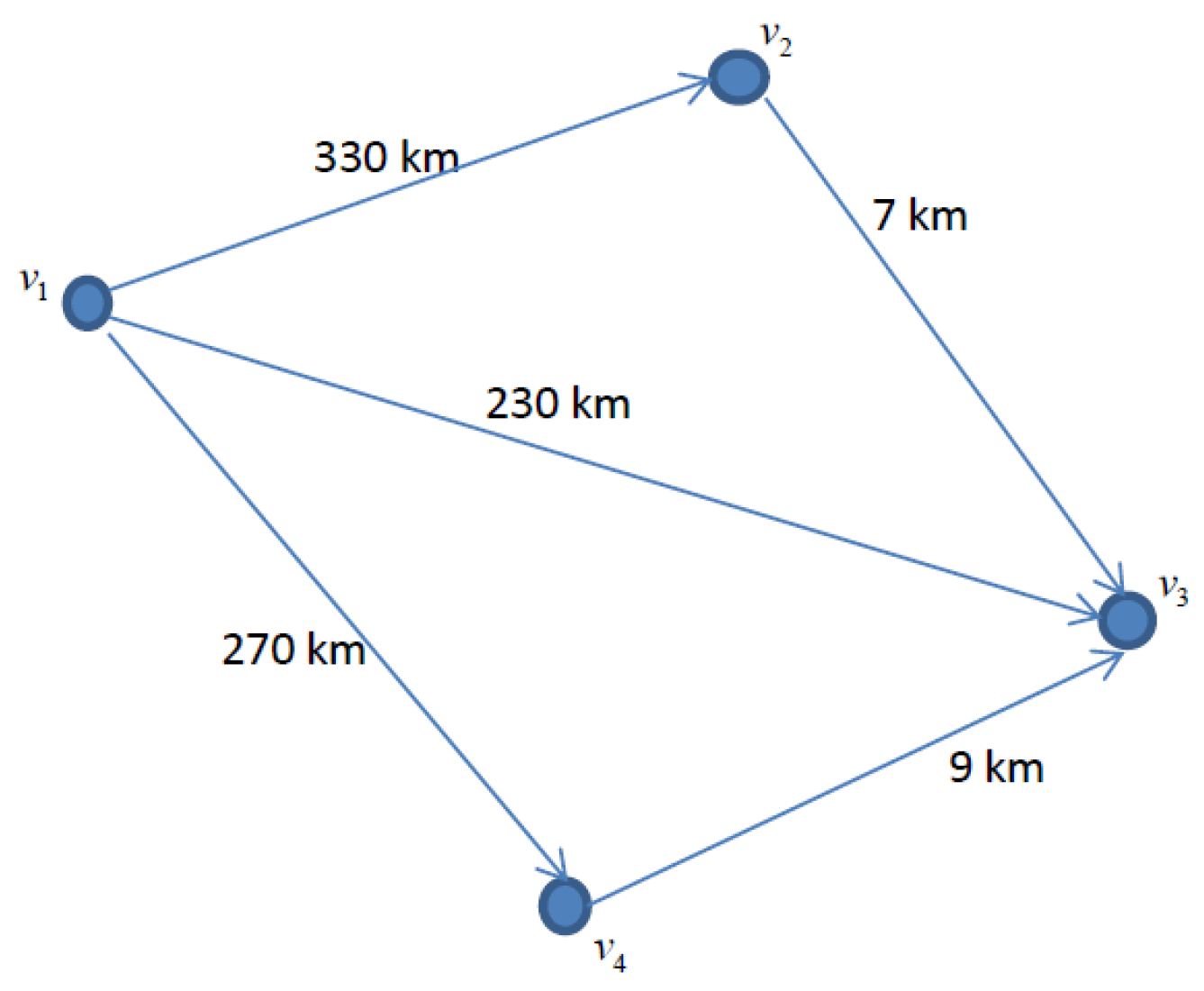
4. Case Study on the Different Transport Modes between Ports and Consignee Location Evaluation (Lithuania Case)

Analysis of cargo transportation and use of methodology, presented in Section 3, were performed as practical tasks—optimization of cargo transportation processes between port and consignee locations. For this case study, transportation of containers from (to) Klaipeda port to (from) Kaunas free economic zone was undertaken. It is possible to use three transport modes between transportation points: road, railway and waterway transport. In case of railway and inland waterway transportation, it is necessary use “last mile” solutions (Figure 3) [27].

Analysis of the modes of transport between Klaipeda port and Kaunas showed that the power of every truck engine is about 300–350 kW (total used engine power is about 15,000 kW), and train locomotive engine power, on average, is about 3000 kW. It is worth noting that, on average, one freight train can replace about 50 trucks [8,20,36,38]. The “Last mile” destination should be organized between the railway station and the destination point. Finally, it is also possible to use an inland waterway transport option between Klaipeda port and the Kaunas area using the Nemunas river, and in this case, the same cargo quantities transportation request one inland waterway ship, which uses an engine with power of about 400 kW [27].

The graph model for the selected transport systems in general between Klaipeda port and Kaunas free economic zone (FEZ) for customers’ transportation situation (distances) can be explained as follows (Figure 4) [41]:

In Figure 4, the distances are as follows: 330 km by railway from Klaipeda container terminal to Kaunas intermodal terminal; 7 km by road transport from Kaunas intermodal terminal to Kaunas free economic zone; 230 km by road transport from Klaipeda container terminal to Kaunas FEZ free economic zone; 270 km by inland waterway from Klaipeda container terminal to inland waterways loading/unloading place in the Kaunas area; and 9 km by road transport from the inland waterway barges loading place in Kaunas area to Kaunas FEZ free economic zone.

A typical transportation case in Lithuania, based on data received during analysis, considers a train, includes a propelled barge, which can transport about 80 TEU (Figure 5). For some 20′ (TEU—Twenty Foot Equivalent Unit) and 40′ foot or 2 TEU containers, it will be necessary to have approximately 50 road transport trucks. Propelled barge engine power is about 400 kW, and the average speed is about 15 km/h (barges work on Lithuania inland water ways). The engine power of a train locomotive, which can transport 80 TEU, is about 4000 kW, and the average speed is about 35 km/h (in this case, according to our investigations, the average power of a train locomotive is about 3000 kW). The engine power of one road truck is about 300 kW, and the average speed is about 60 km/h [5,7,8,23]. The abovementioned transport modes parameters should be taken as a basis for the calculation of transportation time, costs and energy demand using the methodology described in Section 3 of this paper. It is also necessary to take distribution procedures at intermodal terminal into account in cases in which railway transport and road transport on “last mile” is to be used. The latter shall also apply in cases in which waterway transport and road transport on the “last mile” are used.

The adjacency matrix for the transportation distances at Figure 4 could be made as follows:

$$A_D=\left. [\begin{array}{cccc}0& 330& 230& 270\\ 330& 0& 7& 0\\ 230& 7& 0& 9\\ 270& 0& 9& 0\end{array}\right]$$

Inland waterway barges carry a lot of cargo with a relatively low-power engine, and may keep a constant speed in case of the absence of any locks or other obstacles on the waterway. At the same time, due to required transhipment between inland waterways (railways) transport mode and road transport, the following items need to be considered: “last mile” distance, additional time, costs. Energy demand and other items, such as environmental impact [46,47,48,49]. Transport modes and transhipment points during transportation process between the seaport and final cargo destination are presented in Figure 6.

Transhipment at the intermodal terminal or at the inland waterway barges loading and storage site by a mobile crane with 15 movements per hour and average engine power of about 500 kW should be considered when calculating the total transport time, costs and energy demand.

The adjacency matrix of the graph at Figure 6 for the transportation time in hours in case of transportation of 80 TEU (on average, delivery of 50 boxes using one train or one barge, or 50 road trucks), taking into account the conditions mentioned above, could be made as follows:

$$A_T=\left. [\begin{array}{cccccc}0& 9& 12& 37& 0& 0\\ 9& 0& 3& 28& 0& 0\\ 12& 3& 0& 25& 0& 0\\ 150& 28& 25& 0& 25& 28\\ 21& 0& 0& 25& 0& 3\\ 18& 0& 0& 28& 3& 0\end{array}\right]$$

Using the dispersion method (Formulas (17)–(19)), experiments on the real transportation time have shown that differences in the road transport reach up to 7–8%, mainly due to traffic conditions in city areas. Differences in railway transport reach up to 5–7% in the event of good planning, and differences in inland waterway transport can reach up to 10%, mainly due to departure issues from the port area.

The adjacency matrix of the graph at Figure 6 for the transportation costs in EUR in case of transportation of 80 TEU (on average, delivery of 50 boxes using one train or one barge, or 50 road trucks), could be made as follows:

$$A_P=\left. [\begin{array}{cccccc}0& 4000& 6500& 9000& 0& 0\\ 4000& 0& 2500& 5000& 0& 0\\ 6500& 2500& 0& 2500& 0& 0\\ \mathrm{12,500}& 5000& 2500& 0& 2500& 5000\\ 7500& 0& 0& 2500& 0& 2500\\ 5000& 0& 0& 5000& 2500& 0\end{array}\right]$$

The adjacency matrix of the graph in Figure 6 for the total engines power in kW (on average, delivery of 50 boxes using one train or one barge, or 50 road trucks), could be made as follows:

$$A_N=\left. [\begin{array}{cccccc}0& 2500& 250& 200& 0& 0\\ 2500& 0& 250& 200& 0& 0\\ 2750& 250& 0& 200& 0& 0\\ 200& 350& 200& 0& 200& 450\\ 600& 0& 0& 200& 0& 250\\ 400& 0& 0& 450& 250& 0\end{array}\right]$$

The adjacency matrix of the graph in Figure 6 for the fuel consumption in kg (on average, delivery of 50 boxes using one train or one barge, or 50 road trucks) for transportation of 80 TEU could be made as follows:

$$A_K=\left. [\begin{array}{cccccc}0& 3600& 3720& 4320& 0& 0\\ 3600& 0& 120& 720& 0& 0\\ 3720& 120& 0& 600& 0& 0\\ 4800& 720& 600& 0& 600& 720\\ 1200& 0& 0& 600& 0& 120\\ 1080& 0& 0& 720& 120& 0\end{array}\right]$$

Presented in this section, the adjacency matrix, sometimes called the connection matrix, of a simple labeled graph is a matrix with rows and columns labeled by graph vertices. For a simple graph with no self-loops, the adjacency matrix must have zero on the diagonal.

The solution of the presented adjacency matrices for a specific transport corridor or a specific type of transport is carried out by adapting them to specific conditions and applying standard solutions of such a matrix [41,43]. The comparative results of the solutions of the indicated matrixes in this section are presented in Figure 7.

Experiments on the real fuel consumption in analyzed transport corridors have shown that differences in the road transport reach up to 5–12%, mainly due to traffic conditions; differences in railway transport reach up to 6–11% in case of good planning and differences in inland waterway transport reach up to 10%, mainly due to maneuvering of the ship.

Transportation of 80 TEU between the Klaipeda port container terminal and Kaunas FEZ free economic zone (on average, 50 containers (boxes)) uses one train or one barge, or 50 road trucks between port container terminals and Kaunas FEZ free economic zone or 50 road trucks (voyage) for the “last mile” destination between the intermodal terminal or inland waterway cargo loading place and the Kaunas FEZ free economic zone. This means that road transport can deliver cargo “door-to-door”.

Rail transport can deliver cargo from the port to Kaunas intermodal terminal. After that, cargo from the intermodal terminal to Kaunas FEZ Free Economic Zone can be transported by road via “last mile” transportation.

Inland waterway transport can be used for the containers from the port of Klaipeda to the place of unloading of inland waterway cargo (Kaunas). After that (cargo loading place in inland waterways), the cargo is transported by road from the place of unloading to the Kaunas FEZ Free Economic Zone by road transport for the “last mile”.

Transport modes today mainly use diesel fuel. Meanwhile, some transport modes start use LNG fuel, which has about 15 percent higher energy capacity and is more environmentally friendly.

The analysis of differences in the comparative index ($K_i$) of transport types using Equation (8), based on the theoretical and experimental research results presented in this paper, for transportation between the Klaipeda container terminal and the Kaunas FEZ and using the methodology, is presented in Section 3. Equation (8) for the selected conditions can be written as follows:

$$K_i=\frac{1}{{\eta }_k}(k_P\cdot \frac{P_i}{P_0}+k_T\cdot \frac{T_i}{T_0}+k_E\cdot \frac{E_i}{E_0})$$

where the weighting factor of transportation costs is taken as 0.5, the weighting factor of transportation time is 0.3, and the energy consumption factor is 0.2. The correlation coefficient is 0.98 (correlation mainly exist in transportation conditions between rail and inland waterway transport).

Using diesel and LNG fuel and evaluating the transportation scheme and adjacency matrices shown in Figure 6, the results of the comparative index ($K_i$) calculation of transport modes are presented in Figure 7.

The received transport mode energy comparative index shows that containers transportation between the selected container terminal and destination in the free economic zone is more useful for railway or inland waterway transport, including the “last mile” destination.

Relative ($\mathsf{\Delta }{K}_i$) is assessed for the selected case study by assessing the cost of transportation, time and fuel consumption, using the real parameters presented in

Table 3. Relative ($\mathsf{\Delta }{K}_i$) for the selected case study based on collected real data.

Transport Mode	Number of Real Data (Cases)	$\mathbf{Relative}\left({\mathit{K}}_{\mathit{i}}\right)$	Dispersion	$\pm \mathsf{\Delta }{\mathit{K}}_{\mathit{i}}$
Road	53	1.0	0.034	0.18
Railway	22	0.65	0.021	0.14
Inland waterway	7	0.53	0.012	0.11

.

The obtained results indicate that container transportation between Klaipeda port container terminal and Kaunas FEZ Free Economic Zone is the most acceptable using water or railway transport (difference in relative ($\mathsf{\Delta }{K}_i$) is up to 35–47%).

At the same time, it is necessary to take into account that if containers must be delivered in the shortest possible time, road transport for the direct transportation between regions, ports terminals and cargo recipients/shippers could be used as well.

5. Discussions

Developing a theoretical methodology and application for the transportation optimization that seeks to optimize transportation processes and decrease the amount of energy consumed between the port and cargo receiver/sender oriented on practical matters often requires a quantitative technological approach that includes factors from economics and energy demand [50,51,52]. Optimal transport corridor selection and its effectiveness is recommended as a benchmark to reflect the operating conditions of the selected transport corridors and/or transport modes due to disruption [53]. The results of the scientific literature review of related literature sources, related to similar tasks [54,55,56], indicated that a developed methodology of the transportation parameters evaluation is useful for the practical tasks and could be useful in many similar transportation cases. However, weight coefficients, which are used in developed methodology, could be discussed and further investigated. In some regions, there are different regulations; for example, the permitted weight of the cargo, size parameters and other requirements are different, and it is necessary to adopt these for real conditions. Therefore, we try to relate productivity benchmarks based on a comparative index for transportation using different transport modes management’s risks and quantitative transportation time, costs, and an environmental impact analysis approach.

Carrying out real transportation experiments on the routes indicated in the paper, as well as theoretical calculations using the methodology developed in this paper, showed the practical importance of optimization of transportation processes, as there are no big differences between the results (the experimental and theoretical calculations results’ differences mainly were up to 10–12%). The specified methodology for optimization of transportation processes, integrated assessments using the approach set out in the paper has attracted a great deal of interest from logistics and transport companies.

During the experiments, the transport companies, as well as the authors of the paper, identified some additional sources of uncertainty that could be useful for future research. This is mainly due to additional disruptions on individual routes, such as traffic congestion on roads, especially ice on roads during the winter. Weighting factors for the comparative method, adapted to the specific routes and conditions, are very important for future research.

In future research, it is also necessary to pay attention to the constraints of the economic market; fluctuations in demand, risks, levels of fuel prices and prices practiced in the other markets, customs regulations, international politics, insurance, environmental factors and macroeconomics.

To reduce uncertainty and errors, several recommendations are provided, which include more flexible communication between the parts of the logistics chain between the port and the consignees/shippers, prompting an exchange of information and quick response to possible changes.

Analysis of the existing methods and comparison with the proposed development method, as well as future research, is presented on

Table 4. Differences between existing transportation evaluation methods, developed method in this paper and future research prospects.

Factors	Existing Methods	Developed Method in This Paper	Future Research Prospects
Transportation time, costs and energy demand factors	Exist methods evaluate costs and time transportation; problematic to evaluate energy demand	It is possible evaluate optimal costs, transportation time, energy demand and additional factors	It is important make research works that more accurate receive factors weight coefficients
Environmental factors	It is possible to evaluate environmental impact factors and existing limitations and provide complex evaluation together with costs, time and energy demand evaluation	Method could be adopted evaluate economics and environmental factors	In future need research works more accurate evaluate economics and environmental factors in case of non-standard transportation processes
Complex evaluation of the main factors	Problematic, because in case of many factors not clear systems	Possible, but need clear evaluate weight of the factors	Finding weight of the factors could be main research tasks in future adopted to concrete conditions

.

Studies have shown that the approach to optimizing transportation and reducing energy demand presented in the paper can be adapted to other regions where similar conditions exist.

In this study, we have found that several parameters are needed that can be quantified and that are consistent with the management of transport corridors and transport modes by optimizing transport processes and energy demand. The transport mode comparative index ($K_i$) used in this paper includes economic, time and energy demand factors. This allows the impact category to be assessed in the selected transport corridor. The three main or more factors can then be used as the basis for stakeholders to plan or improve the organization of the transportation process. Based on the results of the study, it has been found that, at least for the time being, the price factor in the study case is the most important, and has the greatest influence on the choice of transport corridor and vehicles.

6. Conclusions

Possible transport alternative routes between ports and consignors/consignees using different modes of transport have been explored, which is very important in light of the demanding economic situation and energy demand requirements.

The use of the graph theory method for the optimization of shipments between ports and consignors/consignees using different modes of transport is important from a theoretical and practical point of view, and has aroused great interest among transport researchers and transport and logistics companies.

The developed ($K_i$) evaluation model presented in the paper allows us to determine the optimal transportation options, considering the transportation time, price and energy demand factors.

The analysis of the case using the developed methodology and real experimental factors of transportation cost, time and energy demand confirmed the theoretical expediency and practical applicability of the developed methodology.

The results of the case study have shown that the developed methodology can be successfully applied in many parts of the world.

Green transportation solutions are also very important because terminals and industry regions are located close to living areas, and it is necessary to reduce the energy demand and environmental impact of transport and increase living standards in these areas.

The proposed calculation of the transport mode comparative index can assist the transport and industry companies, as well as administrations, with identification of the most optimal solutions in transport infrastructure development and choice of optimal transport corridors and transport modes.

“Last mile” logistics are very important in multimodal and intermodal transport. Optimal solutions for this part of transportation require research and adaptation to specific locations, such as industrial and densely populated areas.

Combining different transport modes can optimize transport links, transportation costs, minimize transportation time and decrease energy demand.

References

1. Ritchie, H.; Roser, M.; Rosado, P. Energy. 2020. Available online: https://ourworldindata.org/energy (accessed on 15 May 2022).
2. U.S. Department of Energy Washington. Global Transportation Energy Consumption: Examination of Scenarios to 2040 Using ITEDD; U.S. Department of Energy Washington: Washington, DC, USA, 2017; 38p.
3. Kwon, M.; Lee, J.; Hong, Y.S. Product-service system business modelling methodology using morphological analysis. Sustainability 2020, 11, 1376. [Google Scholar] [CrossRef] [Green Version]
4. Szeto, W.Y.; Lo, H.K. Transportation Network Improvement and Tolling Strategies: The Issue of Intergeneration Equity. Transp. Res. Part A Policy Pract. 2006, 40, 227–243. [Google Scholar] [CrossRef]
5. Jarašūnienė, A.; Čižiūnienė, K.; Petraška, A. Research on rail and maritime transport interoperability in the area of information systems: The case of Lithuania. Transport 2019, 34, 467–475. [Google Scholar] [CrossRef] [Green Version]
6. Zhou, W.; You, X.; Fan, W. A mixed integer linear programming method for simultaneous multi-periodic train timetabling and routing on a high-speed rail network. Sustainability 2020, 12, 1131. [Google Scholar] [CrossRef] [Green Version]
7. Saakian, I.; Savchuk, V. Railway transportation: Problems and solutions. Probl. Econ. Transit. 2013, 56, 73–95. [Google Scholar] [CrossRef]
8. Mańkowska, M. The competitiveness of cross-border transportation networks: A case study of the Szczecin–Berlin inland waterway. Sci. J. Zesz. Nauk. Marit. Univ. Szczec. 2019, 58, 93–104. [Google Scholar] [CrossRef]
9. Valkhof, H.H.; Hoogeveen, T.; Dallinga, R.P.; Toxopeus, L.S. A Tug and Barge System for Sea and River Service. SNAME Annu. Meet. 2000, 24. Available online: https://www.researchgate.net/publication/257817071_A_Tug_and_barge_system_for_sea_and_river_service (accessed on 15 May 2022).
10. Müller, J.; Straub, M.; Richter, G.; Rudloff, C. Integration of Different Mobility Behaviors and Intermodal Trips in MATSim. Sustainability 2022, 14, 428. [Google Scholar] [CrossRef]
11. Bouman, E.A.; Lindstad, E.; Rialland, A.I.; Strømman, A.H. State-of-the-art technologies, measures, and potential for reducing GHG emissions from shipping–A review. Transp. Res. Part D Transp. Environ. 2017, 52, 408–421. [Google Scholar] [CrossRef]
12. Ali, N.; Nakayama, S.; Yamaguchi, H. Analysis of Bus Fare Structure to Observe Modal Shift, Operator Profit, and Land-Use Choices through Combined Unified Transport Model. Sustainability 2022, 14, 139. [Google Scholar] [CrossRef]
13. Smaoui, H.; Zouhri, L.; Kaidi, S. Identification of Hydrodynamic Dispersion Tensor by Optimization Algorithm Based LBM/CMA-ES Combination. Water 2022, 14, 125. [Google Scholar] [CrossRef]
14. Di Vaio, A.; Varriale, L. Management innovation for environmental sustainability in seaports: Managerial accounting instruments and training for competitive green ports beyond the regulations. Sustainability 2018, 10, 783. [Google Scholar] [CrossRef] [Green Version]
15. Hale, J.; Long, S.A. Time Series Sustainability Assessment of a Partial Energy Portfolio Transition. Energies 2021, 14, 141. [Google Scholar] [CrossRef]
16. Paulauskas, V.; Filina-Dawidowicz, L.; Paulauskas, D. The Method to Decrease Emissions from Ships in Port Areas. Sustainability 2020, 12, 4374. [Google Scholar] [CrossRef]
17. Colette, A.; Granier, C.Ø.; Hodnebrog, Ø.H.; Jakobs, H.; Maurizi, A.; Nyiri, A.; Bessagnet, B.; D’Angiola, A.; D’Isidoro, M.; Gauss, M. Air quality trends in Europe over the past decade: A first multi-model assessment. Atmos. Chem. Phys. 2011, 11, 11657–11678. [Google Scholar] [CrossRef] [Green Version]
18. Semenov, I.N.; Filina-Dawidowicz, L. Topology-based Approach to the Modernization of Transport and Logistics Systems with Hybrid Architecture. Part 1 Proof—Concept Study. Arch. Transp. 2019, 43, 105–124. [Google Scholar]
19. Ignatavicius, G.; Toleikiene, M. Optimization of the conservation of rare and vulnerable plant species in the perspective of climate change in Lithuanian (nature) reserves. Arch. Environ. Prot. 2017, 43, 61–73. [Google Scholar] [CrossRef] [Green Version]
20. Paulauskas, V. Ships Entering the Ports; N.I.M.S Publish House: Riga, Latvia, 2013; 240p, ISBN 9984-679-71-3. [Google Scholar]
21. Omarov, M.; Ismail, S.; Rani, W.N.M.W.M.; Durdyev, S. Estimation of Traffic Delay Due to U-Turns at Uncontrolled Medians: Case Study in Phnom Penh, Cambodia. Sustainability 2022, 14, 118. [Google Scholar] [CrossRef]
22. Penmetsa, P.; Ghosh, I.; Chandra, S. Evaluation of performance measures for two-lane intercity highways under mixed traffic conditions. J. Transp. Eng. 2015, 141, 04015021. [Google Scholar] [CrossRef]
23. Romanovaa, A.; Vygnanova, A.; Vygnanovaa, M.; Sokolovaa, E.; Eiduks, J. Problems of the formation of a single transport space on sections of international transport corridors. ICTE Transp. Logistics. 2019, 149, 537–541. [Google Scholar] [CrossRef]
24. Belen, M.; Emilio Ortega, E.; Cuevas-Wizner, R.; Ledda, A.; Andrea De Montis, A. Assessing road network resilience: An accessibility comparative analysis. Transp. Res. Part D 2021, 95, 102851. [Google Scholar] [CrossRef]
25. Li, Y.; Chen, Y. Driver Vision Based Perception-Response Time Prediction and Assistance Model on Mountain Highway Curve. Int. J. Environ. Res. Public Health 2017, 14, 31. [Google Scholar] [CrossRef]
26. Hu, Q.; Gu, W.; Wang, S. Optimal subsidy scheme design for promoting intermodal freight transport. Transp. Res. Part E 2021, 157, 102561. [Google Scholar] [CrossRef]
27. Lithuania Transport Map. 2022. Available online: https://www.vle.lt/straipsnis/lietuvos-transportas/ (accessed on 15 May 2022).
28. Jezierski, W.; Sadowska, B.; Pawłowski, K. Impact of Changes in the Required Thermal Insulation of Building Envelope on Energy Demand, Heating Costs, Emissions, and Temperature in Buildings. Energies 2021, 14, 56. [Google Scholar] [CrossRef]
29. Šakalys, R.; Batarlienė, N. Research on intermodal terminal interaction in international transport corridors. Procedia Eng. 2017, 187, 281–288. [Google Scholar] [CrossRef]
30. European Inland Waterways Map. Available online: https://unece.org/DAM/trans/main/sc3/AGN_map_2018.pdf (accessed on 15 May 2022).
31. Ypsilantis, P.; Zuidwijk, R. Collaborative fleet deployment and routing for sustainable transport. Sustainablitiy 2019, 11, 5666. [Google Scholar] [CrossRef] [Green Version]
32. Kotug Forms Inland Shipping Division Based on Electric Pusher Tugs. 2021. Available online: https://www.offshore-energy.biz/kotug-forms-inland-shipping-division-based-on-electric-pusher-tugs/ (accessed on 15 May 2022).
33. Łebkowski, A. Reduction of fuel consumption and pollution emissions in inland water transport by application of hybrid powertrain. Energies 2018, 11, 1981. [Google Scholar] [CrossRef] [Green Version]
34. Hendrickx, C.; Breemersch, T. The Effect of Climate Change on Inland Waterway Transport. Procedia—Soc. Behav. Sci. 2012, 48, 1837–1847. [Google Scholar] [CrossRef] [Green Version]
35. Translate File: Freight Transport in the EU-28 Modal Split of Inland Transport Modes (% of Total Tonne-Kilometres). 2017. Available online: https://ec.europa.eu/eurostat/statistics-explained/index.php?title=File:Freight_transport_in_the_EU-28_modal_split_of_inland_transport_modes_(%25_of_total_tonne-kilometres).png&oldid=336869 (accessed on 15 May 2022).
36. Wiegmans, B.; Konings, R. Intermodal Inland Waterway Transport: Modelling Conditions Influencing Its Cost Competitiveness. Asian J. Shipp. Logist. 2015, 31, 273–294. [Google Scholar] [CrossRef] [Green Version]
37. Kurtulus, E.; Cetin, I.B. Assessing the environmental benefits of dry port usage: A case of inland container transport in Turkey. Sustainability 2019, 11, 6793. [Google Scholar] [CrossRef] [Green Version]
38. Inland Waterways Freight Transport by Type of Vessel. 2018. Available online: https://ec.europa.eu/eurostat/statistics-explained (accessed on 10 March 2022).
39. Mako, P.; Dávid, A.; Böhm, P.; Savu, S. Sustainable transport in the Danube region. Sustainability 2021, 13, 6797. [Google Scholar] [CrossRef]
40. Morales-Fusco, P.; Grau, M.; Saurí, S. Effects of RoPax shipping line strategies on freight price and transporter‘s choice. Policy implications for promoting MoS. Transp. Policy 2018, 67, 67–76. [Google Scholar] [CrossRef]
41. Matuliauskas, K. Grafų Teorija; Vilnius University Publish House: Vilnius, Lithuania, 2010; 21p. [Google Scholar]
42. Andreae, T. On independent cycles and edges in graphs. Discrete Math. 1996, 149, 291–297. [Google Scholar] [CrossRef] [Green Version]
43. Bondy, J.A.; Chvatal, V. A method in graph theory. Discret. Math. 1976, 15, 111–135. [Google Scholar] [CrossRef] [Green Version]
44. Curtis, A.R.; Izurieta, C.; Joeris, B.; Lundberg, S.; McConnell, R.M. An Implicit Representation of Chordal Comparability Graphs in Linear Time. The 32nd International Conference on Graph-2006. Theoretic Concepts in Computer Science, LNCS. 2010, Volume 4271, pp. 168–178. Available online: https://www.sciencedirect.com/science/article/pii/S0166218X1000017X (accessed on 15 May 2022). [CrossRef] [Green Version]
45. Fujita, S. Recent results on disjoint cycles in graphs. Electron. Notes Discret. Math. 2005, 22, 409–412. [Google Scholar] [CrossRef]
46. Sadeghian, P.; Hakansson, J.; Zhao, X. Review and evaluation of methods in transport mode detection based on GPS tracking data. Traffic Transp. Eng. 2021, 167–182. [Google Scholar] [CrossRef]
47. Mouschoutzi, M.; Ponis, S.T. A comprehensive literature review on spare parts logistics management in the maritime industry. Shipp. Logist. 2022, 38, 71–83. [Google Scholar] [CrossRef]
48. Gao, S.; Liu, N. Improving the Resilience of Port–Hinterland Container Logistics Transportation Systems: A Bi-Level Programming Approach. Sustainability 2022, 14, 180. [Google Scholar] [CrossRef]
49. Martins, V.; Correia, C.; Cunha-Lopes, I.; Faria, T.; Diapouli, E.; Manousakas, M.I.; Eleftheriadis, K.; Almeida, S.M. Chemical characterisation of particulate matter in urban transport modes. Environ. Sci. 2021, 100, 51–61. [Google Scholar] [CrossRef]
50. Eyring, V.; Köhler, H.W.; Lauer, A.; Lemper, B. Emissions from international shipping. Impact of future technologies on scenarios until 2050. J. Geophys. Res. 2005, 110, D17306. [Google Scholar] [CrossRef]
51. Heinrich, L.; Koschinsky, A.; Markus, T.; Singh, P. Quantifying the fuel consumption, greenhouse gas emissions and air pollution of a potential commercial manganese nodule mining operation. Marit. Policy 2020, 114, 103678. [Google Scholar] [CrossRef]
52. Czermański, E.; Pawłowska, B.; Oniszczuk-Jastrząbek, A.; Cirella, G.T. Decarbonization of maritime transport: Analysis of external costs. Front. Energy Res. 2020, 8, 28. [Google Scholar] [CrossRef] [Green Version]
53. Behdani, B.; Fan, Y.; Wiegmans, B.; Zuidwijk, R. Multimodal Schedule Design for Synchromodal Freight Transport Systems. Eur. J. Transp. Infrastruct. Res. 2016, 16, 424–444. [Google Scholar] [CrossRef] [Green Version]
54. Iheonu, N.O.; Inyama, S.C. On the Optimization of Transportation Problem. Br. J. Math. Comput. Sci. 2016, 13, 1–11. [Google Scholar] [CrossRef]
55. Castaneda, J.; Ghorbani, E.; Ammouriova, M.; Panadero, J.; Juan, A.A. Optimizing Transport Logistics under Uncertainty with Simheuristics: Concepts, Review and Trends. Logistics 2022, 6, 42. [Google Scholar] [CrossRef]
56. Congli, H.; Yixiang, Y. Optimization on Combination of Transport Routes and Modes on Dynamic Programming for a Container Multimodal Transport System. Procedia Eng. 2016, 137, 382–390. [Google Scholar] [CrossRef]
Figure 1. The algorithm of the research methodology.
Applsci 12 10652 g001
Figure 2. The graph tree for transport modes possible ways: v 1 —departure point; v 2 , , v 3 , v 5 , v 6 —waypoints; v 4 —destination point.
Applsci 12 10652 g002
Figure 3. Road, railway and inland waterway transport system between Klaipeda port and Kaunas free economic zone (https://www.vle.lt/straipsnis/lietuvos-transportas/, accessed on 3 September 2022) [27].
Applsci 12 10652 g003
Figure 4. Case study graph: v 1 —Klaipeda container terminal; v 2 —Kaunas intermodal terminal; v 3 —Kaunas free economic zone; v 4 —inland waterway loading place.
Applsci 12 10652 g004
Figure 5. About 80 TEU can be transported by inland waterway transport mode (barge).
Applsci 12 10652 g005
Figure 6. Transport modes and transhipment points adapted in the case study.
Applsci 12 10652 g006
Figure 7. Transport mode energy comparative index (K) for the transportation of 80 TEU between Klaipeda container terminal and Kaunas FEZ free economic zone by different transport roads using diesel and LNG fuels.
Applsci 12 10652 g007