Abstract
Multiples can cause artifacts in imaging; however, they contain information about underground structures. If the internal multiples are removed as a noise, the information contained by the internal multiple will also be removed. This will cause loss of some useful structures in the image. If the multiples and the primary can be separated from the recorded seismic data for imaging, the information contained by the multiples can be used and the artifacts can be attenuated. Here we developed a method to separate the primary and internal multiples and use them in least squares reverse time migration (LSRTM). This method first separates the primary and the internal multiples in the data residual and predicts the wavefield of the primary and internal multiples in a forward- propagated wavefield. We use the high-order Born modeling method to predict the internal multiples. In this method, the internal multiples can be achieved by forward modeling of three times in the time domain. In the internal multiple prediction process, we get the wavefield of the primary and internal multiples in the forward-propagated wavefield. Then, by introducing the weighting matrix, we established the objective function for imaging of the primary and the internal multiples separately. In the calculation of gradient, we use the correlation of primary in the forward-propagated wavefield with the backward-propagated wavefield of the primary in the data residual, and internal multiples in the forward-propagated with the backward-propagated wavefield of internal multiples in the data residual. In this method, the multiple prediction process provided the internal multiples to suppress the artifacts, and LSRTM constructed the model for the multiple prediction process. Finally, we performed numerical tests using synthetic data, and the results indicated that the LSRTM without the internal multiple can suppress not only the artifacts of internal multiples but also some useful structures below the salt dome. LSRTM with primary and internal multiples can suppress the artifact of internal multiples, and the useful structures below the salt dome are compensated in the image.
1. Introduction
In seismic data, there are the primary and multiples. In most cases, the multiples cause artifacts in imaging. Thus, multiple removal methods are an important part of seismic imaging. However, multiples contain information about the subsurface structure, and the imaging of multiples can be a good complement to imaging. As a result, much research has focused on using multiples in imaging.
To reduce the artifacts caused by multiples in imaging, many multiple removal methods have been proposed. Previously, multiple removal methods used the difference in periodicity and travel time between the primary and multiple waves; these methods included the normal moveout (NMO) method, common midpoint stack, Wiener filtering, predictive deconvolution, f-k filter, and Radon transformation [1,2,3,4,5,6,7,8]. Currently, the main internal multiple suppressing methods are based on the wave equation. There are two effectively multiple removal methods that have been widely used. Internal multiple elimination (IME) methods predict internal multiples based on convolution and correlation [9,10,11,12,13]. This method isn’t rely on the model and predicts internal multiples layer-by-layer. The inverse scattering series (ISS) internal multiple attenuation methods is derived from the Lippmann–Schwinger equation [14,15,16,17,18,19,20,21,22]. By computing the component which satisfied the depth condition of its third term in the wavenumber domain, the internal multiples can be predicted. The ISS can predict the multiple precisely but need several Fourier transforms which make its computational cost high. In addition, many other methods have been proposed in recent years. Pica published a model-driven method in 2008 which predicts the internal multiples by using several extrapolations of the data [23]. Marchenko multiple elimination is derived from the coupled Marchenko equation and it is a model independent [24]. It can estimate the surface multiple and internal multiple, and use them in imaging at the same time, but it needs to be improved in complex structure. Berkhout proposed a method called full wave migration (FWM) [25,26,27] which uses one-way wave equation to estimate the primary, surface multiples and internal multiples and uses them in imaging.
Reverse time migration (RTM) was proposed by Whitmore and developed thereafter [28,29,30,31,32]. Least squares migration (LSM) was first proposed by Tarantola in 1984 [33]. Dai et al. [34] proposed LSRTM by combining LSM and RTM in 2011. LSRTM is a method of obtaining the underground reflectivity distribution by solving the optimization problem. LSRTM therefore has more balanced amplitude and less crosstalk than RTM.
Many studies have been proposed to remove multiples or use the multiples as useful information in LSRTM. He and Schuster used both primaries and multiples to image in LSM [35]. Liu et al. proposed the RTM of multiples (RTMM) method in 2011 [36,37]. By cross-correlating the backward-propagated and forward-propagated recorded data on the surface, RTMM can realize the image of the primary and free-surface multiples. Zhang and Schuster proposed the LSRTM of multiples (LSRTMM) method based on RTMM in 2014 [38] to make the amplitude more balanced and to have crosstalk artifacts than RTMM. There are also applications in vertical seismic profile (VSP) ghosts and the viscoacoustic media of LSRTMM [39,40]. Joint LSRTM (JLSRTM) was proposed by Wong et al. in 2015 [41]. Through constructing a modified modeling generator, JLSRTM can jointly image the primary and free-surface multiples and increase the illumination of a complex structure and reduce the artifacts. Liu et al. have applied JLSRTM to the plane wave domain and achieved a good effect [42]. Qu et al. have applied JLSRTM to viscoacoustic media [43]. Liu proposed LSRTM using controlled-order multiples in 2016 [44]. This method decomposes separated multiples into different orders by the SRME method and minimizes the misfit of the predicted data and the multiples of the specific order. Li introduced the weighting matrix and proposed the reweighted LSRTM (RWLSRTM) in 2019 [45]. RWLSRTM achieved a good effect in suppressing the multiples. To adapt the LSRTM, Chen et al. proposed an internal multiple prediction method based on the Born modeling method and used it in RWLSRTM to suppress the internal multiples in 2022 [46].
This paper is based on the paper of Chen et al., using the internal multiple prediction method based on the Born modeling method and RWLSRTM to realize the LSRTM image of the primary and internal multiples. This paper is organized as follows: The first section introduces the theory of the artifacts caused by the internal multiples. The second section describes internal multiple prediction using high-order Born modeling. Section 3 presents an introduction of how to obtain an image of the primary and internal multiples in LSRTM. The fourth section is a numerical test. Finally, the conclusion is presented.
2. Method
2.1. Multiples and Artifacts Analysis
The existence of multiples could cause artifacts in a LSRTM image. Referring to Liu et al. [44], the discretized imaging conditions can be written as:
The forward and backward-propagated wavefields can be written as:
where, is the primary of the forward-propagated wavefields, is the first-order multiple of the forward-propagated wavefields, is the second-order multiple of the forward-propagated wavefields; is the backward-propagated wavefields of the primary, is the backward-propagated wavefields of the first-order multiple, is the backward-propagated wavefields of the second-order multiple.
Substitute in Equation (1):
As Figure 1 shows, nth-order internal multiples propagate along the o-s direction and, after reflection, form (n + 1)th-order internal multiples along s-A-B-r1 and s-A-B’, and after reflection, form (n + 2)th-order internal multiples along B-c-r2. The first term on the right side of Equation (4) is the cross-correlation between the forward-propagated wavefields and the backward-propagated wavefields of the primary and corresponding order internal multiples received by the receiver. As Figure 1 shows, it is the cross-correlation between the (n + 1)th-order internal multiple follows the path of s-A and the backward-propagated wavefields of the (n + 1)th-order follows the path of r1-B-A, and it is imaged on A, resulting in a correct image. The second term is the cross-correlation between the forward-propagated wavefields and the backward-propagated wavefields of the higher order internal multiple received by the receiver. As Figure 1 shows, it is the cross-correlation between the (n + 1)th-order internal multiple follows the path of s-A-B’ and the backward-propagated wavefields of the (n + 2)th-order follows the path of r2-C-B’. This is imaged on B’, making an artifact. The third term is the cross-correlation between the forward-propagated wavefields and the backward-propagated wavefields of the lower order internal multiple received by the receiver that was not imaged.
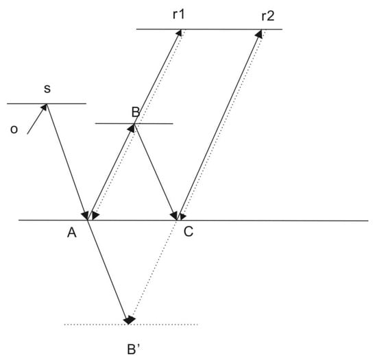
Figure 1.
The path of internal multiple and the generation of image artifacts. The nth-, (n + 1)th- and (n + 2)th-order internal multiples follow the path of o-s, s-A–B–r1, and B-C-r2. The nth-order internal multiple generates the (n + 1)th-order internal multiple, and the (n + 1)th-order internal multiple generates the (n + 2)th-order internal multiple. The dashed line r1-B-A and r2-C-B’ represents the path of backward-propagated wavefield of the (n + 1)th-order internal multiple and (n + 2)th-order internal multiple, respectively.
2.2. Internal Multiple Prediction Using High-Order Born Modeling
Here, the internal multiple prediction method we use is the high-order Born modeling method. This method obtains the predicted internal multiples in a forwarding process. The high-resolution velocity model and reflectivity model that are needed in the forwarding process can be provided and updated from LSRTM. This method provides separated forward-propagated internal multiples for LSRTM imaging.
In the theory of scattering series, we first get the wave equation of the actual velocity model and the reference velocity model:
where and is wavefield of the actual model and the reference model, and are the differential operators of the actual model and the reference model and satisfy:
The can be expressed as the wavefield of the reference reflectivity adding the scatter wavefield:
where is the scattering wavefield. Let the two equations of Equation (5) be subtracted, and let , where is the reflectivity model following, we can have:
Equation (8) describes how the scatter wavefield can be computed, However, We cannot get the value of in real cases, so we use as an approximate replacement of . We therefore have:
We use Equation (9) to compute . By continuously substituting into Equation (7) and substituting Equation (7) into Equation (8) to compute , we can get the internal multiple predicted by the high-order Born modeling method. The derivation is shown in Appendix A and the method is expressed as follows:
where is the scatter wavefield and can be written as the series , is the portion of that is ith order. The subscripts and represent the down- and upgoing components, and is the first-order internal multiple we need to calculate. is the zeroing matrix and is expressed as:
where is a threshold associated with . Therefore, we set:
where is the threshold parameter. Here we set the value of as 0.1.
2.3. LSRTM Image of Primary and Internal Multiples
LSRTM is also a method based on the Born modeling. Writing Equation (9) as the differential form, we have:
where is corresponding background wavefield, is the scatter wavefield.
The objective function of the LSRTM can be defined as:
where is the Born modeling operator defined in the equation (14) and is the recorded data.
Then we can get the gradient:
where is adjoint of , is the backward-propagated wavefield of the data residuals.
In this paper, the Laplacian filtering of the calculated gradient is needed to remove the low frequency components of the gradient. And the optimal method we choose is the limited-memory Broyden—Fletcher—Goldfarb—Shanno (l-BFGS) method [47].
According to Equation (4), we can obtain the correct image:
Due to the amplitude of higher-order internal multiple being low, we only consider the first-order internal multiple. Ignore higher order terms:
In order to meet the requirement of cross-correlation of corresponding-orders internal multiples in the image condition, we introduced the weighting matrix, and the objective function is changed to:
where represents the weighted matrix to select the primary and represents the weighted matrix to select the internal multiples. and is designed to separate the primary or multiple by given different weighting according to the observed data and the predicted internal multiple. Here, we set:
where and represent the value of and when the coordinate is , represents the normalized predicted internal multiples, represents the normalized observed data, and , is a threshold parameter.
Through introducing the weighting matrix, we can select the wave we need. The weighting matrix is set to a value of 1 at the position of the wave we need and a minimum value at the position of the wave we do not need. Where the value of is calculated as 1, the useful content is the primary and the internal multiples could be suppressed; where the value of is calculated as 1, the useful content are internal multiples and the primary could be suppressed. By building a division formula, we can set the values of and as we want.
Both LSRTM and the multiple prediction method are also based on the Born modeling theory, so they can use each other’s parameters. Thus, the calculation of the scatter wavefield requires LSRTM to provide an accurate reflectivity . However, There may be a difference in phase between actual reflectivity and the reflectivity provided by LSRTM. Thus, the internal multiples we compute may differ from the observed data in the phase and position. Using the computed weighting matrix to suppress them may not completely suppress the internal multiples. Thus, we use the Hilbert transforms in order to use the low frequency component of the predicted internal multiples and observed data to compute . The mismatch of the predicted internal multiples occurs mainly in the high frequency part, so introducing the Hilbert transform can reduce the influence of the mismatch. Then Equations (19) and (20) can be changed as:
Because the cross-correlation of the nth-order internal multiples in the forward- propagated wavefield and the backward-propagated wavefield of the nth-order internal multiples can create two correct images. Thus, the equation of the gradient should contain two terms related to the internal multiple.
According to the second part and third part of equation , , we can get the gradient:
where, is the upward of the primary and is the downward of the first-order internal multiple. To realize it, we have:
Thus, we can conduct the LSRTM process using the weighting matrix to realize the internal multiples, as Figure 2 shows.
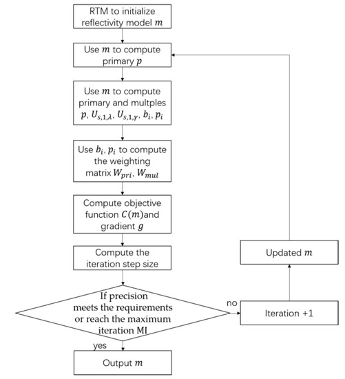
Figure 2.
Flow chart of the LSRTM image of primary and internal multiples.
3. Numerical Tests
In this section, we use the three-layer model and two-dimensional salt hill model to do the numerical test. And Table 1 shows our experiment and analysis.

Table 1.
The main content and conclusion of the numerical test.
3.1. Examples of Three-Layer Model
We used a three-layer model to test our method. Figure 3a illustrates the true velocity model. The model grid was 150 × 300 and the mesh spacing was 12.5 m. A total of 60 shots were evenly distributed on the surface, and the shot interval was 62.5 m. There were 300 receivers evenly distributed on the surface, and the receiver interval was 12.5 m. The source wavelet was selected as the Ricker wavelet with a peak frequency of 15 Hz. The time sample interval was 1 ms. Figure 3b illustrates the true reflectivity model, which can be a comparison of the LSRTM image.
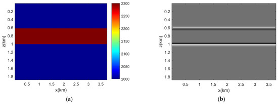
Figure 3.
(a) True velocity model. (b) True reflectivity model.
Here we choose the data of the 30th shot. The recorded data is shown in Figure 4a. Figure 4b shows the predicted internal multiples after five iterations. The predicted internal multiples are used for computing the weighting matrix to separate the primary and internal multiples in data residual. The data residual after five iterations is shown in Figure 4c. Figure 4d,e shows the primary and internal multiples of the data residual after using the weighting matrix, respectively. Due to the amplitude of the internal multiple being too small, the boundary reflection still exists in the shown data. The red arrows indicates the place of internal multiple. The internal multiple is about 1.5 s when the x-axis is 0 km. We can find the internal multiple in Figure 4a–c, e, which shows that it has been estimated and is separated from the data residual.
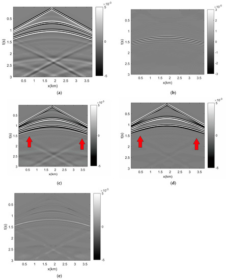
Figure 4.
(a) Recorded data. (b) Predicted internal multiples after five iterations. (c) The data residual after five iterations. (d) The primary of data residual after using the weighting matrix (e) The internal multiples of data residual after using the weighting matrix.
Figure 5 shows the images of the migration. As seen in Figure 5a, there are the artifacts in LSRTM image, and its depth is 1.4 km. These artifacts are suppressed in RWLSRTM image of the primary and RWLSRTM image of the primary and internal multiples, as shown in Figure 5b,c. Comparing Figure 5b,c, there are no other artifacts introduced. Figure 5d,e is the comparison of the 150th trace and its extract of the depth of 1.25 km and 1.875 km. We can see the artifacts at a depth of about 1.4 km only exist in the LSRTM and is eliminated when the internal multiple is separated.
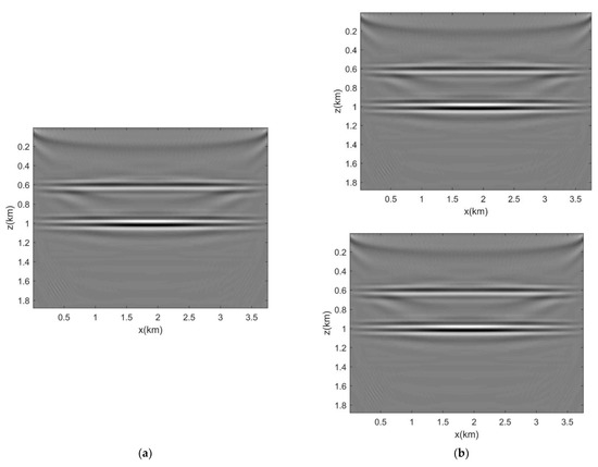
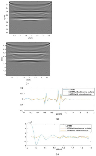
Figure 5.
(a) LSRTM image. (b) RWLSRTM image of the primary. (c) RWLSRTM image of the primary and internal multiples. (d) the comparison of 150th trace (e) the comparison of 150th trace deeper than 1.25 km.
3.2. Examples of Two-Dimensional Salt Hill Model
The two-dimensional Salt Hill model was used in the numeric test in this paper, and the true velocity model and reflectivity model is shown in Figure 6. The model grid was 150 × 644 and the mesh spacing was 12.5 m. A total of 70 shots and 645 receivers were evenly distributed on the surface. The shot interval was 112.5 m and the receiver interval was 12.5 m. The source wavelet was selected as the Ricker wavelet with a peak frequency of 15 Hz.
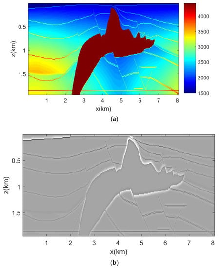
Figure 6.
(a) True velocity model. (b) True reflectivity model.
Figure 6a is the velocity model and Figure 6b is the reflectivity model, which can be a comparison of the LSRTM image. Figure 7a shows the recorded data. Figure 7b shows the predicted internal multiples after five iterations. Figure 7c shows the primary of the data residual after using the weighting matrix. Figure 7d shows the internal multiples of data residual after using the weighting matrix. We can find the internal multiple in Figure 4a,b,d, that shows that it has been estimated, and is separated from the data residual. Figure 4e is the waveform comparison of the data residual and the data residual of the primary and internal multiple. Through comparison, we can find the multiple existing mainly in about 0.8 s, the energy of the multiple is low when the energy of the primary is strong, and the energy of the multiple is strong when the energy of the primary is weak. Therefore, we can say that the primary and multiple are separated in the data residual.
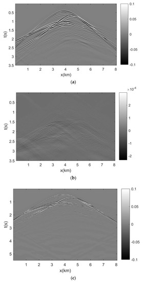
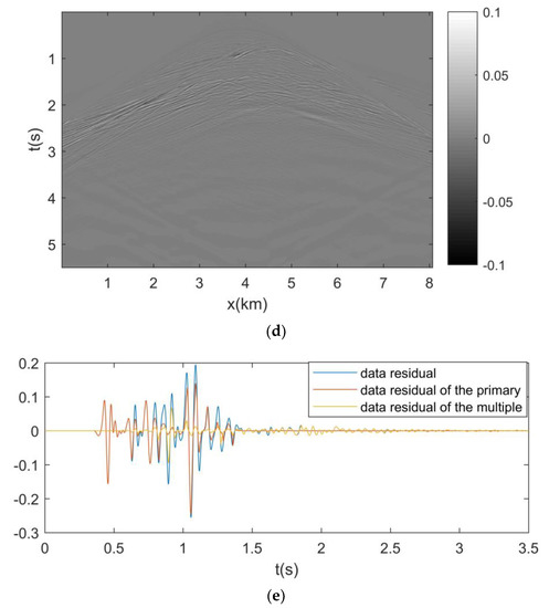
Figure 7.
(a) Recorded data. (b) Predicted internal multiples after five iterations. (c) The primary of data residual after using the weighting matrix. (d) The internal multiple of data residual after using the weighting matrix. (e) Waveform comparison of data residual and data residual of primary and internal multiple.
Figure 8a,c,e show the LSRTM image, the RWLSRTM image of the primary, and the RWLSRTM image of the primary and internal multiples. Figure 8b,d,f shows their close-up section. The red arrows of letter A and B indicate artifacts caused by the internal multiples in Figure 8a, and they are suppressed in Figure 8b,c. The artifacts caused by the internal multiples in the image by the primary were depressed. Without the interference of artifacts, the actual structure has better convergence and looks clearer, as the place that the letter C points out in Figure 8. However, the actual structure in the image by the primary was also depressed, as indicated below letter B. In the image by the primary and internal multiples, the actual structure was compensated. Because the artifacts were suppressed, the overlap between the actual structure and the artifact was also suppressed, which made the actual structure discontinuous. In addition, it did not introduce the artifacts in the image when the primary and the internal multiple were separated in the image, as indicated by the letter B.
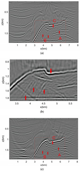
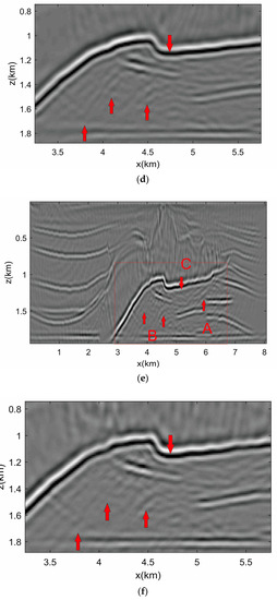
Figure 8.
(a) LSRTM image. (b) Close-up section of LSRTM image. (c) RWLSRTM image of the primary. (d) Close-up section of RWLSRTM image of the primary. (e) RWLSRTM image of the primary and internal multiples. (f) Close-up section of RWLSRTM image of the primary and internal multiples.
We chose the 290th trace and the 320th trace to compare their image, as Figure 9a,b show. The 290th trace is indicated by the far left arrow in Figure 8f. In Figure 9a, the useful structure is at about 1.6 km. Only the LSRTM without the internal multiple did not image here, and this shows that the internal multiples contain some information of useful structure and can be a good complement in image. The 320th trace is about the second arrow in the left in Figure 8f. In Figure 9b, the artifact is about in 1.4 km. Only the LSRTM contains the artifacts, and shows that it is effective in reducing the artifacts when separating the internal multiples.
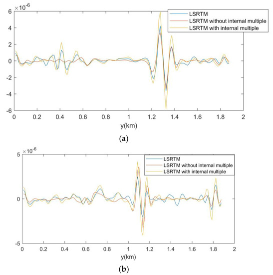
Figure 9.
(a) the comparison of the 290th trace. (b) the comparison of the 320th trace.
4. Conclusions
We realized the image by the primary and internal multiples based on internal multiple prediction using high-order Born modeling in the LSRTM. The internal multiple prediction using high-order Born modeling predicted the internal multiples in the forwarding process in the time domain. We established the objective function according to the RWLSRTM. By introducing the weighted matrix, we separated the primary and internal multiples and imaged them. Through the numerical test, we found the artifacts caused by the internal multiples that could be suppressed, and the actual structure was compensated. This made the actual structure more obvious, and the artifacts interference could be suppressed.
The method still has disadvantages. The overlap of the artifacts and the actual structure was also suppressed. This caused the actual structure to have some discontinuity points. Second, because of the property of the zeroing matrix we used in high-order Born modeling, the internal multiples of two close reflective layers may not be predicted well. Perhaps we can find a better way to realize the high-order Born modeling in the time domain and get a more precise result.
Author Contributions
Conceptualization, R.C., L.H. and P.Z.; methodology, R.C.; formal analysis, R.C. and P.Z.; writing—original draft preparation, R.C.; writing—review and editing, L.H. and P.Z. All authors have read and agreed to the published version of the manuscript.
Funding
This research was funded by the National Natural Science Foundation of China (No. 42130805, No. 42074154, No. 42004106, ), the Lift Project for Young Science and Technology Talents of Jilin Province (No. QT202116).
Institutional Review Board Statement
Not applicable.
Informed Consent Statement
Not applicable.
Data Availability Statement
Not applicable.
Conflicts of Interest
The authors declare that they have no conflict of interest.
Appendix A
The scattering wavefield can be written as the series:
is the portion of that is ith order. And we can write Equation (9) as:
Use as an approximate replacement of . Substitute into Equation (7) and substitute Equation (7) into Equation (8), and we can have:
So we can get:
Use and approximate replacement of . Substitute into Equation (7) and substitute Equation (7) into Equation (8) again, we can have:
The represents the wavefield experiencing scattering for three times. The first-order internal multiple is also the wavefield that experienced scattering for three times and contained in the . The propagation of the first-order internal multiple is down-up-down, so we can get the first order internal multiple when meets the depth condition of , where , , is the depth of the first, second, and third scatter point. Here we do wavefield decomposition to meet the depth condition. Then we can get:
The subscripts and indicate that the propagation of the wavefield is down and up. Subscripts 1 and 2 indicate that the scatter wavefields is first and second order.
In Figure A1 is the wavefield, and the subscripts indicate that the propagation of the wavefield is rightward, and is generated by according to Equation (A.6). Through Figure 2 we see that makes the virtual source of still exist in . In other words, there is overlap of and . In this case, the depth condition can only reach . To solve this problem, we need not only to split the up- and downgoing wavefields but also to introduce the zeroing matrix to remove the overlap of and . Then we can get:

Figure A1.
Wave field after wave decomposition.
Figure A1.
Wave field after wave decomposition.

The zeroing matrix is expressed as:
where is a threshold parameter. The setting of the threshold should separate the wavefield with the stronger energy and the others, while , which we need, cannot be removed. In the overlap of and , the i-th order scatter wavefield has far more energy than the lower order scatter wavefield. Thus, we can let the associate with the maximum value of the virtual source of , then we can get:
where is the threshold parameter. If the value of is set too high, the overlap may not be removed clearly; if the value of is set too low, the wavefield we need maybe removed. Thus, we need to set a suitable value. Here we can set a relatively higher value, and about one-quarter to half a cycle before and after the wavefield part that meets the threshold is reset to zero. Thus, we get:
This can separate the overlap better. However, the internal multiple couldn’t be predicted if the reflection interface is too close.
References
- Hampson, D. Inverse Velocity Stacking for Multiple Elimination. In Proceedings of the 56th Annual International Meeting, SEG Expanded Abstracts, Houston, TX, USA, 2–6 November 1986; pp. 422–424. [Google Scholar]
- Schneider, W.A.; Backus, M.M. Dynamic correlation analysis. Geophysics 1968, 33, 105–126. [Google Scholar] [CrossRef]
- Taner, M.T.; Koehler, F. Velocity spectra-digital computer derivation and applications of velocity functions. Geophysics 1969, 34, 859–881. [Google Scholar] [CrossRef]
- Robinson, E.A. Predictive decomposition of seismic trace. Geophysics 1957, 22, 767–778. [Google Scholar] [CrossRef]
- Backus, M.M. Water reverberation: Their nature and elimination. Geophysics 1959, 24, 233–261. [Google Scholar] [CrossRef]
- Ryu, J.V. Decomposition (DECOM) approach applied to wave field analysis with seismic reflection records. Geophysics 1982, 47, 869–883. [Google Scholar] [CrossRef]
- Yilmaz, O. Seismic Data Processing; Electronic Edition; Society of Exploration Geophysicists: Tulsa, OK, USA, 1987. [Google Scholar]
- Foster, D.J.; Mosher, C.C. Suppression of multiple reflections using the Radon transform. Geophysics 1992, 57, 386–395. [Google Scholar] [CrossRef]
- Jakubowicz, H. Wave equation prediction and removal of interbed multiples. In Proceedings of the 68th Annual International Meeting, SEG Expanded Abstracts, New Orleans, LA, USA, 13–18 September 1998; pp. 1527–1530. [Google Scholar]
- Verschuur, D.J.; Berkhout, A.J. Removal of internal multiples with the common- focus-point (CFP) approach: Part 2—Application strategies and data examples. Geophysics 2005, 70, V61–V72. [Google Scholar] [CrossRef]
- Ikelle, L.T. A construct of internal multiples form surface data only: The concept of virtual seismic events. Geophysics 2006, 164, 383–393. [Google Scholar]
- Ikelle, L.T. Scattering diagrams in seismic imaging: More insights into the construction of virtual events and internal multiples. J. Appl. Geophys. 2009, 67, 150–170. [Google Scholar] [CrossRef]
- Yuan, S.; Wang, S.; Yuan, F.; Liu, Y. The influence of errors in the source wavelet on inversion-based surface-related multiple attenuation. Geophys. Prospect. 2018, 66, 55–73. [Google Scholar] [CrossRef]
- Carvalho, F.M.; Weglein, A.B.; Stolt, R.H. Examples of a non-linear inversion method based on the T matrix of scattering theory: Application to multiple suppression. In Proceedings of the 61st Annual International Meeting, SEG Expanded Abstracts, Houston, CA, USA, 10–14 November 1991; pp. 1319–1322. [Google Scholar]
- Carvalho, F.M.; Weglein, A.B.; Stolt, R.H. Non-linear inverse scattering for multiple suppression: Application to real data, Part I. In Proceedings of the 62nd Annual International Meeting, SEG Expanded Abstracts, New Orleans, LA, USA, 25–29 October 1992; pp. 1093–1095. [Google Scholar]
- Carvalho, F.M. Free-Surface Multiple Reflection Elimination Method Based on Non-Linear Inversion of Seismic Data. Ph.D. Dissertation, Universidade Federal da Bahia, Salvador, Brazil, 1992. (In Portuguese). [Google Scholar]
- Weglein, A.B.; Gasparotto, E.A.; Carvalho, P.M.; Stolt, R.H. An inverse-scattering series method for attenuating multiples in seismic reflection data. Geophysics 1997, 62, 1975–1989. [Google Scholar] [CrossRef]
- Weglein, A.B. Multiple attenuation: An overview of recent advances and the road ahead. Lead. Edge 1999, 18, 40–44. [Google Scholar] [CrossRef]
- Matson, K.H. The relationship between seattering theory and the Primaries and multiples of refiection seismic data. J. Seism. Explor. 1996, 5, 63–78. [Google Scholar]
- Matson, K.H. An inverses scattering series method for attenuating elastic multiples from multicomponent land ocean bottom seismic data. Ph.D. Dissertation, Dept. EOAS., British Columbia Univ. B.C., Vancouver, BC, Canada, 1997. [Google Scholar]
- Ikelle, L.T. Using even terms of the scattering series for deghosting and multiple attenuation of ocean-bottom cable data. Geophysics 1999, 64, 579–592. [Google Scholar] [CrossRef]
- Ramírez, A.C.; Weglein, A.B. An inverse scattering internal multiple elimination method: Beyond attenuation, a new algorithm, and initial tests. In Proceedings of the 75th Annual International Meeting, SEG Expanded Abstracts, Houston, TX, USA, 6–11 November 2005; pp. 2115–2118. [Google Scholar]
- Pica, A.; Laurie, D. Wave equation based internal multiple modeling in 3D. In Proceedings of the 78th Annual International Meeting, SEG Expanded Abstracts, Las Vegas, NV, USA, 9–14 November 2008; pp. 2476–2480. [Google Scholar]
- van der Neut, J.; Wapenaar, K. Adaptive overburden elimination with the multidimensional Marchenko equation. Geophysics 2016, 81, T265–T284. [Google Scholar] [CrossRef]
- Berkhout, A.J. Combining full wavefield migration and full waveform inversion. In Proceedings of the 81st Annual International Meeting, SEG Expanded Abstracts, San Antonio, TX, USA, 18–23 September 2011; pp. 3321–3325. [Google Scholar]
- Berkhout, A.J. Combining full wavefield migration and full waveform inversion, a glance into the future of seismic imaging. Geophysics 2012, 77, S43–S50. [Google Scholar] [CrossRef]
- Berkhout, A.J. Review Paper: An outlook on the future of seismic imaging, Part II: Full-Wavefield Migration. Geophys. Prospect. 2014, 62, 931–949. [Google Scholar] [CrossRef]
- Whitmore, N.D. Iterative depth migration by backward time propagation. In Proceedings of the 53rd Annual International Meeting, SEG Expanded Abstracts, Las Vegas, NV, USA, 11–15 September 1983; pp. 382–385. [Google Scholar]
- Moradpouri, F.; Moradzadeh, A.; Pestana, R.C. Seismic reverse time migration using a new wave-field extrapolator and a new imaging condition. Acta Geophys. 2016, 64, 1673–1690. [Google Scholar] [CrossRef]
- Moradpouri, F.; Moradzadeh, A.; Pestana, R.N.C.; Ghaedrahmati, R.; Soleimani, M. An improvement in wave-field extrapolation and imaging condition to suppress RTM artifacts. Geophysics 2017, 82, S403–S409. [Google Scholar] [CrossRef]
- Soleimani, M. Challenges of seismic imaging in complex media around Iran, from Zagros overthrust in the southwest to Gorgan Plain in the northeast. Lead. Edge 2017, 36, 499–506. [Google Scholar] [CrossRef]
- Moradpouri, F. A new approach in reverse time migration for properly imaging complex geological media. Acta Geophys. 2021, 69, 529–538. [Google Scholar] [CrossRef]
- Tarantola, A. Linearized Inversion of Seismic Reflection Data. Geophys. Prospect. 1984, 32, 998–1015. [Google Scholar] [CrossRef]
- Dai, W.; Wang, X.; Schuster, G.T. Least-squares migration of multisource data with a deblurring filter. Geophysics 2011, 76, R135–R146. [Google Scholar] [CrossRef]
- He, R.; Schuster, G. Least-squares migration of both primaries and multiples. In Proceedings of the 73rd Annual International Meeting, SEG Expanded Abstracts, Dallas, TX, USA, 26–31 October 2003; pp. 1035–1038. [Google Scholar]
- Liu, Y.; Xu, C.; Jin, D.; He, R.; Sun, H.; Zheng, R. Reverse time migration of multiples. In Proceedings of the 81st Annual International Meeting, SEG Expanded Abstracts, San Antonio, TX, USA, 18–23 September 2011; pp. 3326–3331. [Google Scholar]
- Liu, Y.; Xu, C.; Jin, D.; He, R.; Sun, H.; Zheng, R. Reverse time migration of multiples for subsalt imaging. Geophysics 2011, 76, WB209–WB216. [Google Scholar] [CrossRef]
- Zhang, D.; Schuster, G.T. Least-squares reverse time migration of multiples. Geophysics 2014, 79, S11–S21. [Google Scholar] [CrossRef]
- Liu, X.; Liu, Y.; Khan, M. Fast least-squares reverse time migration of VSP free-surface multiples with dynamic phase-encoding schemes. Geophysics 2018, 83, S321–S332. [Google Scholar] [CrossRef]
- Li, Z.; Li, Z.; Li, Q.; Li, Q.; Sun, M.; Hu, P.; Li, L. Least-squares reverse time migration of multiples in visco-acoustic media. Geophysics 2020, 85, S285–S297. [Google Scholar] [CrossRef]
- Wong, M.; Biondi, B.; Ronen, S. Imaging with primaries and free-surface multiples by joint least-squares reverse time migration. Geophysics 2015, 80, S223–S235. [Google Scholar] [CrossRef]
- Liu, X.; Liu, Y. Plane-wave domain least-squares reverse time migration with free-surface multiples. Geophysics 2018, 83, S477–S487. [Google Scholar] [CrossRef]
- Qu, Y.; Huang, C.; Liu, C.; Li, Z. Full-Path Compensated Least-Squares Reverse Time Migration of Joint Primaries and Different-Order Multiples for Deep-Marine Environment. IEEE Trans. Geosci. Remote Sens. 2021, 59, 7109–7121. [Google Scholar] [CrossRef]
- Liu, Y.; Liu, X.; Osen, A.; Shao, Y.; Hu, H.; Zheng, Y. Least-squares reverse time migration using controlled-order multiple reflections. Geophysics 2016, 81, S347–S357. [Google Scholar] [CrossRef]
- Li, C.; Huang, J.; Li, Z.; Yu, H.; Wang, R. Least-squares migration with primary- and multiple-guided weighting matrices. Geophysics 2019, 84, S171–S185. [Google Scholar] [CrossRef]
- Chen, R.; Han, L.; Zhang, P.; Dong, S.; Yin, Y. Internal multiple prediction using high-order born modeling for LSRTM. Acta Geophys. 2022, 70, 1491–1505. [Google Scholar] [CrossRef]
- Nocedal, J. Updating quasi-Newton matrices with limited storage. Math. Comput. 1980, 35, 773–782. [Google Scholar] [CrossRef]


Publisher’s Note: MDPI stays neutral with regard to jurisdictional claims in published maps and institutional affiliations. |
© 2022 by the authors. Licensee MDPI, Basel, Switzerland. This article is an open access article distributed under the terms and conditions of the Creative Commons Attribution (CC BY) license (https://creativecommons.org/licenses/by/4.0/).