Abstract
In aquaculture, new production technologies are under development and testing. One promising type of technology is the closed floating cage. Egget® is one of these newly developed technologies, which is egg-shaped and vertically floating. One of the challenges is to determine hydrodynamic loads. Therefore, this study focuses on estimating the resistance and the resistance coefficient for steady flow with various velocities and Reynolds numbers on a scaled model. It includes simulations using Computational Fluid Dynamics (CFD) for two depths and experiments in the MarinLab at Western Norway University of Applied Sciences (HVL). As the cage is partially submerged, the simulations are performed using the Volume of Fluid (VOF) technique for modeling free surface flow. The comparison of experimental and simulation results show good agreement.
1. Introduction
Aquaculture is growing and new production technologies are under development and testing. While open net pens are the standard equipment, one opportunity for controlling the environment and reduce the risk of fish escape is to close the fish farm unit from the surroundings using firm walls. Egget® is an example of this, which utilizes a fiber composite structure. Cylindrical closed fish farms have lately received much focus, for example, in [1,2], where the researchers have carried out experiments and numerical analysis with a particular emphasis on the sloshing behavior. While Egget® has certain similarities to the structure studied, it has the shape of an Egg with a cylindrical buoyancy collar attached to it. To establish the hydrodynamic response and loads, precise estimates of the hydrodynamic properties are crucial. The total resistance includes all contributions, including wave making resistance. The resistance coefficient is used to estimate force from wind and current or, together with the inertia coefficient, to calculate wave loads, for example, by applying the well known Morison equation [3] for estimates of wave forces on slender structures. Achenbach [4] studied the pressures and skin friction on the surface of cylinders with different surface roughness exposed to a constant flow in an air duct. He published data for skin friction, drag coefficients and separation points for a range of Reynolds numbers between and . The study showed that the Reynolds number at which the critical flow sets in, as well as the level of drag in a certain flow regime, is impacted by the surface roughness. Achenbach further published a study for smooth spheres, where drag coefficients are documented for the Reynolds numbers between and [5]. Sarpkaya [6] published results from experiments in an u-shaped tube filled with water and different cylinders mounted on force measurement devices in the middle section. By oscillating the water and measuring the force, the drag and inertia coefficients for different cylinders was established for Reynolds numbers up to . His results demonstrated that the drag and inertia coefficients depend on velocity and wave period as well as viscosity and diameter. James et al. provided experimental results for the flow around a sphere towed at the water surface in a conference paper [7] at Reynolds numbers between and , where drag coefficients are reported. Chaplin and Teigen [8] reported on experiments on a standing tube instrumented with pressure transducers and towed through a basin. The results demonstrated that the resistance coefficient depends on the proximity to the waterline as a function of the Froude number. They provide resistance coefficients for a vertical tube extending 2 diameters into the water volume. Ren et al. [9] focused on hydrodynamic forces on partially submerged horizontal cylinders with Reynolds numbers ranging from to . Their experimental results showed that when the cylinder protrudes the surface, the drag crisis did not occur as for completely submerged cylinders. They observed a reduction in drag coefficient as the depth decreased, which is not linear to the change in cross section area. This is indicative of a surface effect on the force measurement. Further they observed a dependence of the Froude number on the drag force. Although it is common to study flow problems based on similarity in Reynolds number, resistance tests for ships are usually carried out by Froude scaling, since this enables calculation of the wave making resistance [10]. To validate the experimental results and for analysis of similar and complex shapes, proper numerical models are important. Liang et al. applied the finite difference method to estimate the drag force and drag coefficient [11]. In other attempts, [12,13] performed a CFD analysis and got a good agreement between numerical and experimental results. In a similar case to this study topic, Cheng et al. in [14] showed that the drag coefficient of an elliptical section is 51.3% smaller than for a circular section using the finite volume method. CFD simulations for partially submerged objects are often carried out for a transient state using the subgrid-scale model (SGS) and Large Eddy Simulation (LES) [15] with the free surface approach. However, for special cases where the Froude number is small, the free surface may be replaced by a surface with zero shear stress [8].
This study aims to develop a CFD numerical model to estimate the resistance and coefficients on an egg-shaped dome (tank). The tank is a combination of cylindrical and ellipsoidal shapes, which makes it difficult to compare the hydrodynamic loads with available research. The developed CFD model utilizes the Volume of Fluid (VOF) technique and Reynolds averaged equations, which allows for the simulation of free surface flow over a partially submerged dome. The developed model may be an alternative to the large computational effort transient SGS model. The numerical results are validated with experimental data. A reliable numerical model can be utilized for full-scale cases with any changes in the geometry and environmental conditions.
2. Materials and Methods
2.1. CFD Method
The equations that describe the motion of fluid are called the Navier–Stokes equations and consist of two equations, the mass conservation equation [16]:
and the momentum conservation equation
where is fluid density, p is pressure, u is fluid velocity, is a stress tensor, is fluid viscosity, I is unit tensor, is gravity, is external force, Q is the fluid source, and is the external momentum source.
The solution of the N-S equations in general form, even numerically, would be computationally expensive for turbulent flows, which by definition is random by nature. Therefore, one of the widely used approaches in Computational Fluid Dynamics is to replace instantaneous variables with time-averaged (mean) values and their fluctuations. Any scalar quantities can be presented by
where is a mean (time-averaged) value and is the fluctuation over the mean value. This leads to the Reynolds Averaged N-S (RANS) equations in the form presented in the following. Assuming no mass transfer between fluid phases and no external forces act on the fluid, the source term in Equation (1) and the force in Equation (2) equals zero.The time averaged continuity equation in Cartesian coordinates is given by
and the time averaged momentum conservation equation is
The RANS equations remain open and the term , which is called Reynolds stress, must be modelled to close them. The most common approach is the Boussinesq approach, which defines the Reynolds stress to the gradient of mean fluid velocity gradient
where is the Kronecker delta:
The turbulence models use the Boussinesq approach, among which the most commonly used is k – , which, however, has weaknesses in modeling separating and swirling flow and is dedicated mainly to high-Reynolds number flows. Another turbulent model that eliminates mentioned drawbacks is a two-equation turbulence model, the k – . It also has a few modifications, among which the Shear Stress Transport () showed good agreement with flow over a cylinder, as it was proved in work [17]. This study uses the model to simulate flow over the egg-shaped tank.
The turbulence kinetic energy, k, in the model is expressed as
The specific dissipation rate is
where the effective diffusivities for k and are as follows
Here, and are the Prandtl numbers for k and , respectively, which are
and
The turbulent viscosity is given by
where S is the strain rate magnitude, and the low number correction coefficient is
where
where . For a high Reynolds number, . The blending functions and are defined as
and
where y is the distance to the next surface and is expressed as
The production of in Equation (11) is given by
and the dissipation of k and in Equations (9) and (11) is
and
The way how the flow is described near walls is included in wall functions. The standard wall function defines the mean velocity near the walls as:
where is a dimensionless velocity
and is a dimensionless distance from the wall
The simulation of free surface flow employs a technique of tracking the interface of two or more fluids known as a Volume of Fluid (VOF). This interface is predicted in an Eulerian grid for immiscible fluids by evaluation of the volume fraction of each phase inside the computational domain. The mass continuity Equation (1) for two phase flow without additional source flow and mass transfer between fluids will have the following form:
where is a volume fraction of the first fluid and the index denotes the number of fluids. The volume fraction is:
- 1, if a cell is fully occupied by fluid;
- 0, if a cell is not occupied by fluid;
- 0 < < 1 if there exists an interface between fluid 1 and 2.
The total forces calculated during fluid flow on a wall are calculated by
where k are cell surfaces belonging to the considered wall, and n is a normal vector to the cell surface. To be able to compare to other tests and similar objects, it is convenient to compute a total resistance coefficient, which is defined by
Here, A is chosen to be the front projected area in this study, since referred articles have used the same. For resistance testing it is also common to use the wetted surface area as described in [10]. For kinematic flow similarity below the water level, the Reynolds number, , should be equal for the experimental and numerical analysis. The Reynolds number is defined as
where is the dynamic viscosity and L is the diameter of the egg at the waterline. In addition, to achieve geometric and dynamic similarity, Froude scaling should be used. The Froude number, , depends on the gravitational acceleration, g, and is given by
For large full scale objects, it is impossible to both fulfill kinematic and dynamic similarity when scaling to a model test. Then, Froude scaling is more convenient, and trip tape is used at model scale to obtain flow similarity. For this study the CFD analysis is performed at model scale so that both and are kept equal to the experiment.
2.2. Experimental Setup
The experiments are carried out in the MarinLab at the Western Norway University of Applied Sciences. The lab consists of a tank of 50 × 3 × 2.2 m in length, width, and depth, respectively. An Edinburgh Designs wavemaker with six flaps and force feedback loop for noise reduction is installed on one end and a passive wave absorber on the other. Additionally, there is a carriage that is used to tow objects through the tank with various speed. The experimental setup can be seen in Figure 1, which is bears similarity to other studies on hydrodynamic loads on partially submerged objects [8,9].
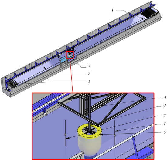
Figure 1.
The experimental setup: 1—wave absorber, 2—tested model on carriage, 3—wave generator, 4—towing carriage, 5—measurement beam, 6—tested model, 7—wave gauges.
The tested model is fixed at a stainless square section hollow profile with section length of 50 mm and thickness of 4 mm. It is instrumented with eight strain-gauges, in pairs of two in each direction and at two different levels, as illustrated in Figure 2. The strain gauges are connected in pairs to the measuring beam. Each pair is connected in a Wheatstone half-bridge to one of four input channels on a QuantumX MX440B data acquisition system, which is connected to the Catman Easy software. The data acquisition system records the signals at a rate of 150 Hz and stores results in ASCII text format. Before the experimental test, the measurement system is calibrated by applying predefined loads.
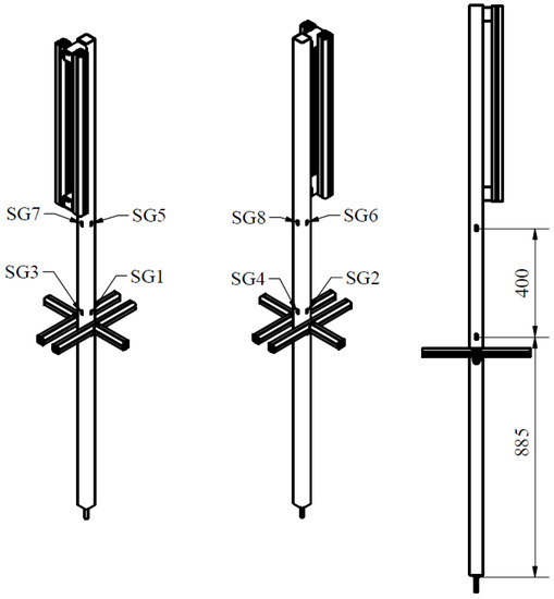
Figure 2.
Location of strain gauges SG1…SG8 on the measurement beam (item 5 in Figure 1, dimensions in [mm]).
2.3. Case Study
The subject of study is a concept demonstrator of the fish farm egg of approximately 2000 m volume, illustrated in Figure 3.
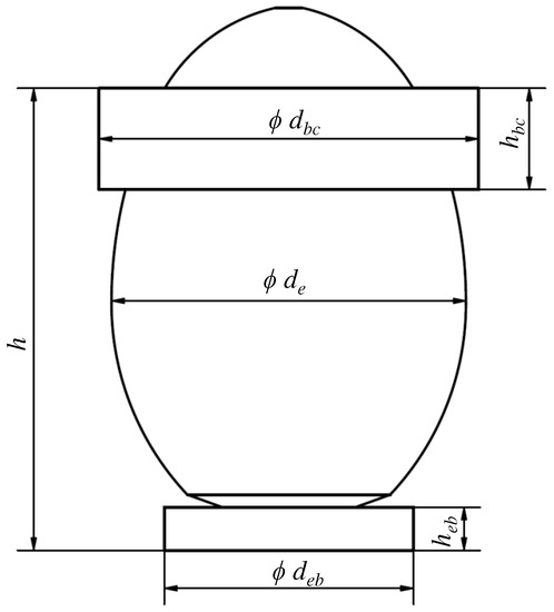
Figure 3.
The demonstrator of the fish farm egg.
The dimensions and other features of the egg demonstrator are presented in Table 1. It is worth noting that experiments are performed at water temperature 15 C and draught , while as CFD calculations are performed at water temperature 20 C and .

Table 1.
The egg demonstrator dimensions.
2.4. Experimental Procedure
For each experiment, the carriage velocity is manually set, and the experiment is repeated three times with approximately 20 min of waiting time between each test to ensure the water is sufficiently calm before starting the test. Two stationary segments of measurements are extracted from each experiment for analysis—one before the motion commenced and one from a stationary segment after the pre-determined velocity is reached. For each of these, the signals are filtered through a Butterworth low-pass filter of order 10 with a cut-off frequency of 2.5 Hz. The total resistance is calculated based on recorded strain gauges located on the measuring beam. The experimental tests are conducted in the way that the carriage is accelerated to the required speed, and then the speed is maintained for a specific period until the end of the tank could affect the flow. The entire procedure, i.e., acceleration, constant speed and deceleration is recorded; however, only the mean total resistance for the period with constant speed is evaluated. This can be seen as phase III in the example shown in Figure 4.
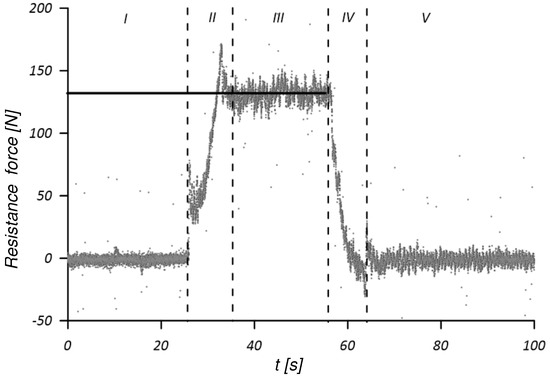
Figure 4.
An example of measurement, I, V—idle phases, II—acceleration to required speed, III—constant speed, IV—deceleration.
A 95% confidence interval is established [18], from the three repetitions of each experiment by assuming a student’s t-distribution. The mathematical formulation is given by
where and denotes the experimental value and its mean, is its standard deviation, is a measure for the number of standard deviations to add or subtract. With three repetitions, and C = 95%, . The resulting confidence intervals are shown in the Results section together with the mean resistance values.
2.5. CFD Model
The CFD simulation is conducted in Ansys Fluent CFD package with the use of VOF (Volume of Fluid) technique. Despite the fact that the VOF method is generally dedicated to time-dependent analysis, the steady state condition simulation is implemented. The initial interface between both phases (air and water) is known, and both fluids do not interpenetrate each other in a substantial matter. The fluid properties are given in Table 2 and the following assumptions are taken during the simulations:
Table 2.
Fluid properties.
- both fluids are incompressible and homogeneous;
- both fluids have constant properties;
- there is no mass transfer between both fluids;
- model is in thermal equilibrium;
- phase changes in both fluids are neglected;
- the pressure-based solver is used;
- for the pressure-velocity the coupled scheme linked to the volume fraction is used;
- the implicit scheme is used with a standard finite difference discretization scheme: QUICK and Modified HIRC for volume fraction;
- the shear stress transport (SST) model is used;
- the roughness of model wall is neglected.
The CFD model, shown in Figure 5, is prepared for steady-state conditions with a fixed position of the egg model and forced fluid flow. In contrast, experimental tests are conducted for the moving model. Therefore, the CFD model’s boundary conditions are specified to reflect experimental test conditions. The tank side walls are considered frictionless, i.e., the shear stresses are set to 0. The size of the fluid domain is chosen so that the flow field is not affected by boundary conditions. The domain is equivalent to the tank cross section dimensions of the MarinLab and the domain length from the inlet to the dome wall is four times larger than the dome diameter, while to the outlet it is approximately ten times the dome diameter. Additionally, half of the model is used. The simulations aimed to calculate the total resistance force and total resistance coefficient for different velocities and draught.
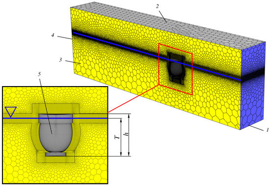
Figure 5.
CFD model: 1—pressure inlet (open channel), 2—pressure outlet, 3—symmetry, 4—pressure outlet (open channel), 5—wall, T—draught.
The computational model is prepared with mixed cell types: polyhedral and hexahedral. The predicted interface between water and fluid is refined, as well as a region near the egg walls. The grid is locally refined to capture flow induced on the egg wall during fluid flow. The total number of cells is approximately 1.5 × 10. Figure 6 shows a grid sensitivity study.
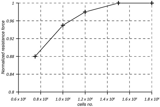
Figure 6.
Grid sensitivity.
The refined grid on a dome achieving values below 200 is shown in Figure 7.
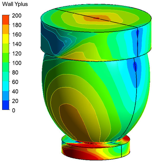
Figure 7.
The value.
3. Results
The mean value and resulting confidence interval of the measured resistance, along with the CFD simulation results, are presented in Figure 8. CFD simulations are also conducted for two different draughts: and .
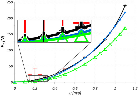
Figure 8.
Total resistance : Experiments (+), CFD (•), CFD (Δ), the red bar is the uncertainty.
The obtained forces are next used to evaluate the total resistance coefficient vs. Reynolds number using Equations (31) and (32). The Figure 9 below shows the total resistance coefficient () as a function of the Reynolds number ().
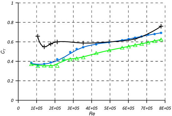
Figure 9.
Total resistance coeff. : Experiments (+), CFD (•), CFD (Δ).
The experimental test is also recorded, allowing for comparison of the water free surface with the CFD simulations. Figure 10 shows the free surface comparison between experimental tests and the one obtained in CFD simulations for the carriage velocity of 1.1 m/s, corresponding to . The white region shows the front wave induced by the model, while the red area shows high vorticity.
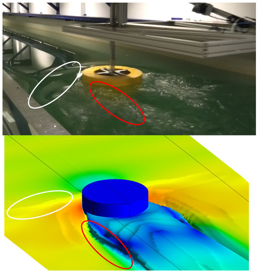
Figure 10.
Water free surface; top—experiments, bottom—CFD.
Figure 11 and Figure 12 show water velocity and vorticity on a symmetry plane, respectively. Figure 13 shows water fraction at the symmetry plane while Figure 14 shows 3D streamlines colored by water velocity.
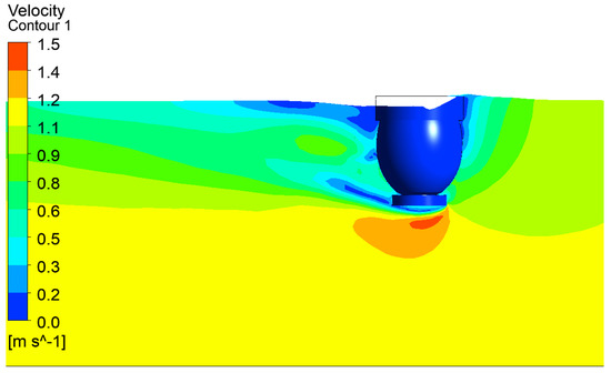
Figure 11.
CFD results on the symmetry plane for : water velocity.
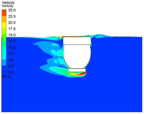
Figure 12.
CFD results on the symmetry plane for : water vorticity.
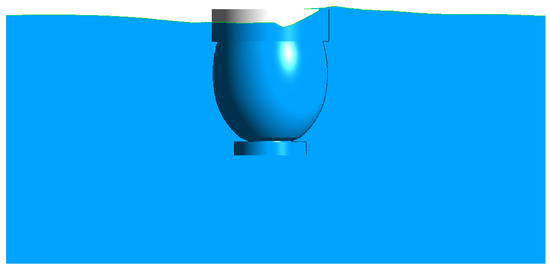
Figure 13.
CFD results on the symmetry plane for : water fraction.
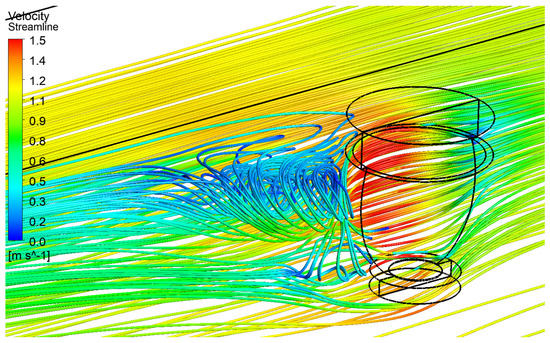
Figure 14.
CFD results : 3D streamlines for water fraction.
4. Discussion
The comparison of CFD results and experimental tests in terms of total resistance value (Figure 8), total resistance coefficient (Figure 9), and shape of water free surface (Figure 10) show good agreement for . It is achieved despite the simulations conducted for steady state conditions and using the Reynolds averaging approach. It should be underlined that a good agreement between simulations and experimental tests is obtained for the water free surface for . In the marked regions in Figure 10, nearly identical shapes of induced front wave can be observed (region marked white). The high wake region can also be observed in the same location in the CFD model and experimental tests (region marked red). More differences appear with smaller numbers, i.e., between and , possibly due to the Reynolds averaging approach and steady-state simulation. The values for were not compared due to the uncertainty level for experimental tests.
It can be observed that the total resistance coefficient depends on the draught value. It is consistent with other studies; although a majority of them relate to the high ratio T/D (draught to cylinder diameter) of vertical cylinders, similar trends can be observed [15,19]. One of the few studies on similar cases (low aspect ratio) [20] also show that the total resistance coefficient is directly dependent on the draught. Figure 3 in [20] indicates that the total resistance coefficient varies depending on the cylinder diameter (tests were conducted for the constant draught), i.e., depending on the T/D ratio. It is also confirmed for the test at cylinders with a low aspect ratio, as presented in Figure 6 in study [15]. The work [21] presents the results of drag coefficient research for a fully immersed cylinder. However, it can be seen that the drag coefficient is almost constant to some range of . This graph cannot be used as a reference to the presented case study, but in principle, a similar trend should be expected for the investigated egg-shaped dome. The total resistance coefficient value of the egg-shaped dome is expected to be smaller than those presented in Figure 15.
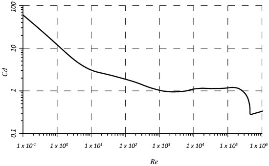
Figure 15.
Drag coefficient for fully immersed cylinder. The figure is prepared based on [21].
5. Conclusions
- The CFD model uses the Reynolds averaging approach and, within a certain range, can evaluate the total resistance and total resistance coefficient with a good approximation.
- Due to the applied simplifications, the created model is not able to capture all the phenomena occurring during the flow around partially submerged objects.
- The simulation results may differ from the test results due to the omission of the roughness of the model, which may affect the total resistance coefficient value.
- The prepared model can be used to evaluate the hydrodynamic sea loads for the egg-shaped cage.
Author Contributions
Conceptualization, M.D. and S.B.; methodology, S.B.; software, M.D.; validation, M.D. and S.B.; formal analysis, H.M.; investigation, H.L.A.; resources, H.L.A. and G.S.; data curation, H.L.A.; writing—original draft preparation, M.D. and S.B.; writing—review and editing, M.D.; visualization, H.M.; supervision, H.M.; funding acquisition, G.S. All authors have read and agreed to the published version of the manuscript.
Funding
The experiments has received funding from the Research Council of Norway under the project number 327805 with the name “Structural Design and Validation of Closed Fish Farms in Sandwich Glass-fiber Reinforced Polymers”. The industrial PhD project is led by the University of Bergen, the Western Norway University of Applied Sciences and Ovum AS.
Institutional Review Board Statement
Not applicable.
Informed Consent Statement
Not applicable.
Data Availability Statement
Not applicable.
Acknowledgments
Not applicable.
Conflicts of Interest
Although not believed to have had any negative influence on the research, HLA wishes to note that he is employed and indirectly owns shares in Ovum AS.
Abbreviations
The following abbreviations are used in this manuscript:
| MDPI | Multidisciplinary Digital Publishing Institute |
| DOAJ | Directory of open access journals |
| CFD | Computational Fluid Dynamics |
| VOF | Volume of Fluids |
| SGS | Subgrid scale model |
| LES | Large eddy Simulation |
| SST | Shear Stress Transport |
References
- Su, B.; Tsarau, A.; Endresen, P.C.; Kristiansen, D.; Lader, P.F. Numerical study of closed rigid fish cages in waves and comparison with experimental data. Ocean Eng. 2021, 233, 109210. [Google Scholar] [CrossRef]
- Shen, Y.; Firoozkoohi, R.; Greco, M.; Faltinsen, O.M. Experimental investigation of a closed vertical cylinder-shaped fish cage in waves. Ocean Eng. 2021, 236, 109444. [Google Scholar] [CrossRef]
- Morison, J.R.; Johnson, J.W.; Schaaf, S.A. The Force Exerted by Surface Waves on Piles. J. Pet. Technol. 1950, 2, 149–154. [Google Scholar] [CrossRef]
- Achenbach, E. Influence of surface roughness on the cross-flow around a circular cylinder. J. Fluid Mech. 1971, 46, 321–335. [Google Scholar] [CrossRef]
- Achenbach, E. Experiments on the flow past spheres at very high Reynolds numbers. J. Fluid Mech. 1972, 54, 565–575. [Google Scholar] [CrossRef]
- Sarpkaya, T. In-Line and Transverse Forces on Cylinders in Oscillatory Flow at High Reynolds Numbers. J. Ship Res. 1977, 21, 200–216. [Google Scholar] [CrossRef]
- James, M.; Forrester, A.; Hudson, D.; Taunton, D.; Turnock, S. Experimental study of the transitional flow of a sphere located at the free surface. In Proceedings of the 9th International Workshop on Ship and Marine Hydrodynamics, Glasgow, UK, 24–25 August 2015; pp. 1–7. [Google Scholar]
- Chaplin, J.R.; Teigen, P. Steady flow past a vertical surface-piercing circular cylinder. J. Fluids Struct. 2003, 18, 271–285. [Google Scholar] [CrossRef]
- Ren, H.; Xu, Y.; Zhang, M.; Deng, S.; Li, S.; Fu, S.; Sun, H. Hydrodynamic forces on a partially submerged cylinder at high Reynolds number in a steady flow. Appl. Ocean Res. 2019, 88, 160–169. [Google Scholar] [CrossRef]
- International Towing Tank Conference (ITTC). Resistance Test. In Recommended Procedures and Guidelines; 7.5-02-02-01; ITTC: Singapore, 2021. [Google Scholar]
- Liang, X.; Liu, Z.; Huang, D.; Wang, T.; Wang, C. Experimental and numerical investigation of the drag coefficients of subsea tree. Ocean Eng. 2021, 238, 350–359. [Google Scholar] [CrossRef]
- Xiang, G.; Soares, C.G. A CFD approach for numerical assessment of hydrodynamic coefficients of an inclined prism near the sea bottom. Ocean Eng. 2022, 252, 111140. [Google Scholar] [CrossRef]
- Pestana, R.G.; Fonseca de Carvalho e Silva, D.; Gomes, C.d.N.; de Oliveira Carvalho, L.; Vileti, V.; de Tarso Themistocles Esperança, P.; Kim, M. Subsea manifold installation: Operational windows estimation based on hydrodynamic model testing. Ocean Eng. 2020, 219, 108364. [Google Scholar] [CrossRef]
- Cheng, Y.; Duan, D.; Liu, X.; Yang, X.; Zhang, H.; Han, Q. Numerical study on hydrodynamic performance of underwater manipulator in the subcritical region. Ocean Eng. 2022, 262, 112214. [Google Scholar] [CrossRef]
- Ageorges, V.; Peixinho, J.; Perret, G.; Ghislain, L.; Moureau, V. Experiments and Simulations of Free-Surface Flow behind a Finite Height Rigid Vertical Cylinder. Fluids 2021, 6, 367. [Google Scholar] [CrossRef]
- Batchelor, G.K. An Introduction to Fluid Dynamics; Cambridge University Press: Cambridge, UK, 1967. [Google Scholar]
- Son, H.A.; Lee, S.; Lee, J. Numerical Analysis of Drag Force Acting on 2D Cylinder Immersed in Accelerated Flow. Water 2020, 12, 1790. [Google Scholar] [CrossRef]
- International Towing Tank Conference (ITTC). Guide to the Expression of Uncertainty in Experimental Hydrodynamics. In Recommended Procedures and Guidelines; 7.5-02 -01-01, Rev 02; ITTC: Singapore, 2014. [Google Scholar]
- Ageorges, V.; Peixinho, J.; Perret, G. Flow and air-entrainment around partially submerged vertical cylinders. Phys. Rev. Fluids 2019, 4, 064801. [Google Scholar] [CrossRef]
- Gonçalves, R.T.; Franzini, G.R.; Rosetti, G.F.; Meneghini, J.R.; Fujarra, A.L.C. Flow around circular cylinders with very low aspect ratio. J. Fluids Struct. 2015, 54, 122–141. [Google Scholar] [CrossRef]
- Schlichting, H. Boundary Layer Theory; Pergamon Press: London, UK, 1955. [Google Scholar]


Publisher’s Note: MDPI stays neutral with regard to jurisdictional claims in published maps and institutional affiliations. |
© 2022 by the authors. Licensee MDPI, Basel, Switzerland. This article is an open access article distributed under the terms and conditions of the Creative Commons Attribution (CC BY) license (https://creativecommons.org/licenses/by/4.0/).