Abstract
This article presents a proposal and a numerical analysis of a hydraulic system consisting of one constant capacity pump supplying multiple receivers in the form of hydraulic motors, based on the example of a rail grinder. The proposed approach requires splitting the stream of the working fluid, which was achieved using 2-way flow control valves. As part of the preliminary CFD studies, the pressure and velocity distributions of the flow control valve were obtained, and the discharge coefficient of the valve nozzles was determined as a function of the valve spool position. Then, a mathematical model of the system was formulated, which was used to build a simulation model in the Matlab/Simulink environment. Next, the ability of the system to achieve the assumed operating parameters and its energy efficiency in a given load range were tested. The results indicate that the system can effectively perform the required work cycles with sufficient accuracy.
1. Introduction
In hydraulic systems, there is sometimes a situation where a single pump simultaneously supplies many receivers connected in parallel. This is an advantageous solution from an economic point of view as it significantly reduces the cost and complexity of the power supply system. However, using a single-pump hydraulic drive for multiple consumers raises problems related to splitting the fluid stream. It is required to ensure that the correct operating parameters of all receivers are maintained, regardless of their characteristics and load differences. Due to the vast possibilities of use in practice, numerous studies have been carried out on this subject. Bekele et al. [1] developed a multi-actuator hydraulic control system based on an integrated electro-hydraulic energy converter (IEHEC pump). The division of the fluid stream was realized by fast-switching solenoid on/off valves and a dedicated digital controller. The simulation models were built in the Simulink/Mevea environment, and numerical tests were conducted. Based on the obtained results, the authors declare a 20% increase in efficiency compared with the conventional valve-controlled fluid power circuit. Yao et al. carried out research on energy management in an extensive system with multiple power sources and receivers [2]. A multi-source network hydraulic system with the corresponding power management strategy and the switching supervisory controller was developed to recover energy and reduce the throttling losses. Both simulations and laboratory experiments demonstrated that the proposed system might reduce engine input power by up to 60%. However, it should be noted that this is an expensive solution and requires sophisticated digital control systems. Lisowski and Filo [3] analyzed the discharge coefficient of a proportional directional control valve, taking into account geometric modifications of the spool in the form of additional undercuts influencing the valve characteristics at low flow rates. Based on the obtained flow coefficient as a function of the spool position and the flow rate, a system structure with three receivers powered by one fixed-capacity pump was presented. The problem of synchronous movement control of multiple hydraulic actuators powered by a single pump was the subject of two publications by Guo et al. First, a leader-following control system with lumped uncertainties involving uncertain hydraulic parameters and unknown external load was developed [4]. Next, feedback linearization was applied to guarantee the control system stability under nonlinear dynamics and unknown load circumstances [5]. The authors verified the effectiveness of the controller by both simulations and test bench experiments. Similar problems also appear in vehicles’ hydraulic control systems, which usually include multiple actuators [6,7].
The crucial elements of the developed system are flow control valves. Valves of this type provide a constant output flow rate independent of the pressure drop. Research on the development of flow control valves mainly concerns the modifications in the structure or design of new control systems. A flow control valve with a digital flow compensator was proposed by Huang et al. [8]. The compensator provided reasonable static control characteristics with a significantly reduced dead zone. In turn, Okhotnikov et al. [9] presented a novel design of a rotary hydraulic flow control valve operating at high flow rates above 150 liters per minute. Similarly, Lisowski and Filo in [10] analyzed the flow characteristics of a proportional flow control valve and made some modifications to the spool geometry to improve its characteristics. Some studies focus on flow rate control in specific practical applications, such as the electro-hydraulic hitch control valve of an agricultural tractor [11] or a flow control valve for stroke speed adjustment of a robotic lifting device [12]. Regarding research on advanced control techniques of flow control valves, there are also publications on using artificial intelligence methods, such as genetic algorithms [13,14] and neural networks [15,16,17].
This article analyzes the operation of a grinding machine intended for railway rails or other similar elements. A characteristic feature of this device is that, due to the complex profile of the rail, it is necessary to use multiple grinding wheels, all of which must be driven simultaneously and at a similar rotational speed, regardless of the actual load. Due to the high temperature at the grinding site, the potential use of electrical equipment also poses significant problems. Therefore, after the analysis, it was decided that using a hydraulic system could be much more advantageous. This solution is beneficial because it does not require electricity. Furthermore, while using hydraulic oil as the working medium, it is possible to dissipate heat from the hydraulic motor to the cooling system, even in a distant location. The article proposes a solution in which one pump supplies at least four receivers simultaneously. Instead of the frequently applied electronic digital regulator, a hydraulic valve block consisting of two-way flow regulators and directional valves was used for control in this case. This was due to relatively low requirements for rotational speed control accuracy. On the other hand, the presented solution is durable, low-cost and resistant to environmental conditions. This system’s operation was modeled and analyzed using ANSYS/Fluent and Matlab/Simulink environments.
2. Working Principle of a Valve Block
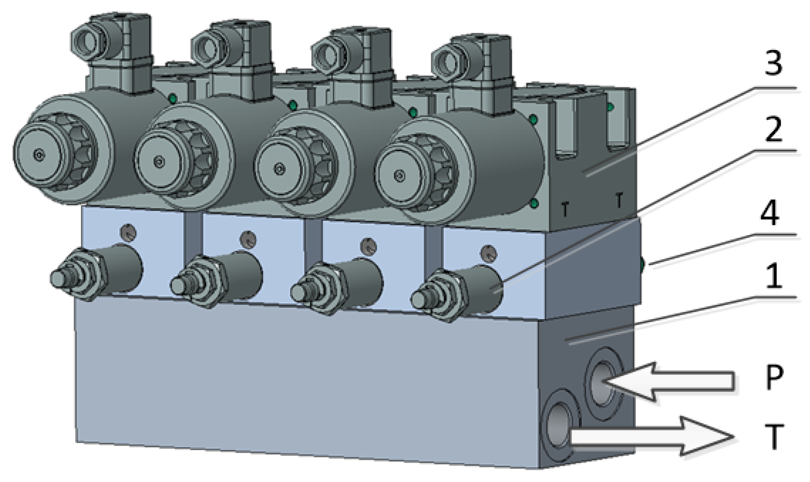
The research object in the form of a grinder valve block is shown in Figure 1.
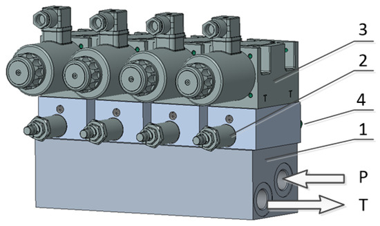
Figure 1.
Scheme of the analyzed valve block: 1—connection plate; 2—flow control valve; 3—electromagnetic control valve; 4—relief valve; P, T—connection ports.
The valve block includes a connection plate (1) that supplies hydraulic oil to multiple parallel-connected flow control valves (2). There are also 4-way, 2-position electromagnetic control valves (3) mounted on the plate, which switch on or off the flow of the working medium to individual hydraulic motors and relief valves (4) that make it easier to stop the engine movement after cutting off the supply of working fluid.
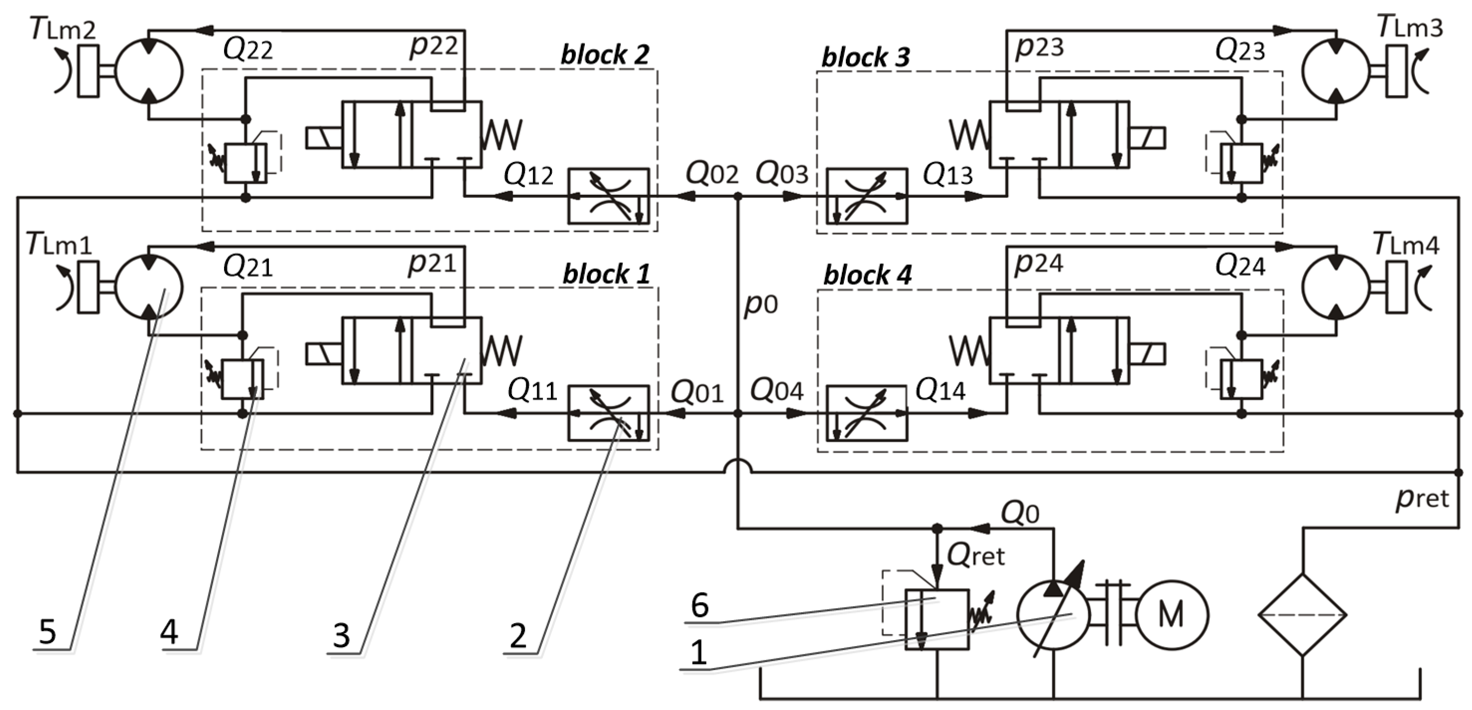
A simplified hydraulic system circuit diagram is shown in Figure 2. A single pump (1) supplies the hydraulic motors (5) to which the grinding disks are attached. The fluid flow is controlled by a block containing flow control valves (2) and electromagnetic valves (3). The grinding wheels rotate at a high speed of more than 5000 rpm. After cutting off the supply flow to the hydraulic motor, it is necessary to enter the braking phase because the high inertia of the grinding disk can keep it rotating for a long time. Therefore, relief valves (4) inhibit motor movement after the flow has been cut off since the resistance moment created by maintaining relatively high pressure in the return line stops rotation effectively. Separate motors may have different load values but must operate approximately at a similar rotational speed. Obtaining the appropriate speed value is ensured by flow control valves, which enable the supply of a proper fluid stream and protect against an excessive increase or decrease in revolutions due to sudden load changes.
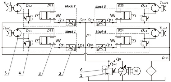
Figure 2.
Hydraulic system diagram: 1—supply unit with a single pump; 2—flow control valve; 3—electromagnetic control valve; 4, 6—relief valve; 5—hydraulic motor.
The main aim of this article is to investigate whether the applied flow control valves can maintain the required speed and compensate for the effects of unfavorable phenomena related to the differentiation of loads imposed on individual motors.
3. Mathematical Model of the System
The mathematical model includes equations describing pressures in lumped volumes, flow rates at specific points and equations of motion of movable elements. The model contains a pump, relief valves, flow control valves, solenoid control valves and hydraulic motors. The input signal is the pump output . A constant value of the flow rate was assumed, taking into account the linear increase in the start-up time and the pulsation characteristic for multi-piston pumps:
where the piston stroke rate per revolution depends on the design parameters of the pump and . For the applied version, it can be written as a function of the control signal :
and the angular speed is maintained constant except the start-up time when it increases linearly:
The mass conservation equation formulated for the supply line has the following form:
The relief valve opens when supply line pressure exceeds the specified value:
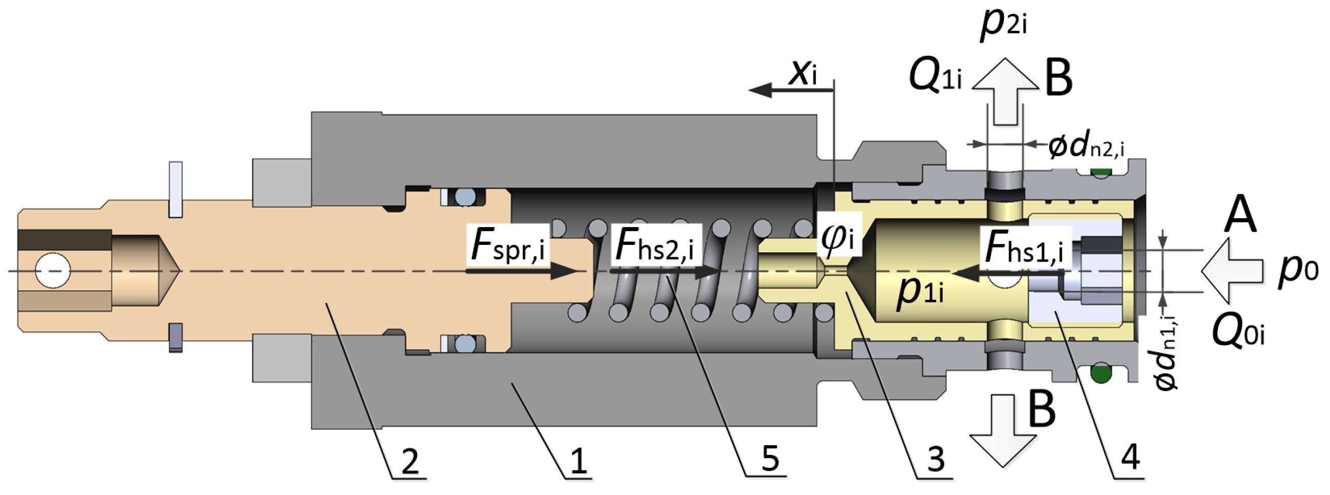
The flow control valve mathematical model was created following the denotations shown in the cross-sectional view (Figure 3).
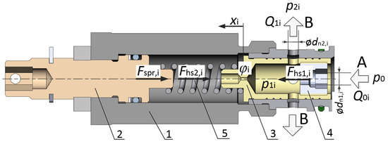
Figure 3.
Cross-sectional view of a flow control valve: 1—body; 2—spring tension adjuster; 3—spool; 4—control insert with a nozzle; 5—spring; A—input; B—output.
The inflow and outflow rates, respectively, and , where is the valve index, may be calculated using the following equations:
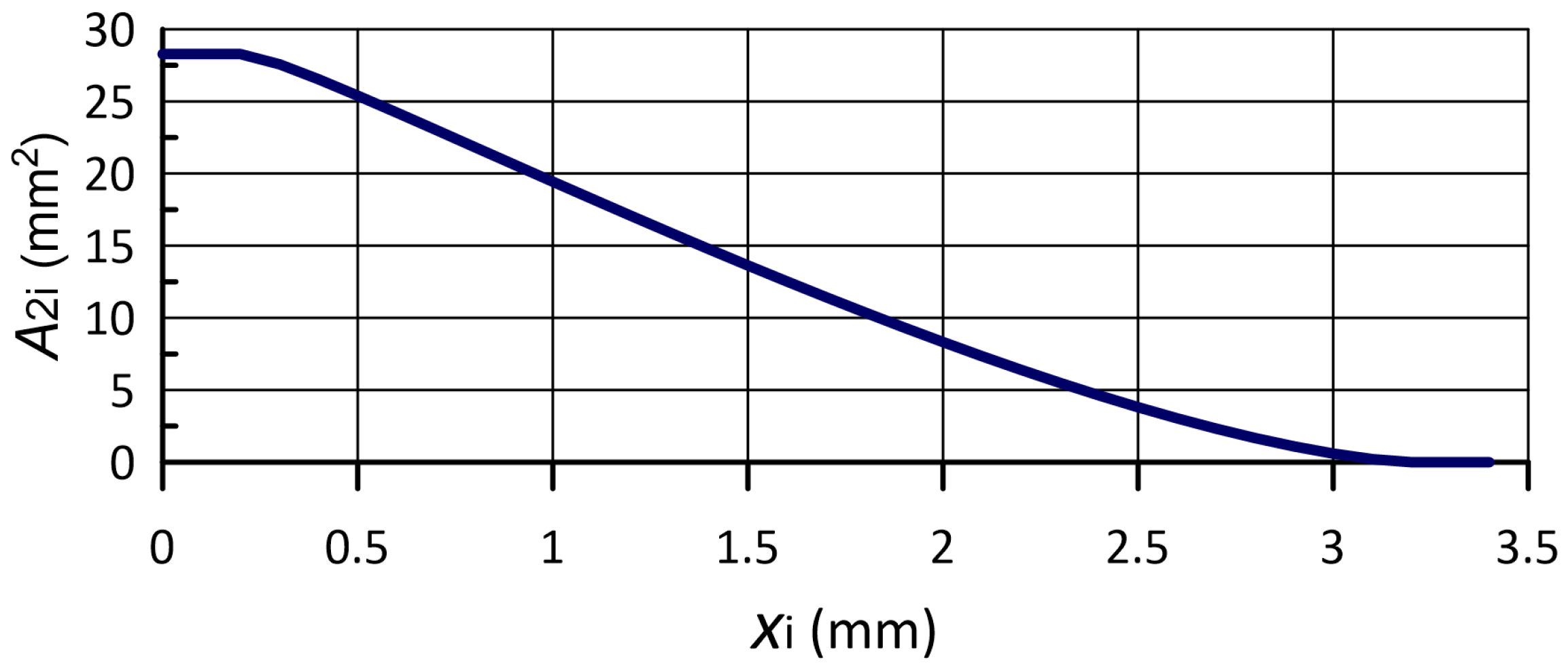
The input nozzle has a fixed area depending on the insert used. For the nominal diameter mm, the nozzle area is mm2. Therefore, the discharge coefficient has also been assumed constant, . On the contrary, the output nozzle area and discharge coefficient depend on the spool position. The nozzle area is shown in Figure 4, while the discharge coefficient is determined in the next section by means of CFD method.

Figure 4.
Output nozzle area of the flow control valve against the spool position.
The equation of the valve spool motion of mass takes into account hydrostatic forces, viscous friction and spring tension force:
The hydrostatic force comes from the pressure difference acting on the front area of the spool: . The viscous friction force is proportional to the fluid viscosity , damping factor and spool velocity: . Spring force includes initial spring tension and deflection due to valve spool displacement: . The required pressure inside the flow control valve can be calculated from the mass conservation equation:
The 2-position directional valves control the inflow of the working medium to individual hydraulic motors based on the control signal:
The hydraulic motor model was created based on a model proposed by Wachholz et al. in [18]. The mass conservation equation is used to determine the pressure inside the motor working chamber based on the input flow rate , rotational speed and the volumetric displacement of the motor :
The motor shaft rotational speed can be calculated concerning resultant moment of inertia , pressure-generated driving torque, load torque and friction torque as a reaction to damping and frictional forces:
where friction torque takes into account Coulomb friction , static friction , Stribeck velocity and viscous friction with the coefficient:
The formulated mathematical model is consistent and complete. It is the base for the simulation model in the following parts of the work.
4. Discrete Model and CFD Analysis
CFD analysis included studies of the flow through the flow control valve, which allowed the discharge coefficient to be determined as a function of spool position. The geometrical valve model was built in PTC Creo, while CFD simulations were carried out using the ANSYS/Fluent university research package.
4.1. Determination of Boundary Conditions and Turbulence Model
The boundary condition at the inlet was the average fluid velocity (velocity specification method: Magnitude, Normal to Boundary). Due to the specificity of the valve operation in the tested system, a fixed flow rate value dm3 min−1 was assigned. The static pressure (outlet condition: Gauge Pressure) with the value of MPa was assumed as the boundary condition at the outlet. The overview of physical parameters used in CFD studies and then in the Simulink model is shown in Table 1.

Table 1.
Physical model parameters.
The estimated value of the Reynolds Number (see Table 1) indicates transient or turbulent flow, depending on the valve spool position. Based on the review of the literature related to CFD studies on hydraulic pumps ([19]) and valves ( [20,21,22,23]), the turbulence model was chosen. Initial tests were performed to select one of the available variants of the model: Standard, Realizable and RNG. As the differences in results obtained with individual variants are negligible, the Standard variant was finally chosen since it required the shortest computation time. In this case, the calculations were approximately 10% and 11% faster than using the Realizable and RNG variants. The chosen turbulence model is based on determining factors such as kinetic energy of the turbulence k, kinetic energy dissipation and turbulent viscosity using the transport equations [24,25,26,27]. The required factors are calculated using the specific model parameters as intensity I, length scale ℓ and constants: , , , and . Table 2 summarizes the parameter values assigned for the flow control valve model taking into account the aforementioned publications and general ANSYS recommendations [28].
Table 2.
Turbulence model parameters.
4.2. Meshing and Mesh Quality Assessment
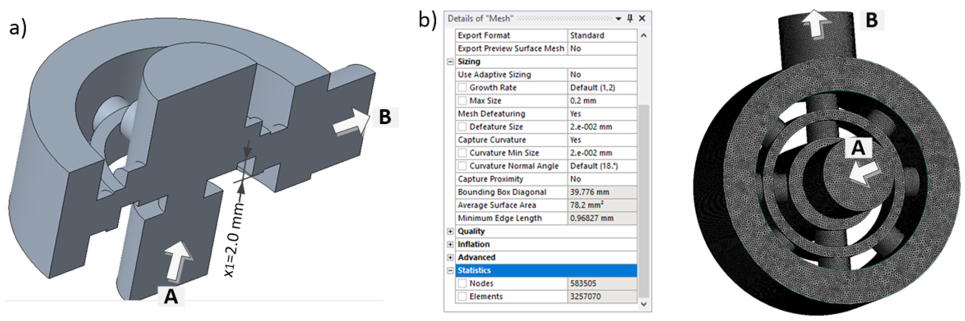
The geometrical fluid model was created in PTC Creo. Then, it was meshed using prism elements at boundary layers and tetrahedrons in the bulk flow. A pressure-based solver was used to achieve the pressure–velocity coupling, taking into account the convergence condition for both mass and momentum residuals. After the initial mesh generation according to ANSYS recommendations, the flow simulation was performed at the fixed flow rate dm3 min−1 and the spool position mm. Subsequent simulations were then performed by applying the progressive mesh refinement technique. As a result, mesh density was increased; however, the computation time was significantly extended. The geometric model in longitudinal section is shown in Figure 5a, while an exemplary mesh (case 3) is shown in Figure 5b. The pressure drop values obtained as a function of the mesh density are summarized in Table 3.
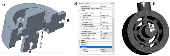
Figure 5.
Flow control valve: (a) cross-sectional view of a geometric model, (b) case 3 of the meshed model.
Table 3.
Mesh quality assessment.
The first mesh refinement caused the resulting pressure drop value to change by % and the second by %. However, further refinement did not change the result significantly, with a considerable extension of the calculation time. Hence, the case 3 model was adopted for further analysis.
4.3. CFD Simulation Results
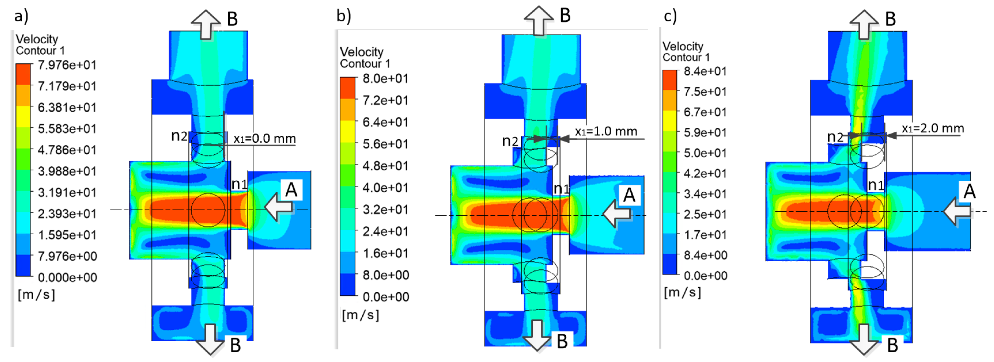
CFD simulations were carried out for the valve spool position mm and the fixed flow rate dm3 min−1. The obtained pressure distributions in the longitudinal cross-section plane for the spool positions mm are shown in Figure 6, while the corresponding velocity distributions are shown in Figure 7, respectively.
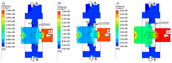
Figure 6.
Pressure distribution depending on the spool position: (a) mm, (b) mm, (c) mm; A—inflow port; B—outflow port; , —nozzles.

Figure 7.
Velocity distribution depending on the spool position: (a) mm, (b) mm, (c) mm; A—inflow port; B—outflow port; , —nozzles.
The given flow rate value with the obtained pressure drop (Table 4) and nozzle area (Figure 4) were used to determine the discharge coefficient of the nozzle, according to the formula:
Table 4.
The nozzle discharge coefficient calculation.
The achieved dependence of the discharge coefficient against the spool position is shown in Figure 8.
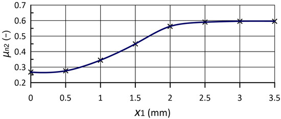
Figure 8.
Discharge coefficient of the output nozzle of the flow control valve against spool position.
5. Modeling and Simulations in Matlab/Simulink
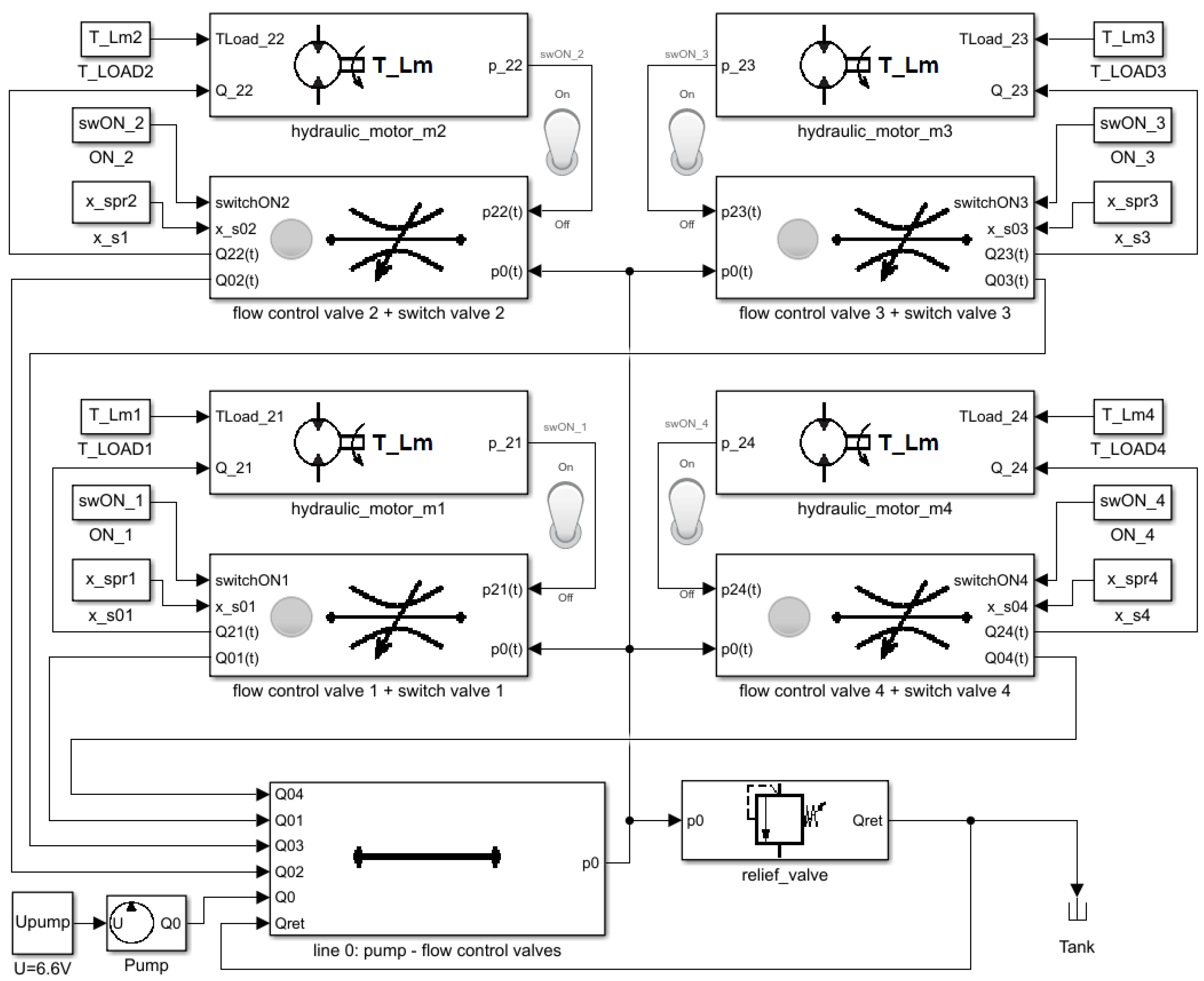
A general view of the hydraulic system model created in Simulink is shown in Figure 9.
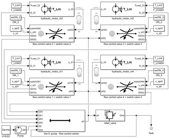
Figure 9.
Simulink model of the hydraulic system.
As seen from the figure, the input signal, in the form of pump output, can be set by the signal. The fluid stream is directed to the supply line () and then divided into four parallel lines, each containing a flow control valve, a switch valve and a hydraulic motor. The working fluid supply to each motor can be opened or shut off by the switching valve using the signal. Each valve can also be assigned an initial spring tension () and a load torque , where .
A crucial component of the flow control valve model is the flow equation through the nozzle, considering variable area and discharge coefficient. A block of this subsystem created for valve index 1 is shown in Figure 10. The input parameters are pressures on both sides of the nozzle and , respectively, and the current spool position . In the bottom part of the diagram, blocks are placed. The blocks are used to determine parameters which depend on the spool position , including the nozzle area and the discharge coefficient .
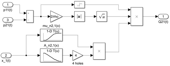
Figure 10.
Simulink model of the nozzle flow equation.
In the first stage, the system operation was simulated with a constant torque load of each hydraulic motor. Next, the feasibility of typical operating cycles was checked. In each case, it was verified that the grinding wheels met the condition of obtaining the minimum rotational speed. Selected parameters of fixed values are presented in Table 5.
Table 5.
Fixed values of simulation model parameters.
5.1. Simulations with Constant Load Torque
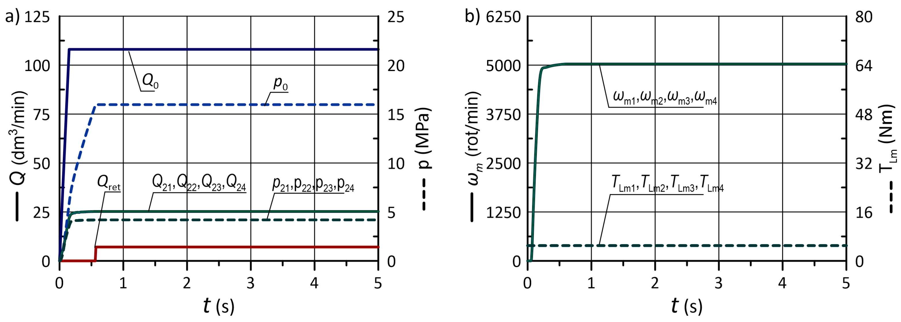
In the first stage, the system operation was analyzed under the condition that all hydraulic motors are loaded with the same torque of a constant value. Taking into account technical parameters of the modeled system components, two load levels were adopted, a low moment value of N m and a high one N m. The obtained results in both cases are shown in Figure 11 and Figure 12, respectively.
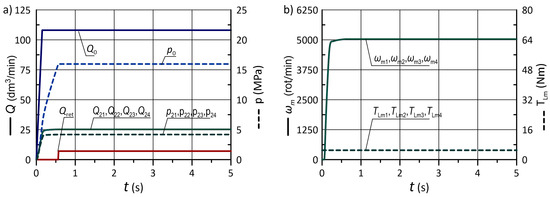
Figure 11.
Results with constant load moment of low value N m: (a) flow rates and pressures; (b) rotational speed of hydraulic motors and load moments.
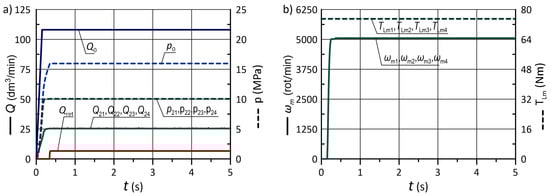
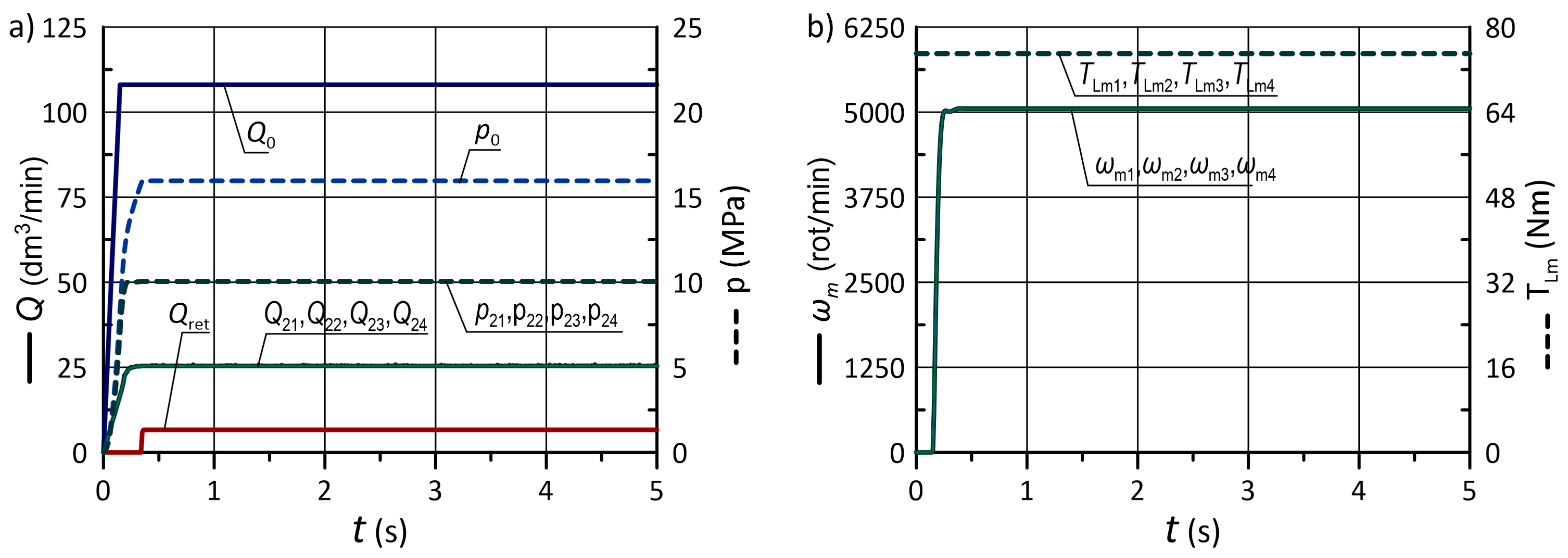
Figure 12.
Results with constant load moment of high value N m: (a) flow rates and pressures; (b) rotational speed of hydraulic motors and load moments.
In each case, the initial tension of springs in all flow control valves was adjusted to obtain the required rotation speed at the given load regarding the valve characteristics: an increase in pressure causes a slight decrease in the flow rate. Pump delivery was set to 108 dm3 min−1, which provides the necessary flow rate to all receivers with a slight surplus. The pressure in the supply line was limited to MPa through a relief valve. This value ensures the sufficiently high driving torque of all hydraulic motors. It should be noted that maintaining the supply line pressure too high leads to significant energy losses.
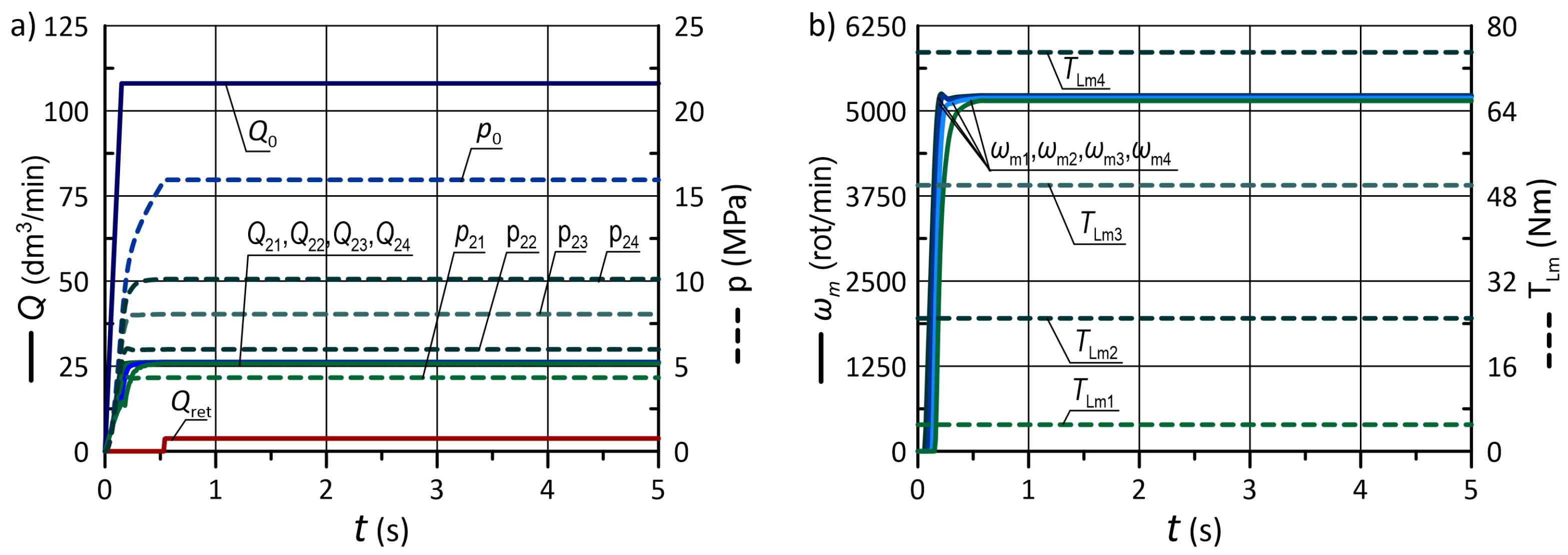
The subsequent test involved loading each hydraulic motor with a different loading moment. The assumed values were N m, N m, N m and N m. The flow rates and pressures in the individual lines of the system are shown in Figure 13a, while the graphs of loading moments and the obtained rotational speeds are demonstrated in Figure 13b, respectively.
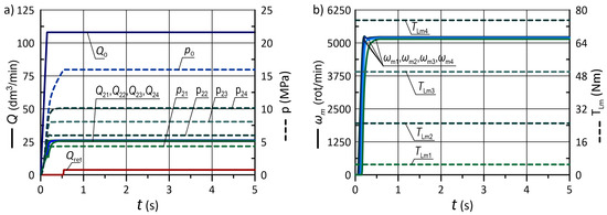
Figure 13.
Results with various loads of individual motors from the range of N m: (a) flow rates and pressures; (b) rotational speed of hydraulic motors and load moments.
To ensure the correct system operation in a wide range of load torques, it was necessary to modify the settings of the valve springs. In particular, the initial tension of all springs, in this case, had to ensure the required flow rate at maximum load. The obtained results show that this causes a slight increase in the rotational speed of the engines with the least load. However, from the view of the system’s proper operation, it is acceptable, particularly since the maximum difference in the rotational speed values does not exceed 5%.
As shown by the analysis carried out at this stage, flow control valves can provide the sufficient flow rate required to obtain the appropriate speed of rotation of the hydraulic motors, regardless of the pressure differences caused by various load torque values.
5.2. Simulations of Typical Operating Cycles
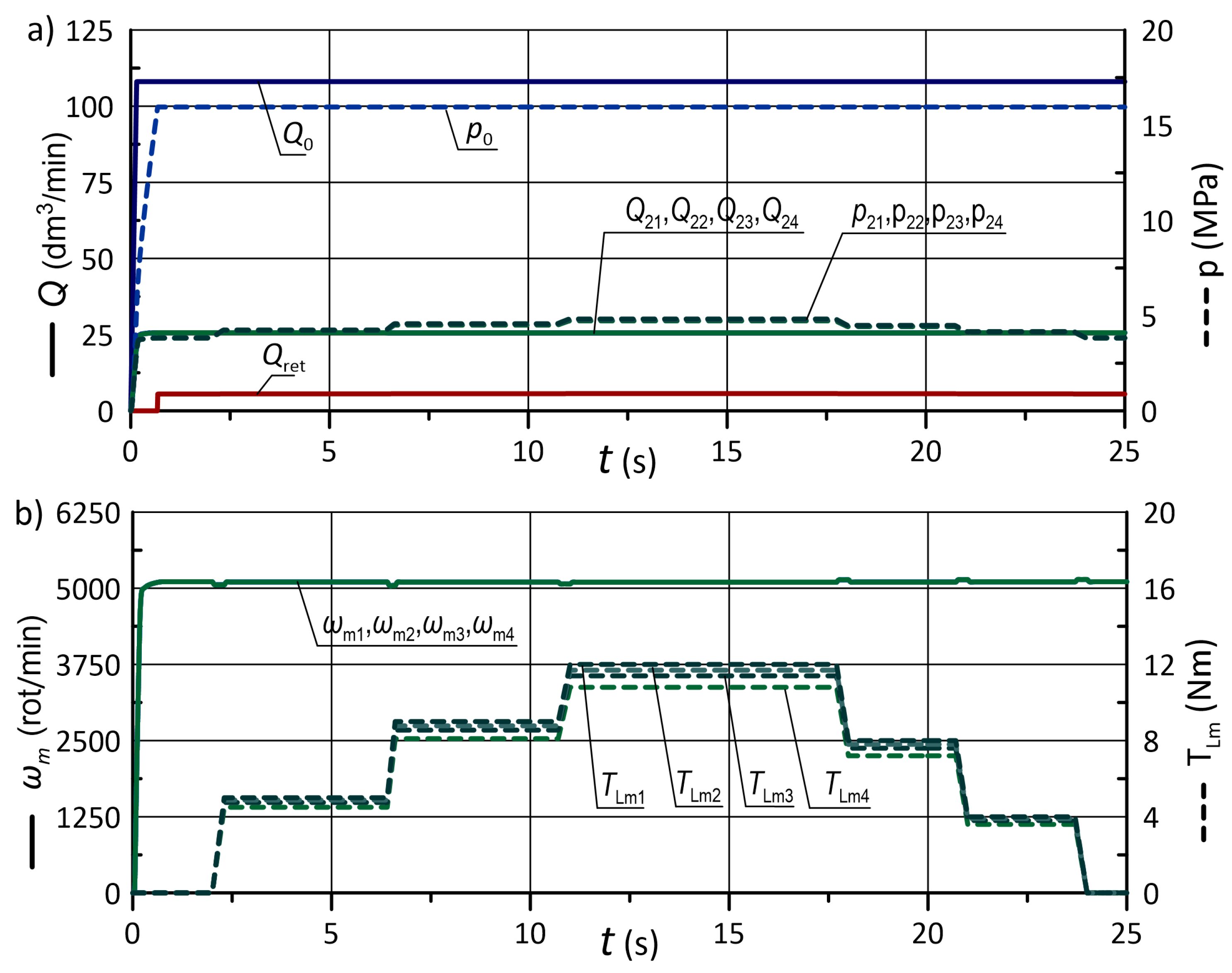
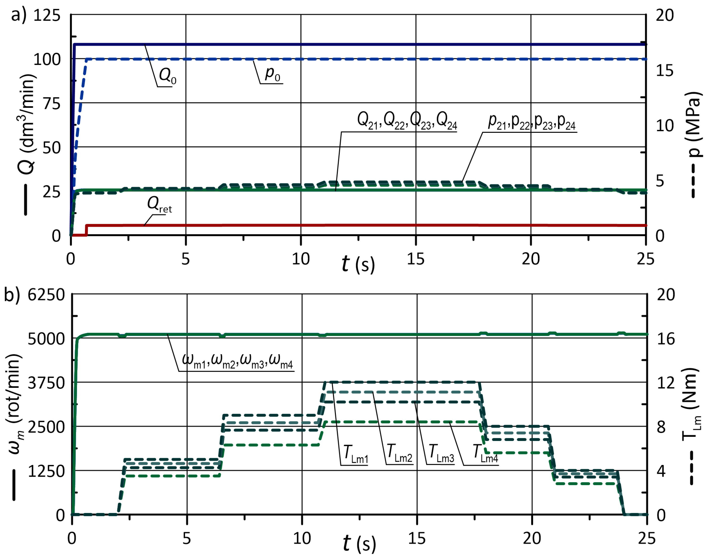
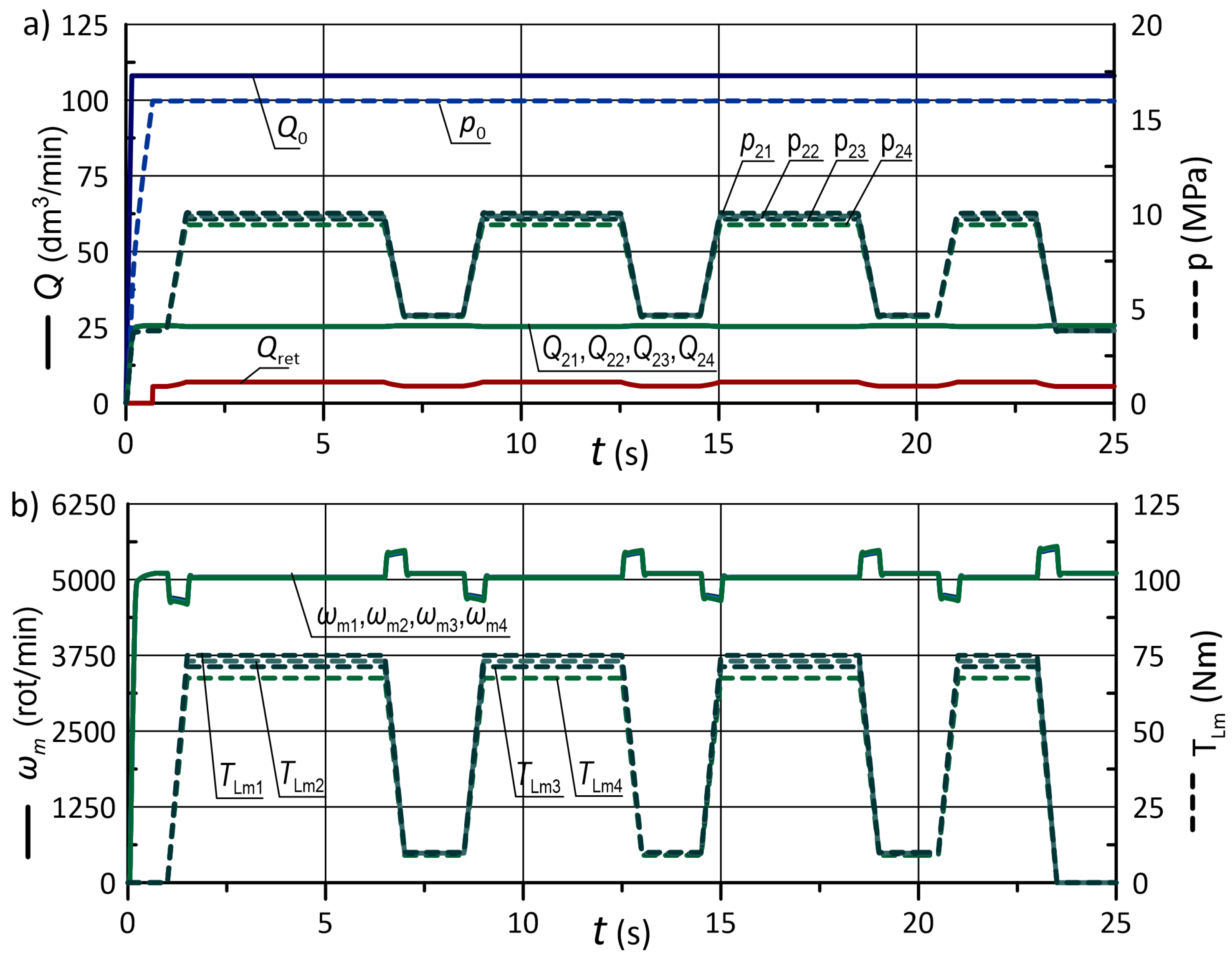
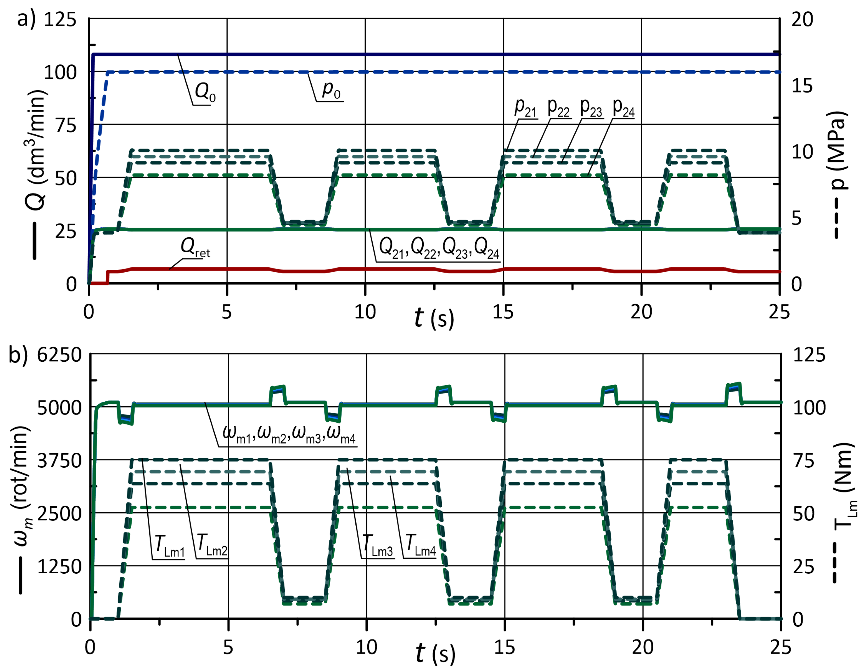
The second stage of the research concerned the feasibility of typical operating cycles. Figure 14 and Figure 15 show the time courses of the parameters as the grinding wheel is gradually pressed against the rail, and then the clamping force is reduced. The maximum load torque is equal to 12 N m and is differentiated for individual hydraulic motors in the range of 10% and 30%, respectively. In turn, Figure 16 and Figure 17 show the cycle of pressing the grinding wheel against the rail several times with a maximum load torque 75 N m. Moreover, in this case, the load moments were differentiated by 10% and 30%, similarly to the previous one.
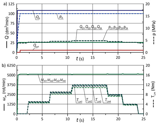
Figure 14.
Operating cycle in a low load range, N m, with load variation of particular motors by 10%; (a) flow rates and pressures; (b) rotational speed of hydraulic motors and load torques.
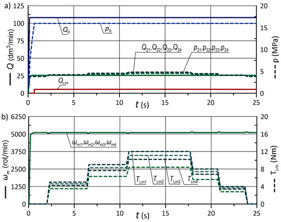
Figure 15.
Operating cycle in a low load range, N m, with load variation of particular motors by 30%; (a) flow rates and pressures; (b) rotational speed of hydraulic motors and load torques.
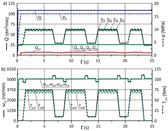
Figure 16.
Operating cycle in a high load range, N m, with load variation of particular motors by 10%; (a) flow rates and pressures; (b) rotational speed of hydraulic motors and load torques.
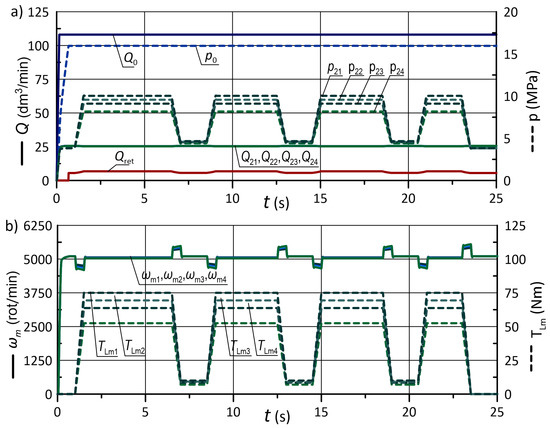
Figure 17.
Operating cycle in a high load range, N m, with load variation of particular motors by 30%; (a) flow rates and pressures; (b) rotational speed of hydraulic motors and load torques.
The obtained results indicate that with significant load changes (70–75 N m) in a short time of 0.2–0.3 s, there is a temporary change in the value of the rotational speed of the motors. As the load torque increases, rotational speed declines down to min. 4750 rot min−1. On the contrary, as the load torque decreases, the rate rises to max. 5330 rot min−1. However, this disturbance does not exceed % and is compensated for by the flow control valve in fewer than s, and therefore does not significantly affect the system operation.
5.3. Discussion of the Results
The results of numerical analyses show that the proposed system allows the required parameters of hydraulic motors to be obtained in the entire load range. Rotational speeds are maintained above minimum values regardless of the loading torque. However, the system’s energy efficiency is also an important issue to consider. For the assumed pressure value on the relief valve MPa, the system requires approximately kW of supply power. The useful power on a single hydraulic motor with a torque load of N m, which generates a pressure of MPa (Figure 11), is kW. This means that the effective power share is %. However, energy efficiency increases if the load is close to the maximum load. In the case of the load of the motors with a moment of N m, the pressure is MPa (Figure 12), and the useful power kW. The effective power share in this case is %.
6. Summary and Conclusions
The article concerns the numerical analysis of a hydraulic system in which it is necessary to divide the stream of working fluid into multiple receivers connected in parallel on the example of a rail grinder. This issue is crucial from a practical point of view because it reduces the device’s total cost by simplifying the hydraulic supply system and not requiring advanced electronic control systems. The analyzed system included a hydraulic supply unit containing a variable displacement pump and a relief valve which supplied four operating lines connected in parallel. Each line consisted of a flow control valve, a switch valve, a hydraulic motor and a relief valve. The motors were loaded with an external torque of a constant or variable value. The system was designed to work with the nominal pressure in the supply line MPa and the flow rate through each of the receivers dm3 min−1. In the first stage, a geometric model of the flow control valve was built, and tests were carried out to obtain pressure and velocity distributions and calculate the discharge coefficient. Then, a mathematical model of the whole hydraulic system was formulated. Based on the CFD results and the mathematical model, a simulation model was built in the Matlab/Simulink environment. Numerical analyses were carried out, which showed that the proposed solution ensures the maintenance of appropriate operating parameters, regardless of the value and course of the load torque. Detailed conclusions:
- The proposed solution can be used in practice in systems with the requirement to keep the controlled parameter above the threshold value. This work concerned, in particular, the maintenance of the minimum flow rate, and thus required rotational speed of hydraulic motors regardless of the load;
- The applied hydraulic components do not require an electric power supply, which is especially important under the track grinder working conditions: continuous movement, high temperatures in the grinding area and the influence of weather conditions;
- The flow rate settings can be adjusted to a small extent by modifying the initial tension of the valve spring . The settings can be changed in a broader range by using a valve spring with a different stiffness . Finally, valves of larger or smaller nominal sizes can also be used;
- It is essential to pre-define a load torque range and adapt the relief valve settings to minimize energy loss during the implementation of operating cycles. The highest energy efficiency achieved when working under a load close to the maximum was approximately 80%. However, with a low load of about 10% of the allowable value, the energy efficiency drops to 30%.
Author Contributions
Conceptualization, E.L.; methodology, G.F.; software, E.L. and G.F.; validation, E.L.; formal analysis, E.L.; investigation, E.L. and G.F.; resources, E.L.; writing—original draft preparation, G.F.; writing—review and editing, G.F. and E.L.; visualization, G.F.; supervision, E.L.; project administration, G.F.; funding acquisition, E.L. and G.F. All authors have read and agreed to the published version of the manuscript.
Funding
This research received no external funding.
Institutional Review Board Statement
Not applicable.
Informed Consent Statement
Not applicable.
Data Availability Statement
Not applicable.
Conflicts of Interest
The authors declare no conflict of interest.
Nomenclature
| Indices | |
| 0 | supply line |
| i, where | flow control valve and hydraulic motor index |
| m | hydraulic motor |
| return line | |
| v | flow control valve |
| Parameters | |
| , | flow control valve , nozzle area, spool area (m2) |
| fluid bulk modulus (Pa) | |
| turbulence model constants (-) | |
| design parameters of a hydraulic motor (-) | |
| force acting on spool: hydrostatic 1, 2, spring, viscous friction (N) | |
| turbulence model factors: intensity, length scale (-, m) | |
| hydraulic motor shaft + grinding wheel moment of inertia (kg m2) | |
| , | supply power, useful power on the i-th motor (kW) |
| , | flow rate: pump, return line (dm3 min−1) |
| , | flow rate: inlet and outlet of flow control valve (dm3 min−1) |
| flow rate at inlet to hydraulic motor (dm3 min−1) | |
| , , | motor friction torque, Coulomb torque, static torque (N m) |
| torque load of the motor (N m) | |
| pump control signal (V) | |
| volume: supply line, inside flow control valves, motor lines (m3) | |
| valve spring stiffness (N m−1) | |
| valve spool mass (kg) | |
| pressure: supply line, return line (MPa) | |
| pressure: inside flow control valve, hydraulic motor line (MPa) | |
| , | pump piston stroke rate/max. stroke rate per revolution (m3 rev−1) |
| turbulence model constants (-) | |
| time, start-up time (s) | |
| valve spool position (m) | |
| initial tension of valve spring (m) | |
| z | number of pump pistons (-) |
| pressure drop at valve nozzle (MPa) | |
| effective power share (%) | |
| fluid dynamic viscosity (Pa s) | |
| fluid kinematic viscosity (m2 s−1) | |
| , | discharge coefficient of flow control valve nozzles (-) |
| turbulent viscosity (m2 s−1) | |
| fluid density (kg m−3) | |
| flow control valve spool damping coefficient (N s m−1) | |
| hydraulic motor damping factor (m) | |
| pump rotational speed, pump nominal speed (rev s−1) | |
| , | motor rotational speed, motor Stribeck velocity (rev s−1) |
References
- Bekele, T.; Åman, R.; Handroos, H. The Control of Multiple Actuators using Single IEHEC Pump/Motor. In Proceedings of the 10th International Fluid Power Conference Dresden (10. IFK), Dresden, Germany, 8–10 March 2016; pp. 73–88. [Google Scholar]
- Yao, J.; Wang, P.; Yin, Y.; Li, M.; Li, Y. Power management of multi-source network hydraulic system with multiple actuators. Energy Convers. Manag. 2020, 223, 113247. [Google Scholar] [CrossRef]
- Lisowski, E.; Filo, G. Analysis of a proportional control valve flow coefficient with the usage of a CFD method. Flow Meas. Instrum. 2017, 53, 269–278. [Google Scholar] [CrossRef]
- Guo, Q.; Chen, Z.; Shi, Y.; Yan, Y.; Guo, F. Synchronous control of multiple electrohydraulic actuators under distributed switching topologies with lumped uncertainty. J. Frankl. Inst. 2022, 359, 4288–4306. [Google Scholar] [CrossRef]
- Guo, Q.; Chen, Z.; Shi, Y.; Li, X.; Yan, Y.; Guo, F.; Li, S. Synchronous control for multiple electrohydraulic actuators with feedback linearization. Mech. Syst. Signal Process. 2022, 178, 109280. [Google Scholar] [CrossRef]
- Lei, T.; Wang, J.; Yao, Z. Modelling and Stability Analysis of Articulated Vehicles. Appl. Sci. 2021, 11, 3663. [Google Scholar] [CrossRef]
- Han, J.; Wang, F.; Wang, Y. A Control Method for the Differential Steering of Tracked Vehicles Driven Independently by a Dual Hydraulic Motor. Appl. Sci. 2022, 12, 6355. [Google Scholar] [CrossRef]
- Huang, J.; Wang, X.; Wang, H.; Hao, H. Development of a flow control valve with digital flow compensator. Flow Meas. Instrum. 2019, 66, 157–169. [Google Scholar] [CrossRef]
- Okhotnikov, I.; Noroozi, S.; Sewell, P.; Godfrey, P. Evaluation of steady flow torques and pressure losses in a rotary flow control valve by means of computational fluid dynamics. Int. J. Heat Fluid Flow 2017, 64, 89–102. [Google Scholar] [CrossRef]
- Lisowski, E.; Filo, G. CFD analysis of the characteristics of a proportional flow control valve with an innovative opening shape. Energy Convers. Manag. 2016, 123, 15–28. [Google Scholar] [CrossRef]
- Kumar, S.; Tewari, V.K.; Bharti, C.K.; Ranjan, A. Modeling, simulation and experimental validation of flow rate of electro-hydraulic hitch control valve of agricultural tractor. Flow Meas. Instrum. 2021, 82, 102070. [Google Scholar] [CrossRef]
- Adeoye, A.; Aderoba, A.; Oladapo, B. Simulated Design of a Flow Control Valve for Stroke Speed Adjustment of Hydraulic Power of Robotic Lifting Device. Procedia Eng. 2017, 173, 1499–1506. [Google Scholar] [CrossRef]
- Sun, X.; Wang, Y.; Zhang, J.; Lei, F.; Zhao, D.; Hong, H. Multi-Objective Optimization Design of Key Parameters of a Stepless Flow Control System with Multi-System Coupling Characteristics. Appl. Sci. 2022, 12, 1301. [Google Scholar] [CrossRef]
- Wang, Y.; Liu, X.; Chen, J.; Chen, W.; Li, C.; Huo, D. Design and control performance optimization of dual-mode hydraulic steering system for wheel loader. Autom. Constr. 2022, 143, 104539. [Google Scholar] [CrossRef]
- Leephakpreeda, T. Flow-sensorless control valve: Neural computing approach. Flow Meas. Instrum. 2003, 14, 261–266. [Google Scholar] [CrossRef]
- Zhang, J.; Wang, D.; Xu, B.; Su, Q.; Lu, Z.; Wang, W. Flow control of a proportional directional valve without the flow meter. Flow Meas. Instrum. 2019, 67, 131–141. [Google Scholar] [CrossRef]
- Feng, H.; Song, Q.; Ma, S.; Ma, W.; Yin, C.; Cao, D.; Yu, H. A new adaptive sliding mode controller based on the RBF neural network for an electro-hydraulic servo system. ISA Trans. 2022, 129, 472–484. [Google Scholar] [CrossRef]
- Wachholz, L.; Valdiero, A.; Rasia, L. Mathematical modeling of a hydraulic motor operated and controlled by proportional valve. In Proceedings of the 25th ABCM International Congress of Mechanical Engineering, Uberlandia, Brazil, 20–25 October 2019. [Google Scholar] [CrossRef]
- Anh, P.N.; Bae, J.S.; Hwang, J.H. Computational Fluid Dynamic Analysis of Flow Rate Performance of a Small Piezoelectric-Hydraulic Pump. Appl. Sci. 2021, 11, 4888. [Google Scholar] [CrossRef]
- Jin-yuan, Q.; Lin, W.; Zhi-jiang, J.; Jian-kai, W.; Han, Z.; An-le, L. CFD analysis on the dynamic flow characteristics of the pilot-control globe valve. Energy Convers. Manag. 2014, 87, 220–226. [Google Scholar] [CrossRef]
- Domagała, M.; Momeni, H.; Fabiś-Domagała, J.; Saeed, B.; Filo, G.; Amzin, S. Fluid-Structure Interaction Simulation of Flow Control Valve. Mater. Res. Proc. 2020, 17, 036042. [Google Scholar] [CrossRef]
- Wen, Q.; Liu, Y.; Chen, Z.; Wang, W. Numerical simulation and experimental validation of flow characteristics for a butterfly check valve in small modular reactor. Nucl. Eng. Des. 2022, 391, 111732. [Google Scholar] [CrossRef]
- Domagała, M.; Momeni, H.; Fabiś-Domagała, J. The Influence of Oil Contamination on Flow Control Valve Operation. Mater. Res. Proc. 2022, 24, 001008. [Google Scholar] [CrossRef]
- Lisowski, E.; Filo, G.; Rajda, J. Pressure compensation using flow forces in a multi-section proportional directional control valve. Energy Convers. Manag. 2015, 103, 1052–1064. [Google Scholar] [CrossRef]
- Chen, F.; Qian, J.; Chen, M.; Zhang, M.; Chen, L.; Jin, Z. Turbulent compressible flow analysis on multi-stage high pressure reducing valve. Flow Meas. Instrum. 2018, 61, 26–37. [Google Scholar] [CrossRef]
- Scuro, N.; Angelo, E.; Angelo, G.; Andrade, D. A CFD analysis of the flow dynamics of a directly-operated safety relief valve. Nucl. Eng. Des. 2018, 328, 321–332. [Google Scholar] [CrossRef]
- Filo, G.; Lisowski, E.; Rajda, J. Design and Flow Analysis of an Adjustable Check Valve by Means of CFD Method. Energies 2021, 14, 2237. [Google Scholar] [CrossRef]
- ANSYS Fluent in ANSYS Workbench User’s Guide, 1st ed.; ANSYS Inc.: Canonsburg, PA, USA, 2020; Available online: http://www.ansys.com (accessed on 19 September 2022).


Publisher’s Note: MDPI stays neutral with regard to jurisdictional claims in published maps and institutional affiliations. |
© 2022 by the authors. Licensee MDPI, Basel, Switzerland. This article is an open access article distributed under the terms and conditions of the Creative Commons Attribution (CC BY) license (https://creativecommons.org/licenses/by/4.0/).