Discontinuity Recognition and Information Extraction of High and Steep Cliff Rock Mass Based on Multi-Source Data Fusion

Abstract

It is fundamental to acquire accurate point cloud information on rock discontinuities efficiently and comprehensively when evaluating the stability of rock masses. Taking a high and steep cliff as an example, we combined 3D laser scanning and UAV photogrammetry technology to collect rock data, and proposed an intelligent identification method for rock discontinuities based on the multi-source fusion of point clouds. First, the 3D-laser-collected point cloud data were used as the basis to fuse with the UAV-photogrammetry-collected data, and the unified coordinate system and improved ICP algorithm were used to obtain the complete 3D point cloud in the study area. Secondly, we used neighborhood information entropy to achieve adaptive neighborhood-scale selection and to obtain the optimal neighborhood radius for the KNN search, to effectively calculate the point cloud normal vector and rock mass orientation information. Finally, the KDE algorithm and DBSCAN algorithm were combined for rock discontinuity clustering to achieve intelligent identification and information extraction of the rock structural plane. The clustering results were imported into the DSE program developed based on Matlab to calculate the discontinuity spacing and continuity of the rock mass structure, and to efficiently obtain the parameters of rock mass occurrence. The research results showed that this method can effectively solve the problem of incomplete-data-acquisition ground 3D laser scanning in complex geological conditions, and UAV photogrammetry prone to blurred images in depressed areas. When the extraction results were compared with the field-measured rock occurrence, the average dip angle error was about 2°, the average dip direction error was 1°, and the recognition results met the accuracy requirements. The research results provide a feasible scheme for the identification and extraction of discontinuities of high and steep rock masses.

1. Introduction

In rock mass structures, rock discontinuities occupy an extremely important position. Currently, the most commonly used method for investigating rock discontinuities is to use the geological compass and tape measure to obtain the orientation information of geological rock discontinuities, including tendency, dip angle, dip direction, spacing, density, and roughness. This method is simple with accurate results, but it is only applicable to measuring simple rock discontinuity surfaces that can be directly contacted, and its applicable scenarios are limited [1]. With the development of surveying technology, noncontact measurement are gradually being applied in geological surveys, such as photogrammetry [2,3], 3D laser scanning technology [4,5,6], and underground television [7]. Among them, 3D laser scanning and UAV photogrammetry can obtain rock mass point cloud information quickly and accurately. Based on the obtained point cloud, K-means clustering [8], region growing [9], the Hough normal vector, and HSV [10] are used to process the point cloud, which can further achieve the intelligent identification of rock mass discontinuities, to dig out their detailed information such as spacing and roughness. Therefore, it has been favored by scholars.

Some scholars have even made innovations in rock structural surface extraction algorithms. For example, Ge et al. [11] used an improved region growing algorithm and analytic geometry theory to construct a 3D model of a point cloud and intelligently identify the rock mass orientation information. Chen et al. [12] used the 3D laser scanning technology to obtain the rock mass point cloud information and intelligently identify the rock mass discontinuities by the improved Ransac algorithm and Graham Scan algorithm. Zhang et al. [13] used a double-nested mean-shift clustering algorithm and a region growing algorithm to identify and classify rock discontinuity surfaces to obtain geological information. Wang et al. [14] proposed a rock mass discontinuity identification algorithm based on the sensitivity parameters (K-nearest-neighbor points, pinch angle threshold j, and filtering factor f) to rapidly identify rock mass discontinuities in the 3D point clouds. Chen et al. [15] achieved the automatic identification of information of rock mass discontinuities based on the 3D point cloud data of the rock mass surface, through four steps of structural grouping analysis, grouping optimization, structural fitting, and coordinate system conversion. The reliability and accuracy of this method were verified by comparing with the field survey results of the slope rock discontinuities on the slope surface, which provided a reference method for the extraction of geometric information of rock discontinuities in 3D point clouds.

In summary, using 3D laser scanning and photogrammetry is currently the most effective way to obtain a rock mass point cloud in the shortest time, but for special geographic situations, there are the following problems: first, when facing complex terrain, it is difficult to obtain complete point cloud information of rock masses by a single measurement method; second, when using different technical means to obtain multi-source point cloud data of rock masses, it is uncertain how to carry out multi-source point cloud fusion to ensure data integrity on the premise of data quality; finally, based on the multi-source point cloud information, how to accurately and quickly obtain the occurrence information of the rock mass is the focus and difficulty of the research, but there is very limited research in this area.

Therefore, this paper takes a high and steep cliff on the south side of Laojun Peak in Huidong County, Sichuan Province as an example, and uses 3D laser scanning and UAV photogrammetry to collect data. Based on the multi-source fusion point cloud, the improved nearest-neighbor search algorithm combined with the coplanarity criterion is used to calculate the point cloud normal vector and HSV color rendering. Meanwhile, the rock discontinuities are clustered by combining the kernel density estimation and the density-based clustering algorithm, to intelligently identify the rock discontinuities. The accuracy of this method is verified by comparing and analyzing with the field survey results.

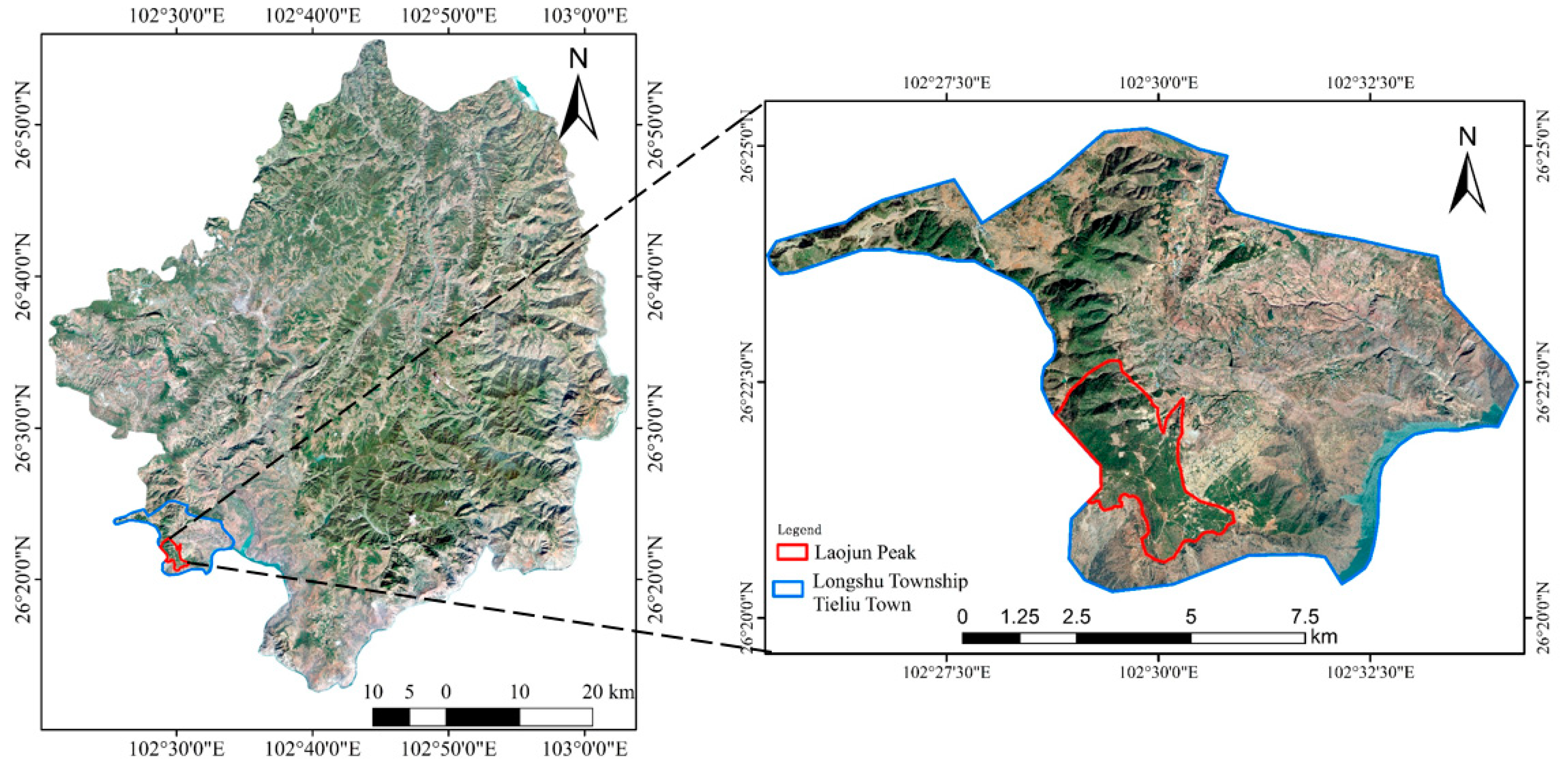
2. Study Area

Laojun Peak Tourist Scenic Area, in Tieliu Town, Huidong County, Liangshan Prefecture of Sichuan Province, sits in the hinterland of Jinsha River Grand Canyon, about 2000 m above sea level. It has formed a majestic and magnificent natural landscape with a long-standing history, which is entitled as “the first peak in southern Ba Shu”, as shown in Figure 1. Since the completion of the national Wudongde Power Station, the water level of Jinsha River Canyon in Huidong County has risen, making the scenery more charming with a higher tourism value. In order to improve the tourism infrastructure, a tourist resort hotel needs to be built at the top of Laojun Peak, and a glass walkway needs to be paved. Therefore, considering its safety and project feasibility, rock structure analysis is required to provide baseline data for rock stability evaluation.

Our study area is located in the scenic area of Laojun Peak, with geographical coordinates ranging from 102°31′1.61″ to 102°31′14.74″ east longitude and 26°20′54.14″ to 26°21′1.86″ north latitude. The overall geomorphology is located at the intersection of two major geomorphological units, the southern edge of the western Sichuan Plateau and the northern side of the Yunnan-Guizhou Plateau, featured mainly by the Zhongshan terrain. The terrain is generally high in the east and low in the west, and the mountains are mostly distributed in a north–south direction. The two banks are steep canyon terrain, with rapid water flow and dangerous beaches. The elevation of the valley bottom is 692–892 m, and the cutting depth is 1000~3000 m, which is the lowest erosion datum. According to the geological data, the geomorphological type in this region can be divided into four types according to their origins: eroded tectonic mesas, dissolution tectonic mesas, denudation tectonic low mesas, and tectonic erosion accumulation, which are shown in Figure 2.

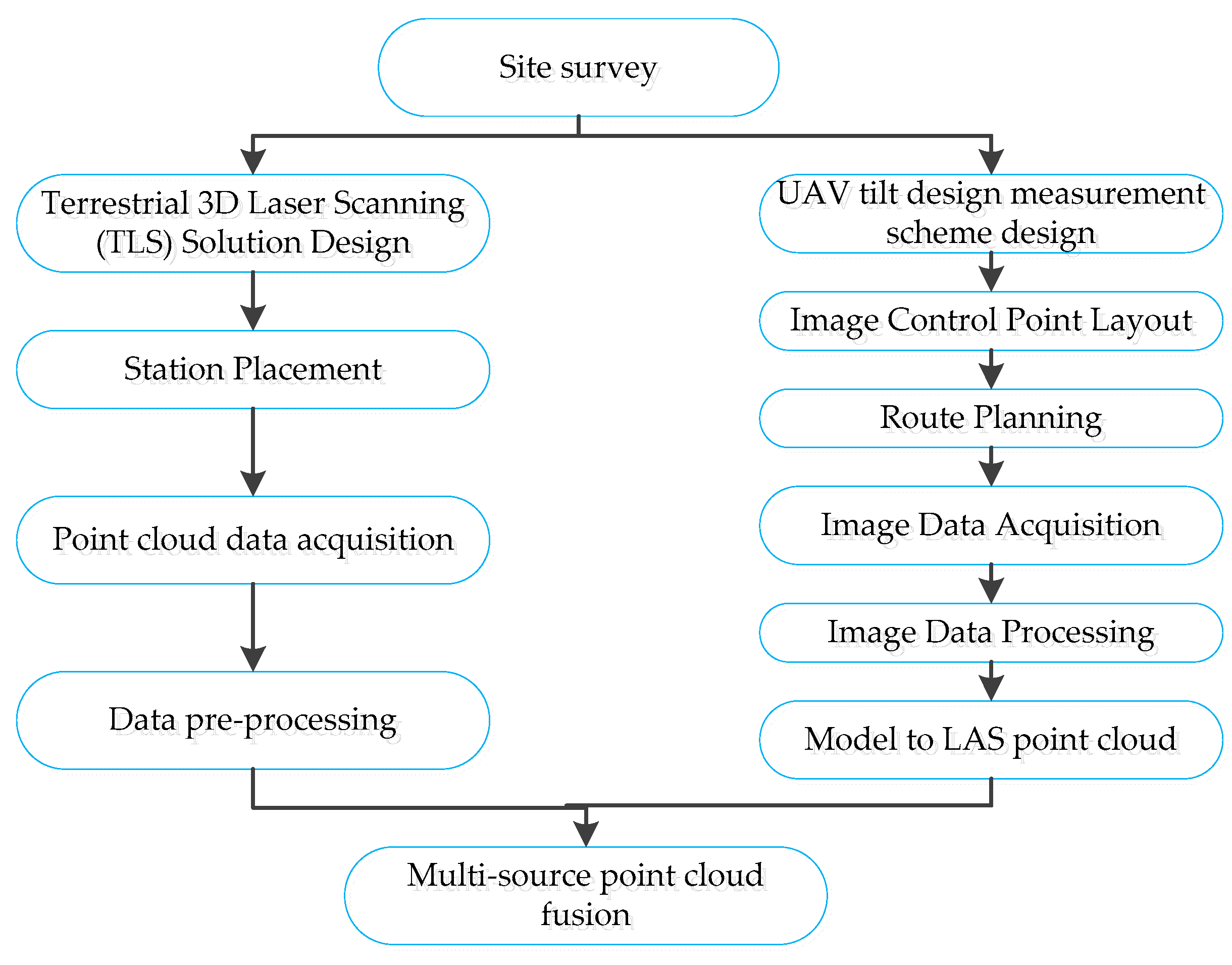
3. Data Acquisition and Processing

Due to the large difference in height of steep cliffs, which is close to 200 m, it is difficult to obtain complete point cloud information by a single technical means. We, therefore, adopted an integrated ground-air approach to acquire the point cloud data. In this paper, the ground 3D laser scanning point cloud data were mainly used with high accuracy, and the point cloud data from UAV tilt photogrammetry were also collected to supplement. Then, we performed data fusion of the two point clouds to achieve mutual complementation of different data sources and to ensure their integrity. The fused point cloud data can fully reflect the terrain features. The process of point cloud acquisition is shown in Figure 3.

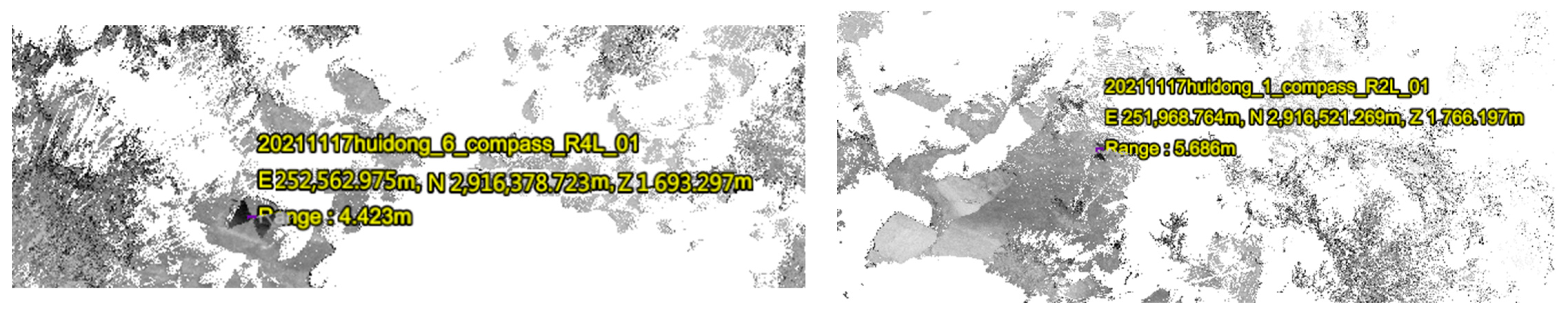
3.1. Ground 3D Laser Scanning Point Cloud Data and Pre-Processing

The Maptek I-site 8200ER ground 3D laser scanner with IP65 protection class was used for scanning, and the main parameters are shown in

Table 1. Parameters of Maptek I-site 8200ER ground 3D laser scanner.

Parameter Types	Parameter Indicators
Instrument leveling/(″)	20″ (Built-in compensator)
Compass/(°)	±1
Maximum measuring range/(m)	500
Minimum measurement range/(m)	1
Distance accuracy/(mm)	6
Scanning Range/(m)	Vertical 270°, horizontal 360°
Angular Resolution/(°)	0.2–0.025

. I horizontal angle and vertical angle were measured by a test accuracy of 7″ [16].

The free station setting was adopted to ensure that the data from multiple stations were in the same coordinate system. In order to obtain a complete point cloud and ensure a 30% overlap of the scanned area, data acquisition could only be carried out by multiple stations. At the same time, GNSS RTK was used on-site to measure the 3D coordinates of the target points. In total, 7 stations were set-up to scan over 17.48 million point clouds, and the scanning area is shown in Figure 4a,b.

In the data acquisition process, as the coordinate system of each survey site cloud data point is independent of each other, and the acquisition process will inevitably generate noise points, the point cloud must be pre-processed before processing and analysis. By using the supporting software Maptek I-Site Studio to perform stitching, alignment, denoising, and other operations, the point cloud data of the study area were obtained, as shown in Figure 4c,d. The 3D laser scanning technology had a high measurement accuracy and high speed, but the scanning range was limited in the vertical direction, and some point clouds had voids when facing complex terrain conditions such as high and steep cliffs (Figure 5).

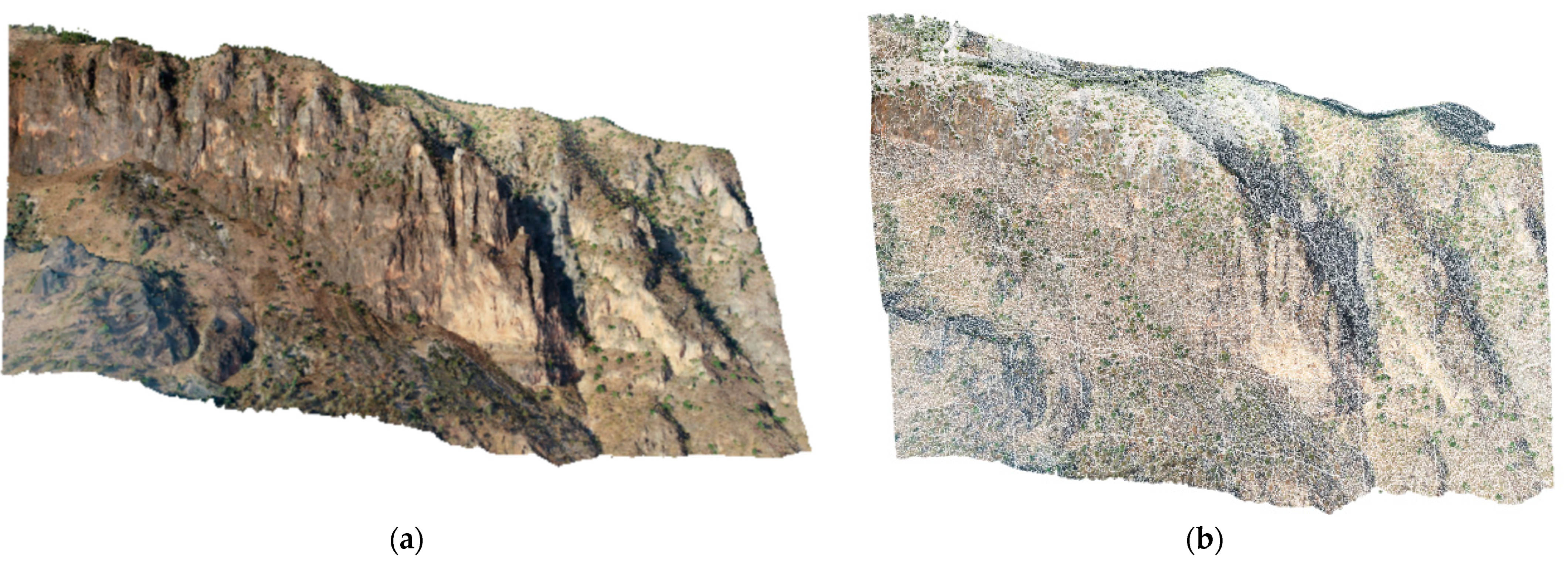
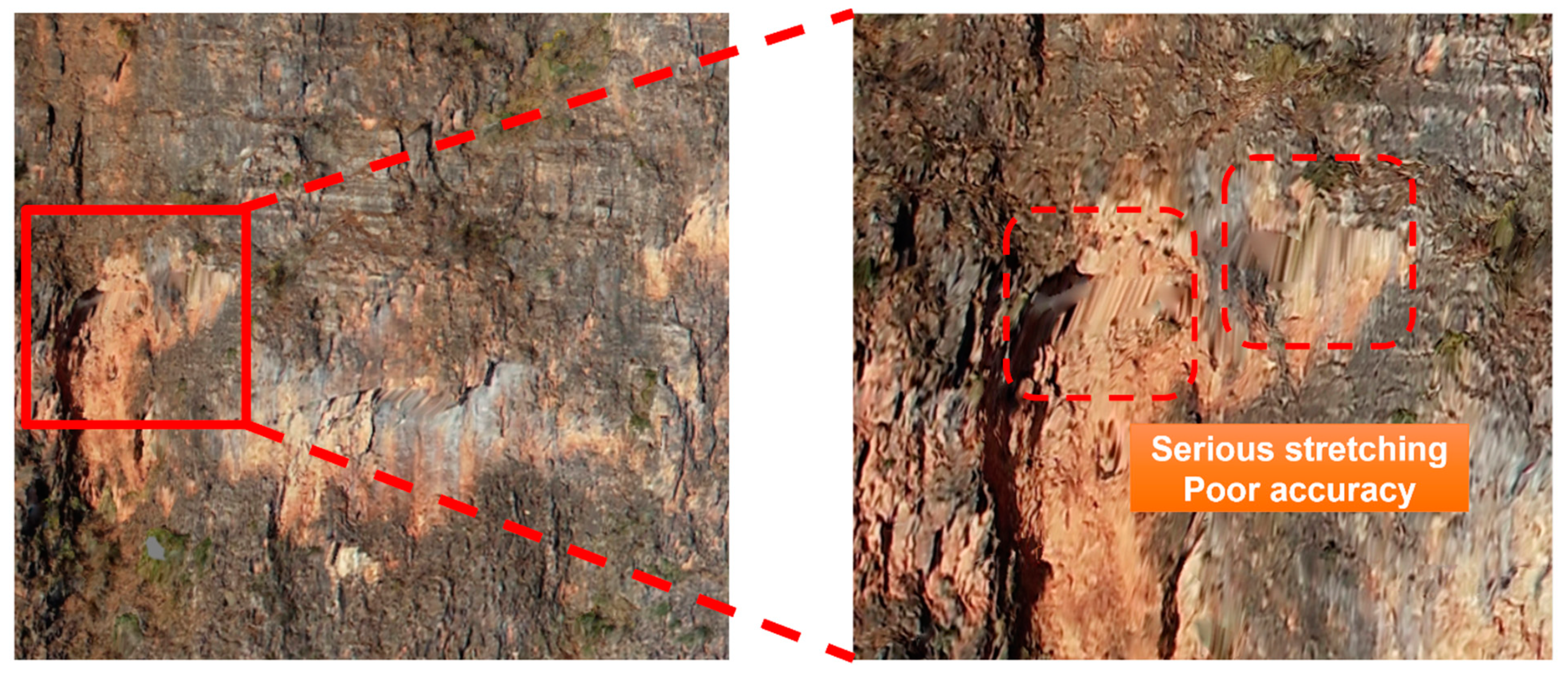
3.2. UAV Photogrammetry Data Acquisition and Pre-Processing

The data were collected using a DJI Genie 4 Pro 20-megapixel drone, but due to the high altitude difference and wind direction and speed, a manual flight mode was used and the number of aerials collected was 1204. The data processing was performed by ContextCapture Center software for processing operations such as image element point judging and aerial triangulation to obtain the rock LAS point cloud and 3D model, as shown in Figure 6. However, in the manual flight mode, due to the aerial film camera focusing on the center of the aerial film, which will cause serious distortion of the photos of the high and steep cliff at the bottom, we could not acquire a precise measurement of the steep cliff at the bottom (Figure 7). For this, point cloud fusion was needed.

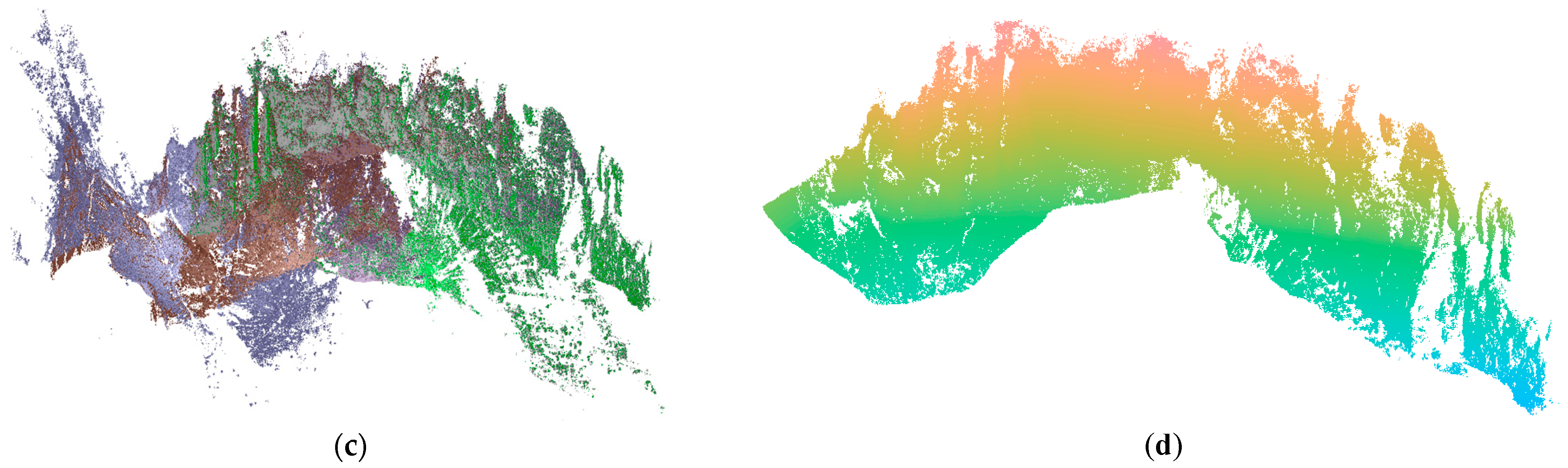
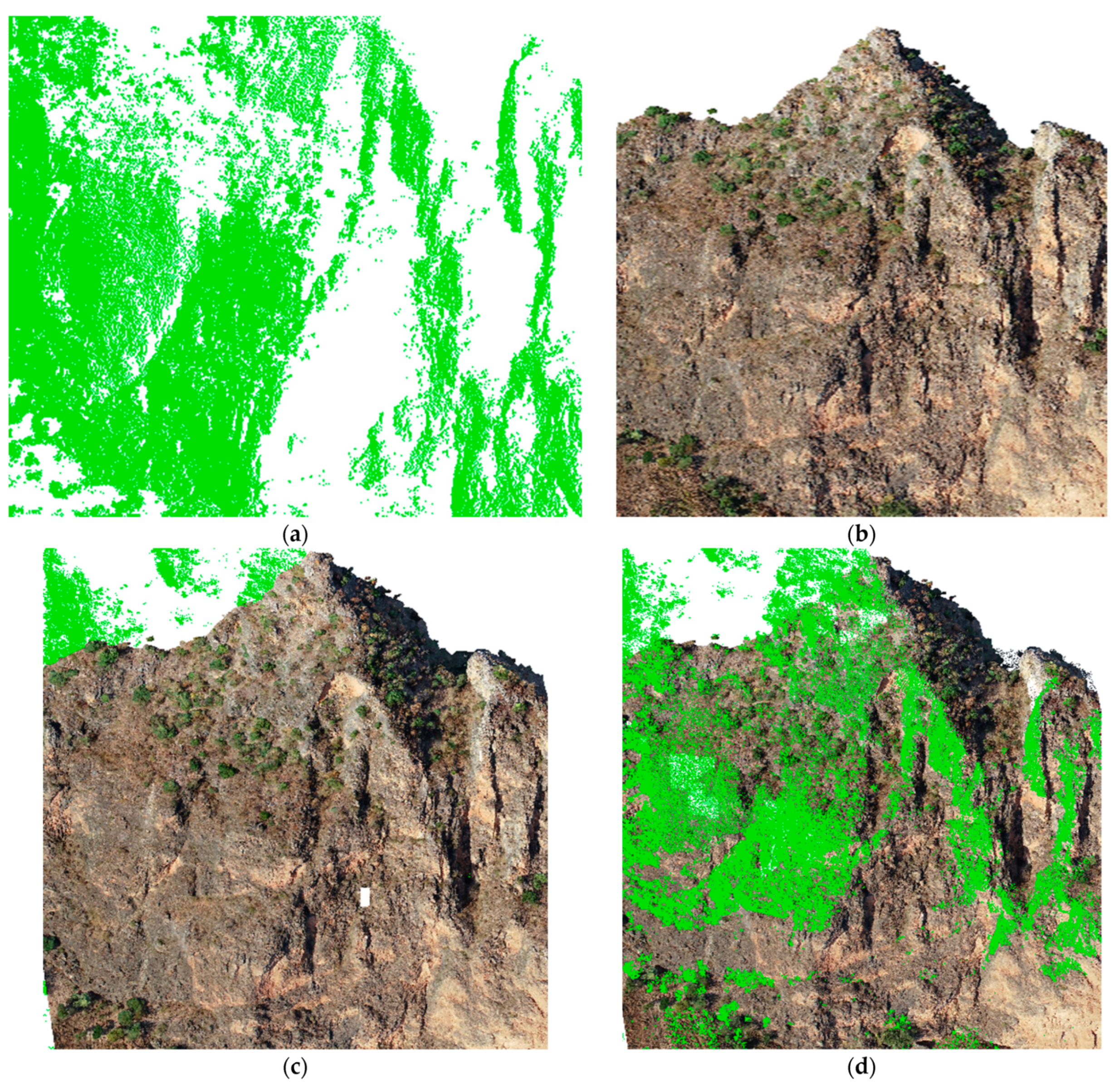
3.3. Multi-Source Point Cloud Fusion

The ground laser point clouds were highly accurate and fast, but some of them had hollow phenomena. UAV photography measurement was wide and easy to use, while photo-distortion easily occurred in depressed areas, resulting in large data errors and low accuracy, difficult to correct by correction algorithms. In addition, high point cloud accuracy is required for the identification of rock discontinuity surfaces. Therefore, the ground 3D laser point cloud was mainly used, together with the use of the UAV photogrammetry point cloud to compensate for the scanned point cloud voids, to achieve the unity of data integrity and high accuracy.

Multi-source point cloud data refer to multiple types of point clouds with different data attributes acquired from multiple sites, multiple time phases, and multiple platforms [17]. Data fusion aims to fuse the data of the same target object according to certain mathematical rules to finally obtain the complete data of the measurement area. In this paper, the ground 3D laser scanning point cloud and UAV tilt photogrammetry point cloud data were processed to achieve multi-point cloud fusion. At present, there are many multi-source point cloud fusion methods, but the common ones are the Iterative closest point (ICP) algorithm [18], the improved ICP algorithm, the unified coordinate system method, etc.

Due to the heterogeneity of multi-source data, it is necessary to standardize the multi-point cloud data and unify the data format as “*.las” before data fusion. The point cloud data from different data sources have their own coordinate systems; thus, it is necessary to transform and unify them under the same coordinate system. Therefore, we fused the point clouds in two steps: first, to roughly fuse the point clouds through a unified coordinate system; second, to precisely fuse them through the improved ICP algorithm.

The unified coordinate system method is based on homonymous points, which can be target spheres or obvious feature points, and it mainly solves the case that the initial positions of data are too far apart. To convert the point cloud data in different coordinate systems to the desired coordinate system, we found more than three sets of homonymous point pairs so that the homonymous point pairs (Pi, Pj) could satisfy the same transformation (R, m, T).

$$\left[\begin{array}{l}X\\ Y\\ Z\end{array}\right]=mR\left[\begin{array}{l}x\\ y\\ z\end{array}\right]+T\left[\begin{array}{l}x0\\ y0\\ z0\end{array}\right]$$

(1)

$$R=\left(\begin{array}{ccc}\cos \alpha & -\sin \alpha & 0\\ \sin \alpha & \cos \alpha & 0\\ 0& 0& 1\end{array}\right)\left(\begin{array}{ccc}\cos \beta & 0& -\sin \beta \\ 0& 1& 0\\ \sin \beta & 0& \cos \beta \end{array}\right)\left(\begin{array}{ccc}1& 0& 0\\ 0& \cos \lambda & -\sin \lambda \\ 0& \sin \lambda & \cos \lambda \end{array}\right)$$

(2)

where m is the scale parameter, R is the rotation matrix, and T is the translation matrix, which denotes the rotation angle along the X, Y, and Z axes. Meanwhile, the coarse alignment accuracy was evaluated by the root-mean-square error (RMSE) based on the selected homonymous point pairs, which is given by

$$RMSE=\sqrt{\frac{{\displaystyle \sum _{i=1}^n{(xi-x\widehat{i})}^2}}{n}}$$

(3)

where n is the number of corresponding point pairs, $xi$ is the Euclidean distance between homonymous pairs after alignment, and $x\widehat{i}$ is the true value of the distance between homonymous pairs.

Based on the five control marker target points laid out, the exact coordinates were obtained in the point cloud (Figure 8) and corresponded to the GPS acquisition CGCS 2000 coordinate points one by one (

Table 2. Point cloud rough registration by unified coordinate system method.

Point	GPS Measured Coordinates			Point Cloud Coordinates			Error
	X/m	Y/m	Z/m	X/m	Y/m	Z/m
B1	551,379.119	2,915,387.696	1729.519	251,963.699	2,916,511.864	1766.708	0.031748
B2	551,383.922	2,915,397.262	1729.033	251,968.764	2,916,521.269	1766.197	0.031388
B3	551,516.047	2,915,430.586	1687.368	252,101.554	2,916,551.698	1724.605	0.045522
B4	551,975.125	2,915,260.500	1654.448	252,557.497	2,916,368.768	1691.321	0.026318
B5	551,980.360	2,915,270.591	1656.444	252,562.979	2,916,378.712	1693.298	0.014648

), and the RMSE = 0.0308554 was calculated according to the fusion effect.

The unified coordinate system method transforms different coordinate systems so that the point clouds collected by both 3D laser scanning and UAV photogrammetry are in CGCS 2000 coordinate system. This completes the rough fusion of multi-source point clouds, but the deviation between different point clouds is large. Therefore, an improved ICP algorithm was used for accurate fusion to complete the multi-source point cloud fusion.

The improved ICP algorithm is based on the original ICP algorithm by adding rotation angle constraints and dynamic iteration coefficients [19]; the algorithm flow is as follows.

(1)

Set the initial value of rigid body transformation $q_0={[R_0,t_0]}^{\mathrm{T}}$, where $R_0$ is the initial rotation matrix and $t_0$ is the initial translation vector;

(2)

Let $P_{s0}=R_0{P}_s+t_0$ and the dynamic iteration coefficient $h=0$;

(3)

Estimate the rotation angle boundary ${\theta }_x\in [{\theta }_{xb}-△{\theta }_x,{\theta }_{xb}+△{\theta }_x],{\theta }_y\in [{\theta }_{yb}-△{\theta }_y,{\theta }_{yb}+△{\theta }_y],{\theta }_z\in [{\theta }_{zb}-△{\theta }_z,{\theta }_{zb}+△{\theta }_z]$, where ${\theta }_{xb},{\theta }_{yb},{\theta }_{zb}$ is the mean value of the rotation angle and $△{\theta }_x,△{\theta }_y,△{\theta }_z$ is the deviation value of the rotation angle;

(4)

Calculate the rotation matrix $R_{k+1}$ and the translation vector matrix $t_{k+1}$, and calculate $q_{k+1}={[R_{k+1},t_{k+1}]}^{\mathrm{T}}$;

(5)

Calculate the amount of change in two adjacent iterations $△q_{k+1}$;

(6)

Calculate $P{s}_{k+1}$ to obtain a new rigid body transformation matrix $(R_{k+1},t_{k+1})$;

$$(R_k,t_k)=\underset{R_k^T{R}_k=I_n,\det (R)=1,t_k}{\arg \min }({\displaystyle \sum _{\min }{‖R_k{P}_s+t_k-P_T‖}_2^2})$$

(4)

(7)

Root-mean-square-error judgment: if $RM{S}_{k+1}-RM{S}_k>\epsilon$, then $h=h+1$; if $\left|RM{S}_{k+1}-RM{S}_k\right|<\epsilon$ or $k>n$, then the algorithm terminates and the iteration ends, where $\epsilon$ is the set threshold and $n$ is the number of iterations.

$$RMS=\sqrt{{\displaystyle \sum _{i=1}^{Ns}{‖R_{k+1}P{s}_{k+1}+t_{k+1}-P_{T_{k+1}}‖}_2^2}}$$

(5)

Through the unified coordinate system and the improved ICP algorithm, the hollow part in the 3D laser point cloud was supplemented by the UAV photogrammetry point cloud, and the fusion of the UAV photogrammetry point cloud and the 3D laser point cloud data was realized. Consequently, we obtained the complete point cloud of the high and steep cliff. At this point, the point cloud data did not have problems such as stratification and deviation, which ensured data integrity while effectively ensuring data accuracy. This laid a foundation for later analysis, as shown in Figure 9.

For the fused point cloud, the error in fusion was counted by intelligent sampling. The smaller the distance between the nearest point pairs, the greater the number of fused point pairs, the lower the number of unfused point pairs, and the better the fusion quality, to test whether its accuracy meets the requirements. See Figure 10 for details. It can be seen that the distance between the nearest point pairs was concentrated below 2.8 m, there were few unregistered point pairs, and the fusion effect of point cloud was better.

4. Intelligent Identification and Information Extraction of Rock Discontinuities

A rock discontinuity is a geometry of faceted extension of a certain thickness in three-dimensional space, so it has certain geometric forms and geometric features, which can be described by spacing, continuity, etc. Based on the multi-source fusion point cloud, the information of the discontinuous surface of the high steep cliff rock was intelligently extracted (Figure 11).

4.1. Point Cloud Normal Vector Calculation

Before conducting point cloud analysis, the normal vector of point cloud needed to be determined based on the spatial distribution of the point cloud first. In the traditional normal vector calculation, for each point xi in the point cloud, a K-Nearest-Neighbor (KNN) algorithm was used to search for the neighborhood points of xi and fit into the surface, and the points in the surface were subjected to principal component analysis (PCA), which was to find eigenvector corresponding to the minimum one. This eigenvector is the normal vector of the fitted surface. However, it was difficult to determine the value of K. Choosing too large or too small a value for K could cause either over-segmentation or under-segmentation of the point cloud, resulting in a large error in the calculation of the normal vector of the point cloud. Therefore, the normal vector calculation of the rock mass point cloud was based on the improved KNN search algorithm.

Affected by point cloud acquisition equipment, methods, and spatial differences of features, the number of point clouds of different target objects in the same neighborhood range varies greatly. At this time, if a single-scale neighborhood is used, it will affect the accurate expression of local geometric features and cause the uncertainty of neighborhood features to increase, thus causing a large error in the calculation of normal vector. According to the entropy principle, for any point in the point cloud, the amount of information contained in its neighborhood range can be expressed by the information entropy, and the smaller the entropy value is, the less information is contained in the neighborhood of the point, and the higher the certainty of the point in any dimensional range, which can best express the actual distribution characteristics of the object surface [20], and the normal vector estimation is more reasonable. Therefore, using the neighborhood range information entropy, the best neighborhood radius K value can be obtained through the entropy function minimization constraint criterion, that is:

$$E_f=-{\displaystyle \sum _i{p}_i\log p_i}=-p_1\ln p_1-p_2\ln p_2-p_3\ln p_3$$

(6)

$$(p_1,p_2,p_3)=\left[\frac{\sqrt{{\lambda }_1}-\sqrt{{\lambda }_2}}{\sqrt{{\lambda }_1}},\frac{\sqrt{{\lambda }_2}-\sqrt{{\lambda }_3}}{\sqrt{{\lambda }_1}},\frac{\sqrt{{\lambda }_3}}{\sqrt{{\lambda }_1}}\right]$$

(7)

$$R_{best}=\underset{r\subset \left[R_{\min },R_{\max }\right]}{{\displaystyle \arg \min (E_f)}}$$

(8)

where $p_1+p_2+p_3=1$, ${\lambda }_1,{\lambda }_2,{\lambda }_3$ are the eigenvalues of the covariance matrix of the neighborhood point set; $R_{best}$ is the optimal neighborhood radius; $E_f$ is the information entropy of the neighborhood range; $\left[R_{\min },R_{\max }\right]$ is the neighborhood radius search interval, which is suggested to be $\left[0.02\mathrm{m},0.5\mathrm{m}\right]$ [20].

After completing the K-nearest-neighbor search, linear fitting based on least squares fitting is performed to obtain the plane equation.

$$Ax+By+C=Z,\left[\begin{array}{ccc}x& y& 1\end{array}\right]\left[\begin{array}{c}A\\ B\\ C\end{array}\right]=\left[Z\right]$$

(9)

Let the coordinates of the k + 1 points on the discontinuity of the rock mass be $\left(x_1,y_1,z_1\right),\left(x_2,y_2,z_2\right)\cdots \left(x_{k+1},y_{k+1},z_{k+1}\right)$, then

$$\begin{array}{l}\left[\begin{array}{ccc}{x}_1& y_1& 1\\ ⋮& ⋮& ⋮\\ x_{k+1}& y_{k+1}& 1\end{array}\right]\left[\begin{array}{c}A\\ B\\ C\end{array}\right]=\left[\begin{array}{c}{Z}_1\\ ⋮\\ Z_{k+1}\end{array}\right]\\ \\ Let\left[\begin{array}{ccc}{x}_1& y_1& 1\\ ⋮& ⋮& ⋮\\ x_{k+1}& y_{k+1}& 1\end{array}\right]=X,\left[\begin{array}{c}A\\ B\\ C\end{array}\right]=A,\left[\begin{array}{c}{Z}_1\\ ⋮\\ Z_{k+1}\end{array}\right]=Z\end{array}$$

(10)

Then, find A so that $\phi \left(\mathrm{A}\right)=|AX-Z|$ obtains the minimum value, that is, the plane equation and its normal vector are obtained by local surface fitting. Let the normal vector of the discontinuous surface of the rock mass be $n\left(A,B,C\right)$; then, the rock mass orientation information (dip angle, dip direction) can be calculated by the following equation [21].

The angle between the strike line of the rock discontinuity and the due north is

$$\beta =\frac{180\arctan \left|\frac{B}{A}\right|}{\pi }$$

(11)

The dip angle is

$$\alpha =\frac{180\arctan \left(\frac{\sqrt{A^2+B^2}}{\left|C\right|}\right)}{\pi }$$

(12)

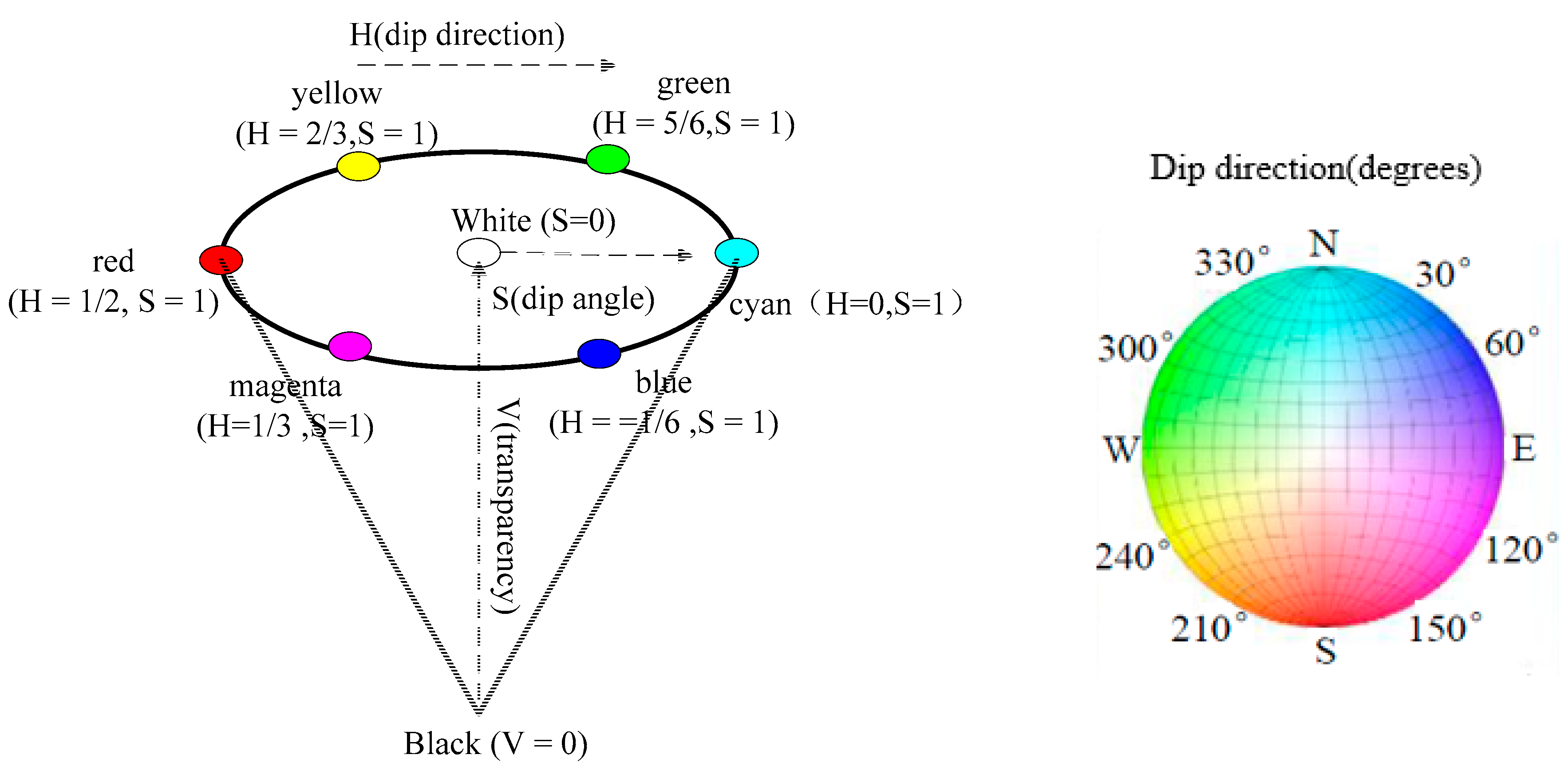
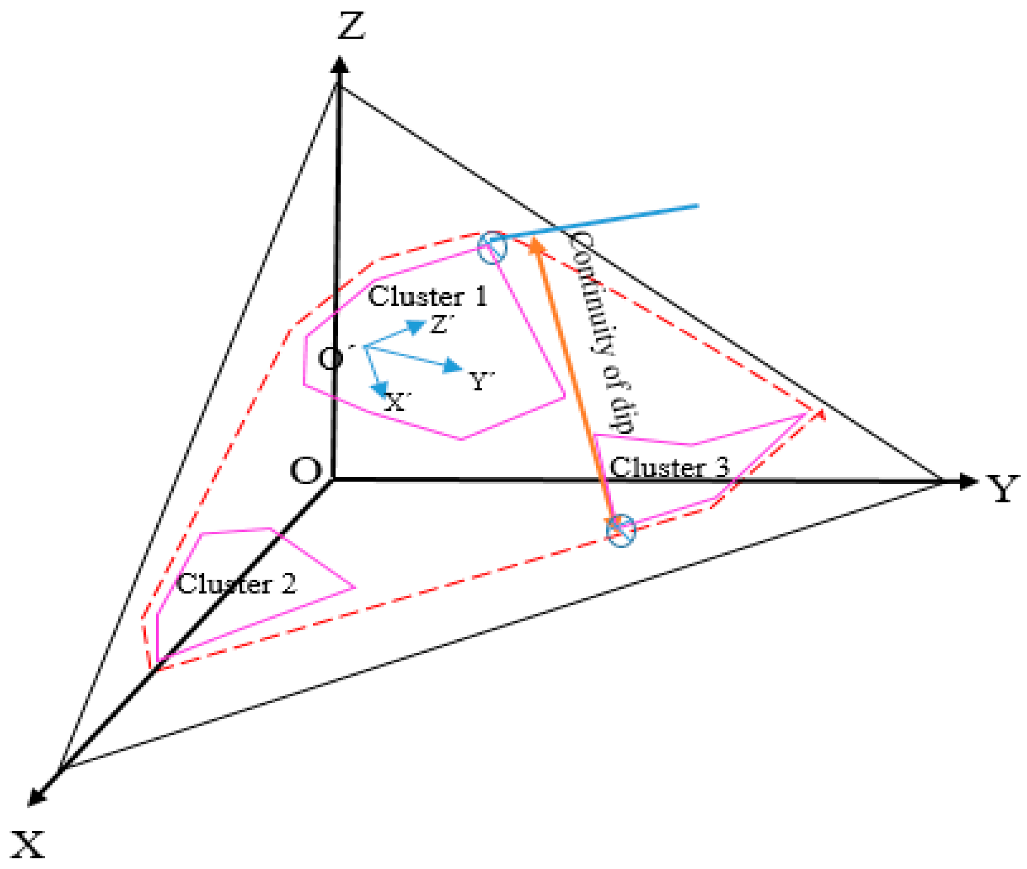
4.2. HSV 3D Reconstruction and Clustering Analysis

Using point cloud normal vectors, combined with Equations (11) and (12), the rock yield can be calculated quickly, but due to the significant number of steep cliff point clouds, hundreds or thousands of sets of yields can be obtained by this method, and all yields show the same color, which cannot visualize the spatial distribution of structural surfaces. Therefore, we implemented the hexagonal pyramid model (hue saturation lightness value, HSV) spatial coloring of point clouds based on Matlab, which assigns a specific color to each discontinuous in space. HSV is a combination of the Schmidt projection network and HSV color, and its color space is a cone. Using the circumference of the base of the cone represents the hue (H) and takes values from 0 to 360°. Cyan is 0°, blue is 60°, magenta is 120°, red is 180°, yellow is 240°, and green is 300°. S is saturation, where the greater the proportion of the spectrum, the closer the color is to the spectral color, and the greater its saturation; luminosity (V) indicates the shade of the color (Figure 12). In our study, H corresponds to the dip direction, S corresponds to the dip angle, and V is the transparency set to the maximum value of 1. Among them, there are 361 colors in the color phase H corresponding to direction, and the distribution of rock production (dip angle and dip direction) can be effectively identified by observing the changes of different colors.

In order to accurately obtain the information about the discontinuous surface of the rock mass, a clustering analysis of the point cloud is required before information extraction. Therefore, in this paper, a combination of kernel density estimation (KDE) and the density-based spatial clustering of applications with noise (DBSCAN) algorithm was used to complete the rock discontinuity clustering. First, the KDE algorithm was used to identify the peaks representing the direction of the 3D point cloud and its adjacent point clouds, and then the DBSCAN algorithm was used to perform the clustering operation for further clustering analysis. In addition, we adopted the research results of Riquelme et al. [22,23]. The two parameters of DBSCAN were set as Minpts = 4, and Eps was the average distance between each point and the surrounding 4 neighboring points plus 2 standard deviations.

4.3. Rock Discontinuity Surface Parameter Extraction

(1)

Spacing

The rock discontinuity spacing is an important indicator to measure rock development and is used to reflect the integrity of rock masses [24]. The International Society of Rock Mechanics (ISRM) defines the discontinuity spacing as the vertical distance between two fissures on the outcrop. Therefore, the discontinuity set extractor (DSE) based on Matlab [22] was used to extract the spacing information for each set of rock discontinuities after clustering. The spacing measured in DSE takes into account two cases of rock discontinuities in the same set, fully continuous and not fully continuous, and is calculated by measuring the orthogonal distance between a given cluster and the nearest-neighbor cluster.

$$D_{ij}=-\frac{A_{ij}}{n}{\displaystyle \sum _{k=1}^n{x}_{ij}^k}--\frac{B_{ij}}{n}{\displaystyle \sum _{k=1}^n{y}_{ij}^k}--\frac{C_{ij}}{n}{\displaystyle \sum _{k=1}^n{z}_{ij}^k}$$

(13)

where $(x_{ij}^k,y_{ij}^k,z_{ij}^k)$ are the coordinates of the k point in a cluster, and $A_{ij},B_{ij},C_{ij}$ are its normal vectors.

(2)

Continuity

ISRM states that the continuity of a rock mass is the extent or size of the area along the planar discontinuity, and in two dimensions, the trace length is often used to characterize the continuity of a rock plane [25]. Thus, we calculated the continuity of the structural plane by the Matlab-based DSE program. It can measure the true continuity by calculating the trace length of each cluster’s strike and dip [1]. For the clusters after clustering, a coordinate system is established with the dip direction as the x-axis and the strike direction as the y-axis, and each cluster of the original coordinate system (the origin of the coordinate system is the center of mass) is transformed with the following transformation matrix.

$$R=\left[\begin{array}{ccc}\cos \beta \sin \alpha & -\cos \alpha & \sin \beta \sin \alpha \\ \cos \beta \cos \alpha & \sin \alpha & \sin \beta \cos \alpha \\ -\sin \beta & 0& \cos \beta \end{array}\right]$$

(14)

where $\alpha ,\beta$ are the dip direction and dip angle of the discontinuous sets, respectively, $O-XYZ$ is the original coordinate system, and $O^{\prime }-X^{\prime }{Y}^{\prime }{Z}^{\prime }$ is the transformed coordinate system. The ductility is extracted in the directions of dip $O^{\prime }{X}^{\prime }$ and strike $O^{\prime }{Y}^{\prime }$. $O^{\prime }{Z}^{\prime }$ is orthogonal to the plane $O^{\prime }{X}^{\prime }{Y}^{\prime }$, and its normal vector is that after the plane is clustered (Figure 13). Let the number of the discontinuous set be $i$ and the number of the cluster be $j$; the point set $x_{(i,j)}$ can be obtained. If ${x^{\prime }}_{(i,j)}$ is the local coordinate of $x_{(i,j)}$, the equation of the extension length in the inclination direction is

$$L=\max ({x^{\prime }}_{(i,j)})-\min ({x^{\prime }}_{(i,j)})$$

(15)

4.4. Accuracy Check

In past studies, Chen [15] compared the clustering results with the Riquelme method, and Zhang [13], Zhao [26], Xu [27], Gao [28], and Guo [29] compared the clustering results with field measurement data or polar isodensity maps to verify the accuracy of the results. Therefore, we took the local point cloud on the left side of the steep cliff as an example, and used three ways to verify the applicability of the proposed method in the high steep cliff area.

The first is to compare the clustering results with the actual occurrence of the field geological compass. Figure 14 shows the results of local rock clustering on the left side of the steep cliff using our method, showing that there were three groups of joint faces in this part, J1 cyan (134∠80), J2 yellow (177∠80), and J3 dark red (209∠73). Meanwhile, the measured data, collected in the field survey by the staff of the Second Yunnan Geological Engineering Survey Institute, were 134∠82, 177∠80, and 213∠74, respectively. The average inclination error of group J1 was about 2°, that of group J2 was about 0°, and that of group J3 was about 4°. The average error of dip angle was 2° and the average error of dip direction was 1°, which satisfied the requirement of ±5° for the angle measurement error in the geological rock discontinuity survey [30].

Secondly, Dips 7.0 was used to draw the measured poles isodensity map, which was compared with the poles isodensity map obtained by extracting the rock discontinuity by the method in this paper. The results were similar and met the analysis requirements, as shown in Figure 15.

Thirdly, the clustering results were compared with Riquelme method [22], and the results were similar (

Table 3. Comparison of clustering results between the proposed method and Riquelme’s method.

Discontinuity Set	Clustering Results		Riquelme Method		Error
	Dip (°)	Direction (°)	Dip (°)	Direction (°)	Dip (°)	Direction (°)
1	80	134	81.213	133.857	1.213	−0.143
2	80	177	80.015	177.354	0.015	0.354
3	73	209	70.330	209.214	0.330	0.214

).

5. Results and Analysis

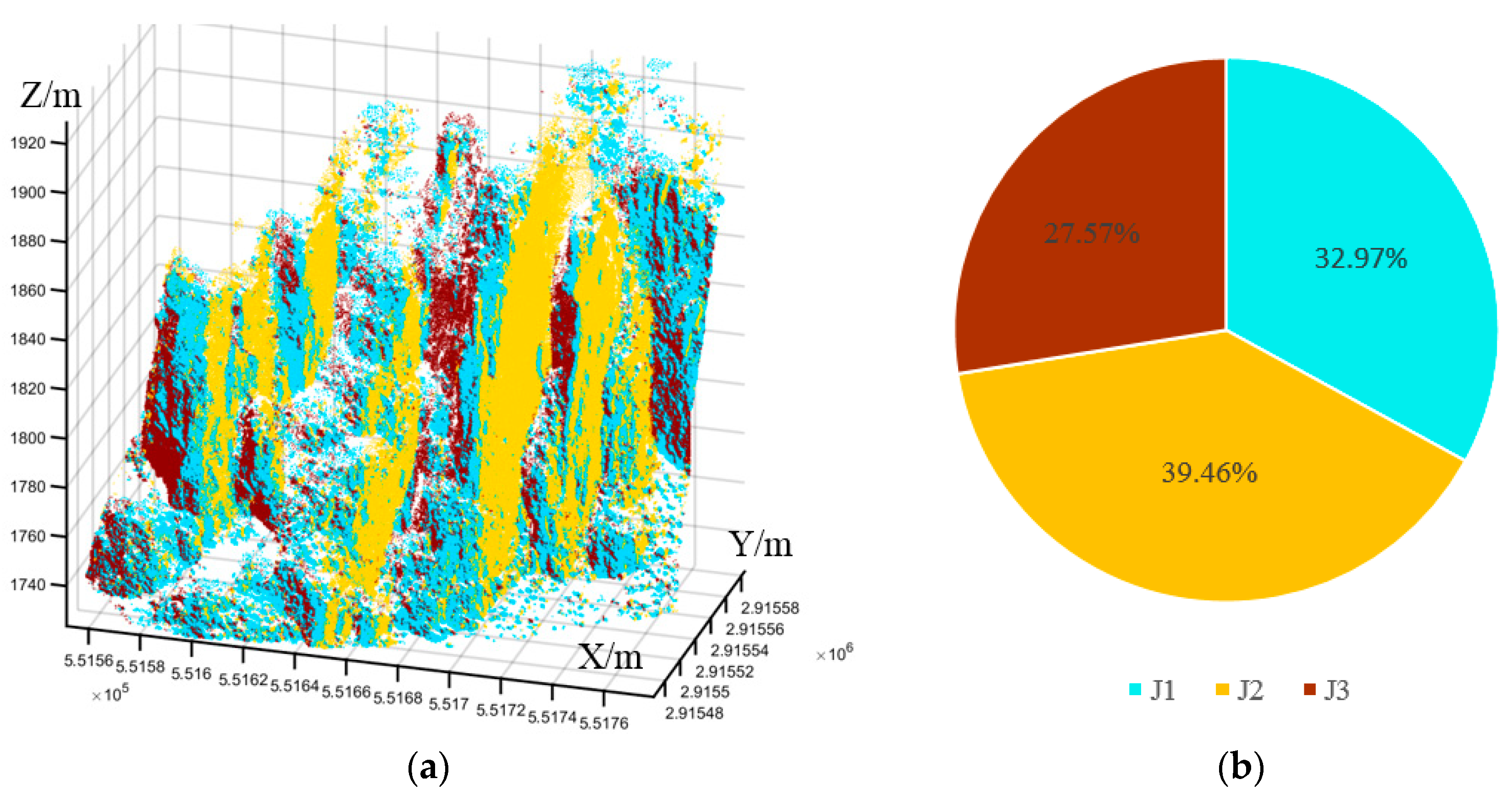
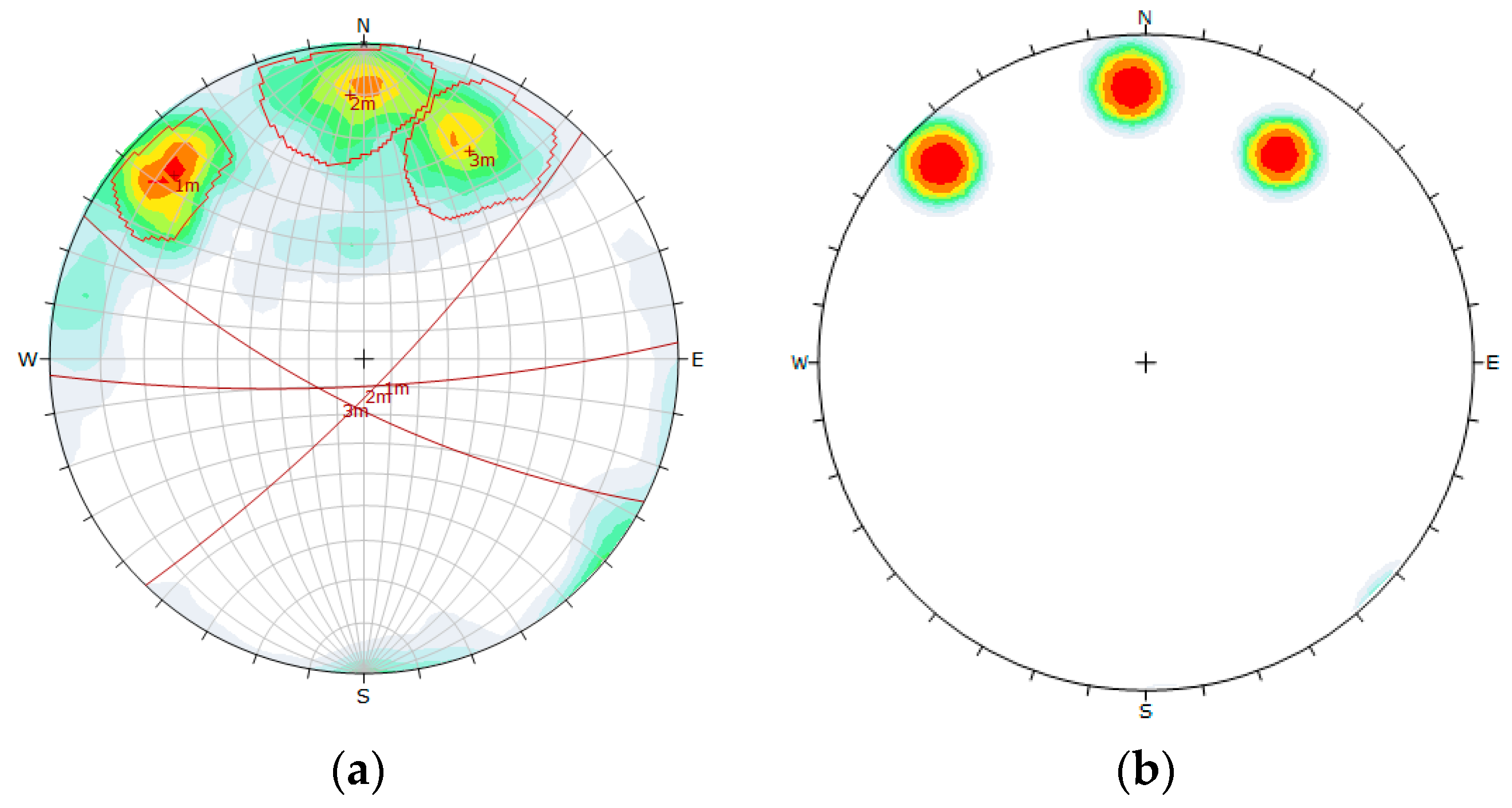
5.1. Grouping of Rock Discontinuity Surfaces

We selected about 840,000 rock wall point clouds. Figure 16a,b show that the rock tendency was mainly concentrated in 120°–240°, with a few parts located at 60°, and the overall steep cliff slope was relatively steep. In addition, the extracted rock discontinuities were clustered and six groups of structural faces (J1–J6) were identified, among which J6 was the level and the yield was 184∠88.9, and J4 and J5 were steeply inclined discontinuities with a large dip angle. The occurrences for J1–J5 were 204∠81, 176∠39.4, 211∠45.2, 129∠86.9, and 138∠88.6, respectively. The calculation of the distribution of discontinuous surfaces showed that the discontinuous surface sets J1, J4, and J5 were larger, with J1 (26.92%) as the largest and J6 (6.49%) as the smallest, as shown in Figure 16.

5.2. Rock Discontinuity Face Spacing

The results of calculating the spacing of rock discontinuities are shown in Figure 17. Its ordinate indicates the probability density function, and the abscissa indicates the spacing. The overall obeyed a negative exponential distribution. In the case of noncomplete continuity, the rock discontinuity surface J4 was 32.3786 m and had the largest spacing, while J1 was only 9.09 m and had the smallest spacing, which are shown in

Table 4. Summary of the distance between discontinuous planes in each group of cliff walls.

	J1	J2	J3	J4	J5	J6
Discontinuous face spacing of continuous lower rock mass	9.09	19.0	14.96	32.38	9.38	11.70
Discontinuous face spacing of discontinuous lower rock mass	4.46	6.58	6.91	31.33	2.47	7.14

.

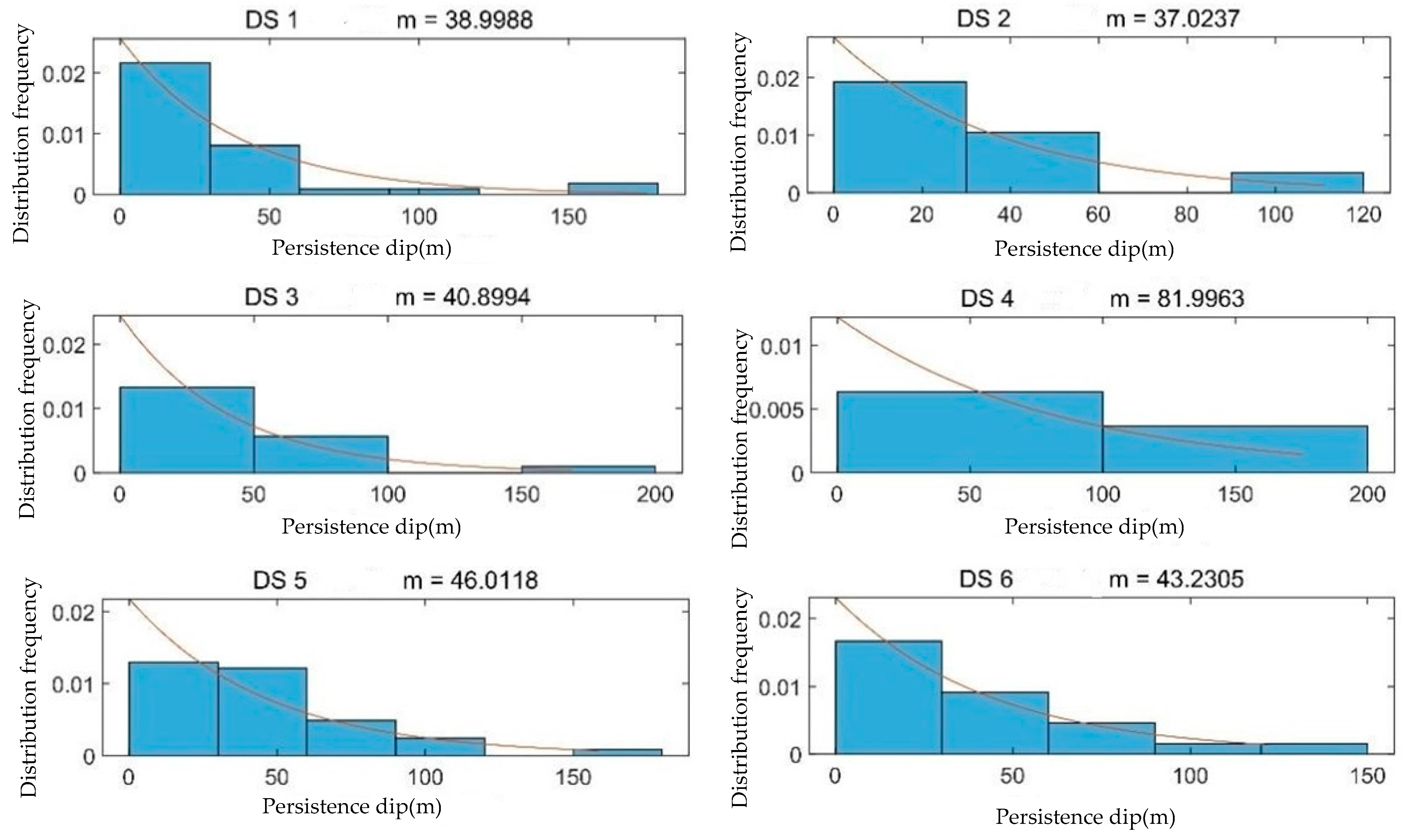
5.3. Continuity of Rock Discontinuity Surface

Figure 18 shows the histogram of continuity of the rock mass structure plane, whose ordinate indicates the distribution frequency and abscissa indicates the continuity length, which are the standard normal distribution. It can be seen that the continuity of the rock mass was very good, and its extension length was >30 m. The continuity of the rock mass plane J4 reached 81.99, with the largest extension length, and the continuities of J3, J5, and J6 were all equal, around 40 m.

6. Discussion

Using ground 3D laser scanning and UAV photogrammetry technology, we identified the rock discontinuity and extracted information of the high and steep cliff on the south side of Laojun Peak, which has the following characteristics:

(1)

Multi-source point cloud fusion technology ensures the accuracy and efficiency of rock mass point cloud data acquisition. In past studies, almost all scholars used a single method to obtain three-dimensional point cloud data of rock masses and extract rock discontinuities. For example, Ye [3], Ge [11], and Ning [31] all adopted ground 3D laser scanning technology or UAV photogrammetry technology to obtain 3D point cloud data of rock masses in the study area. However, in most cases, a single way of measuring easily leads to obtaining point cloud data that are incomplete or have poor precision. For example, Liang [10] once pointed out that the accuracy of ground three-dimensional laser scanning technology is higher, but it is greatly influenced by the rock mass discontinuity surface inclination. This is followed by the small-angle laser launch of the rock mass discontinuity, whose data quality is poorer. Point cloud data holes easily appear, and a variety of ways should be used for supplementary testing. Therefore, our proposed multi-source point cloud fusion technology ensures the integrity and accuracy of rock mass point cloud data. However, there are drawbacks to this approach. If the cavity region of the 3D laser scanning point cloud and the distorted region of UAV photogrammetry data are in the same position, the multi-source point cloud fusion method will lose its function. Therefore, in the early stage of measurement, it is necessary to carry out a field survey and make a complete measurement plan.

(2)

Based on the 3D point cloud, the normal vector of the point cloud is calculated using an improved nearest-neighbor search algorithm and transformed into the rock body yield (dip angle and dip direction). Combined with KDE and DBSCAN clustering algorithms, the rock body discontinuities are grouped dominantly and the yield spacing and continuity of the rock body are calculated. This method can quickly obtain the rock mass production information, and the results are similar to the measured production and meet the accuracy requirements. In addition, this method can greatly reduce the geologists’ field workload and lower the time cost. However, this method also has some drawbacks, as Chen et al. [15] pointed out; when discontinuous surfaces are extracted from 3D point clouds and clustered using the DBSCAN algorithm, although the method has good robustness to noisy points, it still needs to combine density peaks and manually set the number of clusters, and the degree of automation and intelligence needs to be improved.

7. Conclusions

Based on the collection and fusion of multi-source data, this paper performed intelligent identification and information extraction of the rock surface discontinuity for the high and steep cliffs on the south side of Laojun Peak in Huidong County. The study achieved good results and solved the problem of the manual inability to obtain the rock mass orientation information under special circumstances, and provided an effective reference for engineering geological investigation. Based on the extracted geometric information of rock discontinuities, a kinematic analysis model can be constructed, which can provide basic data for rock stability evaluation. The main conclusions are as follows.

(1)

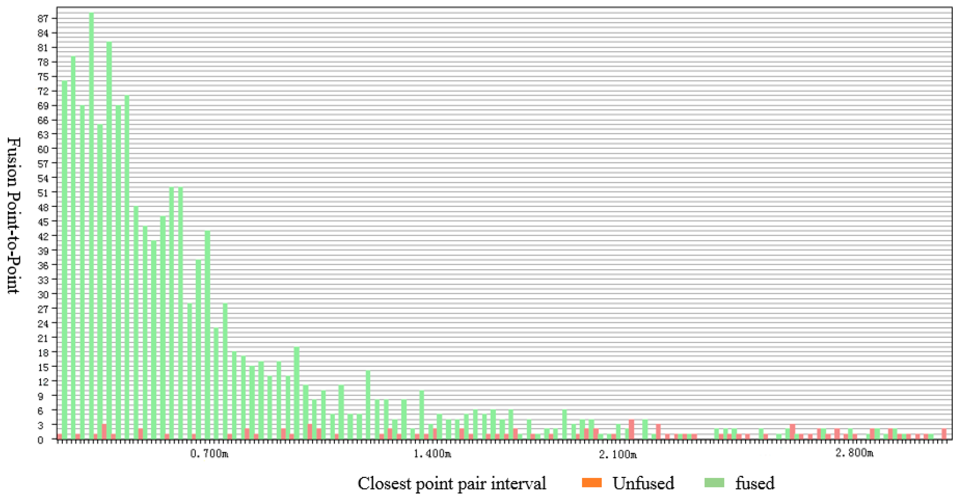
Ground 3D laser scanning and UAV photogrammetry technology can rapidly and efficiently obtain high-density, high-precision 3D point cloud information under complex geological environment conditions. However, both technologies have their drawbacks. The ground 3D laser scanning technology can achieve highly precise measurement with a scanning error of 2 mm–6 mm, but it is difficult to obtain complete point clouds under complex terrain environments such as those with large height differences. The UAV tilt photogrammetry technology is prone to camera distortion and blurred images, which leads to low measurement accuracy and large data errors. By adopting the unified coordinate system and improved ICP algorithm for point cloud fusion, the photogrammetric point cloud is used to supplement the missing part of the 3D laser point cloud, which not only ensures data integrity but also data accuracy. The fusion accuracy error is less than 2.8 m with a better fusion effect. This method can provide an accurate data source for the intelligent identification of discontinuous surfaces of special geological rock masses, such as high and steep cliffs, and ensures the accuracy of the identification. This is of great importance in geological investigations.

(2)

The spatial index is established by the Kd-tree algorithm, and the optimal scale of the adaptive neighborhood is obtained by neighborhood information entropy, which overcomes the problem of over-segmentation or under-segmentation of point clouds brought by too large or too small a neighborhood radius K, and ensures the accuracy of the point cloud normal vector and rock mass orientation calculation.

(3)

Based on the multi-source fusion of point clouds, we use an improved KNN search algorithm, a KDE algorithm combined with the DBSCAN algorithm, to intelligently extract rock discontinuity surface information, which provides a complete technical process and method to obtain highly precise rock mass orientation information under complex geological conditions. It helps to further analyze rock stability.

References

- Ning, H. Identification and Information Extraction of Rock Discontinuity Surface Based on 3D Laser Scanning. Master’s Thesis, Chengdu University of Technology, Chengdu, China, 2020. [Google Scholar]
- Jia, S.G.; Jin, A.B.; Zhao, Y.Q. Application of UAV photogrammetry in geological investigation of high and steep slopes. Geotechnics 2018, 39, 1130–1136. [Google Scholar]
- Ye, Z.; Xu, Q.; Liu, Q.; Dong, X.J.; Wang, X.C.; Ning, H. Application of Unmanned Aerial Vehicle Oblique Photogrammetry to Investigation of High Slope Rock Structure. Geomat. Inf. Sci. Wuhan Univ. 2020, 45, 1739–1746. [Google Scholar]
- Xu, D.; Feng, X.T.; Li, S.J.; Wu, S.Y.; Qiu, S.L.; Zhou, Y.Y.; Gao, Y.H. Research on key information extraction technology of deformation and damage characteristics of rock masses in Jinping underground laboratory based on 3D laser scanning. Geotech. Mech. 2017, 38, 488–495. [Google Scholar]
- Feng, M. Research on 3D Modeling and Rock Joint Information Extraction of High Steep Cliffs. Master’s Thesis, Kunming University of Science and Technology, Kunming, China, 2020. [Google Scholar]
- Jing, H.D.; Li, Y.H.; Zhang, Z.H.; Liu, Z.S. Information extraction of rock discontinuity surface based on 3D laser scanning. J. Northeast. Univ. 2015, 36, 280–283. [Google Scholar]
- Li, S.J.; Feng, X.T.; Wang, C.Y.; Hudson, J.A. ISRM suggested method for rock fractures observations using a borehole digital optical televiewer. Rock Mech. 2013, 46, 635–644. [Google Scholar] [CrossRef]
- Wu, X. Geometric Information Extraction of Rock Mass Structural Plane Based on 3D Laser Point Cloud. Master’s Thesis, Jilin University, Changchun, China, 2022. [Google Scholar]
- Ge, Y.F.; Tang, H.M.; Xia, D.; Wang, L.Q.; Zhao, B.B.; Teaway, J.W.; Chen, H.Z.; Zhou, T. Automated measurements of discontinuity geometric properties from a 3D-point cloud based on a modified region growing algorithm. Eng. Geol. 2018, 242, 44–54. [Google Scholar] [CrossRef]
- Liang, Y.F.; Pei, X.J.; Cui, S.H.; Huang, R.Q.; Li, T.T.; Xu, X.N.; Dong, X.J.; Tan, L.Y.; Yang, H.Y. Structural characteristics analysis of landslide damage boundary rock based on ground 3D laser point cloud. J. Rock Mech. Eng. 2021, 40, 1209–1225. [Google Scholar]
- Ge, Y.F.; Xia, D.; Tang, H.M.; Zhao, B.B.; Wang, L.Q.; Chen, Y. Intelligent identification and extraction of geometric properties of rock discontinuities based on terrestrial laser scanning. Chin. J. Rock Mech. Eng. 2017, 36, 3050–3061. [Google Scholar]
- Chen, N.; Cai, X.M.; Xia, J.W.; Zhang, S.H.; Jiang, Q.H.; Shi, C. Intelligent interpretation of rock discontinuity surfaces based on 3D laser point cloud technology. Geoscience 2021, 46, 2351–2361. [Google Scholar]
- Zhang, P.; Du, K.; Tannant, D.D.; Zhu, H.H.; Zheng, W.B. Automated method for extracting and analysing the rock discontinuities from point clouds based on digital surface model of rock mass. Eng. Geol. 2018, 239, 109–118. [Google Scholar] [CrossRef]
- Wang, P.T.; Tan, T.; Huang, Z.J.; Ren, F.H.; Cai, M.F. Research on rapid identification method of rock discontinuity information based on 3D point cloud. J. Rock Mech. Eng. 2021, 40, 503–519. [Google Scholar]
- Chen, J.Q.; Zhu, H.H.; Li, X.J. Automatic extraction of discontinuity orientation from rock mass surface 3D point cloud. Comput. Geosci. 2016, 95, 18–31. [Google Scholar] [CrossRef]
- Li, Z.B.; Xia, Y.H.; Bai, H.Q. MAPTEK I-Site 8200ER 3D laser scanner goniometric accuracy study. J. Zhejiang Agric. Sci. 2017, 58, 1462–1464. [Google Scholar]
- Yang, B.S.; Liang, F.S.; Huang, R.G. Research progress, challenges and trends in 3D laser scanning point cloud data processing. J. Surv. Mapp. 2017, 46, 1509–1516. [Google Scholar]
- Besl, P.J.; McKay, N.D. Method for Registration of 3-D Shapes. In Proceedings of the Sensor Fusion IV: Control Paradigms and Data Structures, Boston, MA, USA, 12–15 November 1991; pp. 586–606. [Google Scholar]
- Zhao, F.Q. Point Cloud Distribution Algorithm Based on Improving ICP. In Research on the Optimal Alignment Method of Point Cloud Model; Harbin Institute of Technology Press: Harbin, China, 2018; pp. 75–76. [Google Scholar]
- Ma, W.F.; Wang, C.; Wang, J.L.; Zhou, J.C.; Ma, Y.Y. A residual clustering method for fine extraction of laser point cloud transmission lines. J. Surv. Mapp. 2020, 49, 883–892. [Google Scholar]
- Dong, X.J. Comprehensive Application Research of 3D Spatial Imaging Technology in Geological Engineering. Ph.D. Thesis, Chengdu University of Technology, Chengdu, China, 2015. [Google Scholar]
- Riquelme, A.J.; Abellán, A.; Tomás, R.; Jaboyedoff, M. A new approach for semi-automatic rock mass joints recognition from 3D point clouds. Comput. Geosci. 2014, 68, 38–52. [Google Scholar] [CrossRef] [Green Version]
- Riquelme, A.; Tomás, R.; Cano, M.; Pastor, J.L.; Abellán, A. Automatic mapping of discontinuity persistence on rock masses using 3D point clouds. Rock Mech. Rock Eng. 2018, 51, 3005–3028. [Google Scholar] [CrossRef]
- Zhao, W.; Tang, C.A. Measurement theory of rock discontinuity face spacing and trace length. China Min. 1998, 3, 36–38. [Google Scholar]
- Fan, L.M.; Huang, R.Q. A new method for estimating the trace length of rock discontinuities and its engineering application. J. Rock Mech. Eng. 2004, 1, 53–57. [Google Scholar]
- Zhao, J.B.; Zhang, Y.S.; Li, X.S. Automatic identification method of rock mass structural plane based on photogrammetric 3D point cloud. Sci. Technol. Eng. 2017, 17, 240–244. [Google Scholar]
- Xu, W.T.; Zhang, Y.S.; Li, X.Z.; Wang, X.Y.; Ma, F.; Zhao, J.B.; Zhang, Y. Extraction and statistics of discontinuity orientation and trace length from typical fractured rock mass: A case study of the Xinchang underground research laboratory site, China. Eng. Geol. 2020, 269, 105553. [Google Scholar] [CrossRef]
- Gao, F.; Chen, D.P.; Zhou, K.P.; Niu, W.J.; Liu, H.W. A fast clustering method for identifying rock discontinuity sets. KSCE J. Civ. Eng. 2019, 23, 556–566. [Google Scholar] [CrossRef]
- Guo, J.T.; Liu, S.J.; Zhang, P.N.; Wu, L.X.; Zhou, W.H.; Yu, Y.N. Towards semi-automatic rock mass discontinuity orientation and set analysis from 3D point clouds. Comput. Geosci. 2017, 103, 164–172. [Google Scholar] [CrossRef]
- Li, S.Q.; Zhang, H.C.; Liu, R.Y. UAV photogrammetry for semi-automatic statistics of rock discontinuity surface production. Sci. Technol. Eng. 2017, 17, 18–22. [Google Scholar]
- Ning, H.; Dong, X.J.; Liu, Q.; Ye, Z.; Guo, C.; Liang, Y.F. Using point cloud normal vector to realize rock mass structural plane recognition. Geomat. Inf. Sci. Wuhan Univ. 2022, 1–13. [Google Scholar]