Abstract
This paper provides an overview of the different deep convolutional neural network (DCNNs) architectures that have been investigated in the past years for the generation of synthetic computed tomography (CT) or pseudo-CT from magnetic resonance (MR). The U-net, the Atrous-net and the Residual-net architectures were analyzed, implemented and compared. Each network was implemented using 2D filters and 3D filters with 2D slices and 3D patches respectively as inputs. Two datasets were used for training and evaluation. The first one is composed by pairs of 3D T1-weighted MR and Low-dose CT images from the head of 19 healthy women. The second database contains dual echo Dixon-VIBE MR images and CT images from the pelvis of 13 colorectal and 6 prostate cancer patients. Bone structures in the target anatomy were key in choosing the right deep learning approach. This work provides a deep explanation of the architectures in order to know which DCNN fits better each medical application. According to this study, the 3D U-net architecture would be the best option to generate head pseudo-CTs while the 2D Residual-net provides the most accurate results for the pelvis anatomy.
1. Introduction
Computed tomography (CT) provides the photon attenuation information that is required in positron emission tomography (PET). Therefore, CT has been used for PET attenuation correction (AC) and for external beam radiation therapy (EBRT) planning since the appearance of the first PET/CT in 1997 [1]. In recent years, the number of combined PET/MR scanners has increased among medical centres [2]. Thus, the interest in replacing the CT scanners with magnetic resonance (MR) imaging has raised since MR provides greater tissue contrast as well as other complementary information such as perfusion or diffusion. Additionally, MR decreases the use of ionizing radiation, specially in the AC for PET imaging. MR Early developments made use of fat and water separation or other specific MR sequences (i.e., UTE, ZTE) to estimate AC maps [3,4]. However, the AC maps estimated using MR imaging have wide discrepancies with the AC maps calculated using the CT [5,6]. The last decade has seen a renewed interest in MR-only workflows for PET imaging and radiotherapy. This way, several works have proposed the synthesis of CT volumes from MR images (pseudo-CT) using computer vision techniques. The first approaches used traditional image processing and machine learning strategies, such as segmentation-based methods [7,8,9,10,11], atlas-based methods [12,13,14,15,16,17] or learning-based methods [18,19,20]. These approaches present several disadvantages, such as the need of an accurate spatial normalization to a template space, the assumption of mostly normal anatomy, or the problem of accommodating a large amount of training data. These problems have been solved in the last few years with the advent of new techniques based on Deep Convolutional Neural Networks (DCNN). The use of DCNNs has also improved the quality of the results while reducing the time for pseudo-CT synthesis.
According to our knowledge, the first approach that adopted deep learning to generate a pseudo-CT from an MR scan was presented by [21]. This work proposed a DCNN that used a U-net architecture [22] performing 2D convolutions. The network received axial slices from a T1-weighted volume of the head as input, and tried to generate the corresponding slices from a registered CT scan. Their architecture incorporated unpooling layers in the up-sampling steps of the U-net and Mean Absolute Error (MAE) as loss function. Their results were compared to an atlas based method [23], obtaining favorable results in accuracy and computational time (close to real-time). In contrast, the work of [24] explored a similar architecture to segment air, bone, and soft tissue instead of generating the continuous pseudo-CT. They used a set of 3D T1-weighted head volumes as well. In this case, they incorporated a nearest-neighborhood interpolation in the up-sampling steps of the U-net. Additionally, as they were classifying instead of regressing, they employed a multi-class cross-entropy loss metric, which is usually easier to optimize than the L1 or L2 error. The deep learning approach performed better than a Dixon-based approach and took less than 0.5 min to generate the pseudo-CT segmentation. Several works made use of more sophisticated network architectures and training pipelines. The work by [25] proposed a 3D neural network with dilated convolutions to avoid the use of pooling operations. They also explored the advantages of residual connections [26] and auto-context refinement [27]. For training, they employed an adversarial network that tried to differentiate between real CTs and pseudo-CTs [28]. They used 3D patches from T1 volumes from head and pelvis as input, and compared their results against traditional methods such as atlas registration, sparse representation and Random Forest with auto-context. Their method outperformed all of these traditional methods. A similar approach was proposed by [29], who trained a 2D DCNN that incorporated the residual blocks from Resnet [26] and an adversarial strategy [28] for training. More recent works used MR Dixon images as input to the network, which are the images typically acquired for AC in commercial PET-MR scanners. Dixon sequences include 4 images: water, fat, in phase and out-of-phase. In addition, the work by [30] provides better bone depiction than Dixon images by adding a Zero-echo time MRI volume. They used a 3D U-net architecture with transposed convolutions as up-sampling layer. In contrast, the work by [31] proposed a 2D U-net architecture with transposed convolutions as up-sampling layer using only Dixon images. In this case, Dixon-Vibe images from the Pelvis were utilised as input to the network in order to generate the corresponding pseudo-CT. Therefore, the input to the network was composed by 4 channels corresponding to the 4 volumes of the Dixon image. This proposal generated a whole pseudo-CT volume in around 1 min. All these approaches suggested different network architectures that were trained with different pipelines and using either 3D patches or 2D slices as input. Unfortunately, it is hard to assess which approach would perform better in different situations, as they were tested in different anatomies, with different sequences and over different subjects due to the lack of a common database to compare their results.
This paper provides an overview of the different DCNN architectures investigated in the past years for the generation of pseudo-CTs. In order to do this, a simple pipeline with the MAE as training loss function is proposed. The addition of a more sophisticated loss, adversarial refinement or a post-processing should improve the results of all architectures in a similar way for all considered cases. Every architecture reviewed in this paper is tested with 2D and 3D schemes. On one hand, the 2D versions of the networks use 2D MR slices as input and employed 2D convolution filters. Thus, the pseudo-CT generated by this scheme is composed by slices. On the other hand, the 3D schemes consist in 3D patches from the MR volumes used as input and 3D convolution filters in the convolution layers. This scheme generates a pseudo-CT composed by 3D patches. Additionally, different ways of combining these patches were explored to generate the pseudo-CT through the 3D schemes. For the evaluation of the different architectures and schemes, two datasets were employed. The first one contains 3D-T1 MRI volumes of the head, paired with their corresponding CT scans. The second database contains Dixon-VIBE volumes of the pelvis, paired with their corresponding CT scans. With these two datasets we aim to explore how the networks perform with different MR sequences and anatomical distributions.
This paper is divided into 4 sections. The Section 2.1 and Section 2.2 gives an overview of the datasets and the image pre-processing. The Section 2.3 describes the architectures and depicts the training pipeline for 2D and 3D inputs and filters. The Section 3 shows the results of the different architectures as a function of the datasets and the schemes. Finally, a discussion about the findings and conclusions are presented.
2. Materials and Methods
2.1. Databases
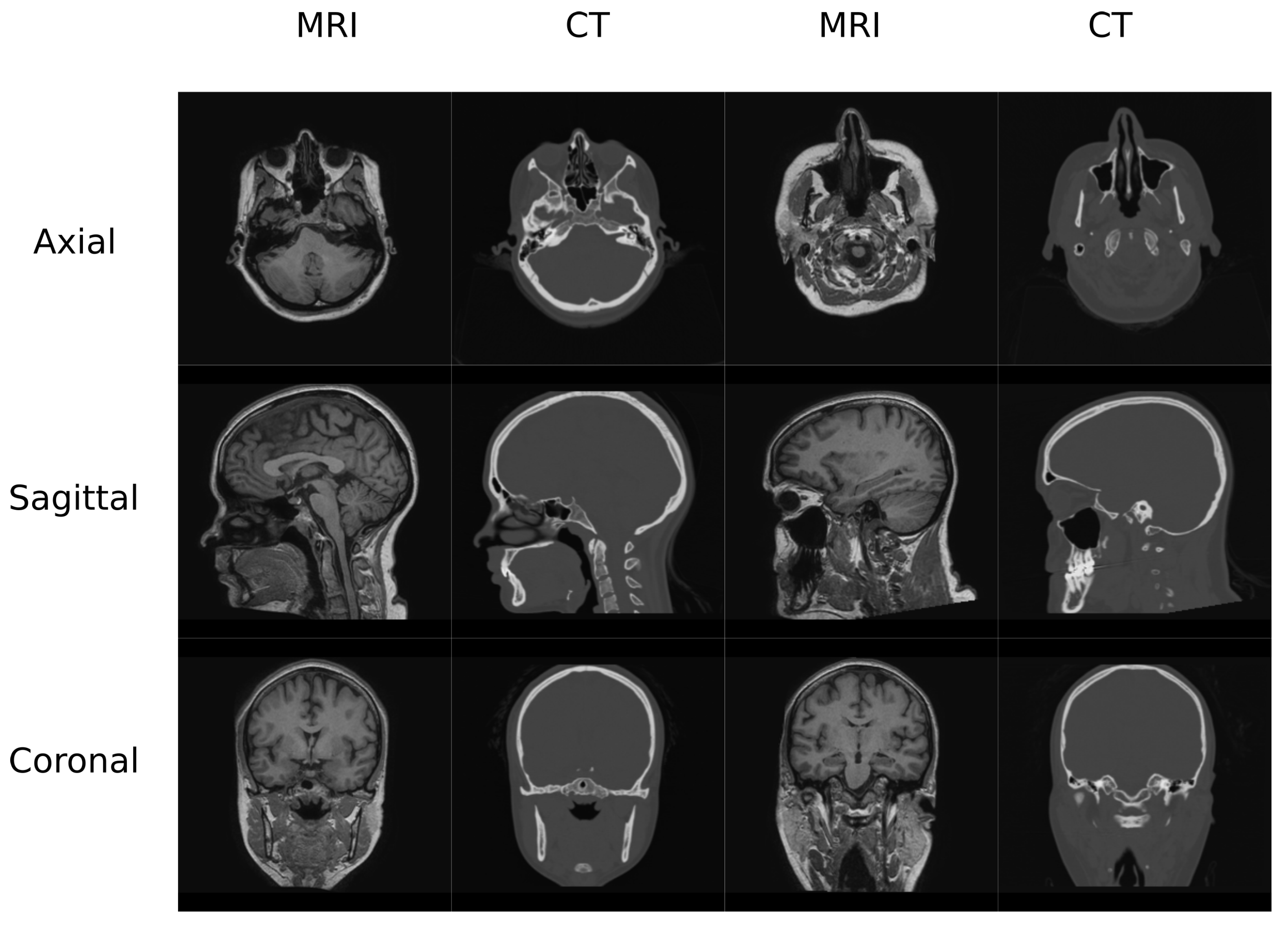
In this work, two datasets were used to train and test the different architectures that are reviewed. The first one (Figure 1) contained MR and CT head pairs from 19 healthy women (34.96 ± 5.23 y/o). MR images were acquired on a GE Signa HDxt 3.0-T MR scanner, and imaging was performed using a 3D T1-weighted sequence with a repetition time of 10.024 ms, echo time of 4.56 ms, inversion time of 600 ms, 1 excitation acquisition matrix of , isotropic 1 mm resolution, and a flip angle of 12°. Low-dose CT images were acquired on a Siemens Somatom Sensation 16 CT scanner with a matrix of , resolution of mm, slice thickness of 0.75 mm, pitch of 0.7 mm, acquisition angle of 0°, voltage of 120 kV, and radiation intensity of 200 mA.

Figure 1.
Head Data set example.
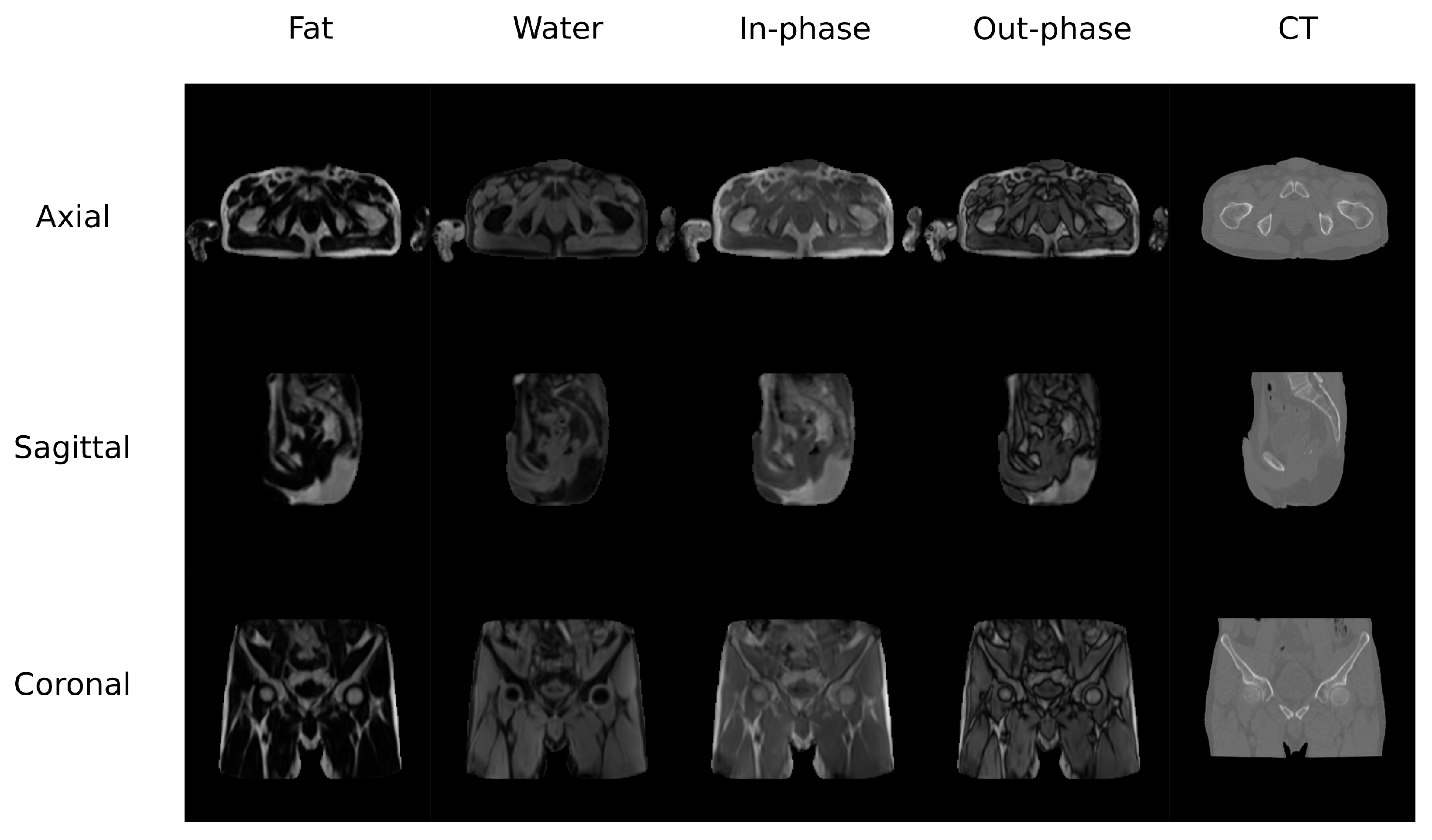
The second database (Figure 2) contained MR and CT images from the pelvis of 13 colorectal and 6 prostate cancer patients (61.42 ± 10.63 y/o, mean BMI 22.3 ± 2.88, 12 males/8 females). Additionally, images from follow-up visits for 9 of the colorectal cancer patients were also included in this study. MR and CT scans were performed on the same day with an average delay of 66 min. CT images were acquired on a Discovery PET/CT 710 scanner (GE Healthcare) with a matrix of , resolution of mm, slice thickness of 3.75 mm, pitch of 0.94 mm, acquisition angle of 0, voltage of 120 kV, and radiation intensity of 150 mA. MR data were acquired on a Biograph mMR scanner (Siemens Healthineers, Erlangen, Germany). The sequence was a dual echo Dixon-VIBE, which is the standard image for attenuation correction purposes. Dixon-Vibe acquisitions are composed by 4 sets of images: water, fat, in-phase and out-of-phase.

Figure 2.
Pelvis Data set example.
2.2. Preprocessing
The head database was preprocessed using 3D Slicer built-in modules [32,33]. The preprocessing pipeline included bias correction using the N4 algorithm, rigid registration to align the MR-CT patient pairs as well as to align all the patients in the same orientation, and histogram matching of the grayscale values. Finally, volumes were cropped to slices in the axial direction since it is easier to have a dimension which is a power of 2 in deep learning applications. This occurs due to the network operations, which half and double the spatial dimensions of the input. Figure 1 depicts examples of the volumes in this database.
The preprocesing pipeline of the pelvis dataset was composed by a bias correction performed using the N4 module in 3D Slicer followed by an intra-subject rigid and non-rigid registration using SPM8. This step is required because the pelvis is a non-rigid region and the positioning of the subject was different for the CT and MR acquisitions. The volumes were resliced and cropped to a fixed FOV of cm with mm of voxel size to ensure matrix and voxel homogeneity among subjects. This step allows to prepare the images to be suitable for the DCNN by reslicing the data to 256 voxels in the axial direction. Figure 2 shows an example of the Dixon-VIBE sequence and the corresponding CT.
2.3. Architectures
Three architectures inspired in previous works were trained and tested: Atrous-Net [25], U-Net [31] and Residual-Net [29]. These networks received MR volumes as input and generate their corresponding pseudo-CT. In the case of the head database, the input was a one-channel MR T1-weighted volume. In the pelvis database, the input was a four-channel MR Dixon-VIBE volume containing the water, fat, in-phase and out-of-phase volumes.
Each architecture described in the following subsections was implemented in two schemes: (i) using 2D convolution filters, and (ii) using 3D convolution filters. The main difference between both versions is the shape and size of the input and the number of parameters in the network. Inputs in the 2D version were axial slices of voxels with 1 or 4 channels depending on which database was used. Inputs in the 3D versions were patches with 1 or 4 channels as well depending on the database. The resulting outputs of the two versions have the same shape and size as the inputs, either a slice or a 3D patch. The reason of this size difference arises from memory limitations in the GPU used for training the networks. The 3D convolutions populate much more memory and, therefore, the input size must be reduced to a patch.
2.3.1. Atrous Net
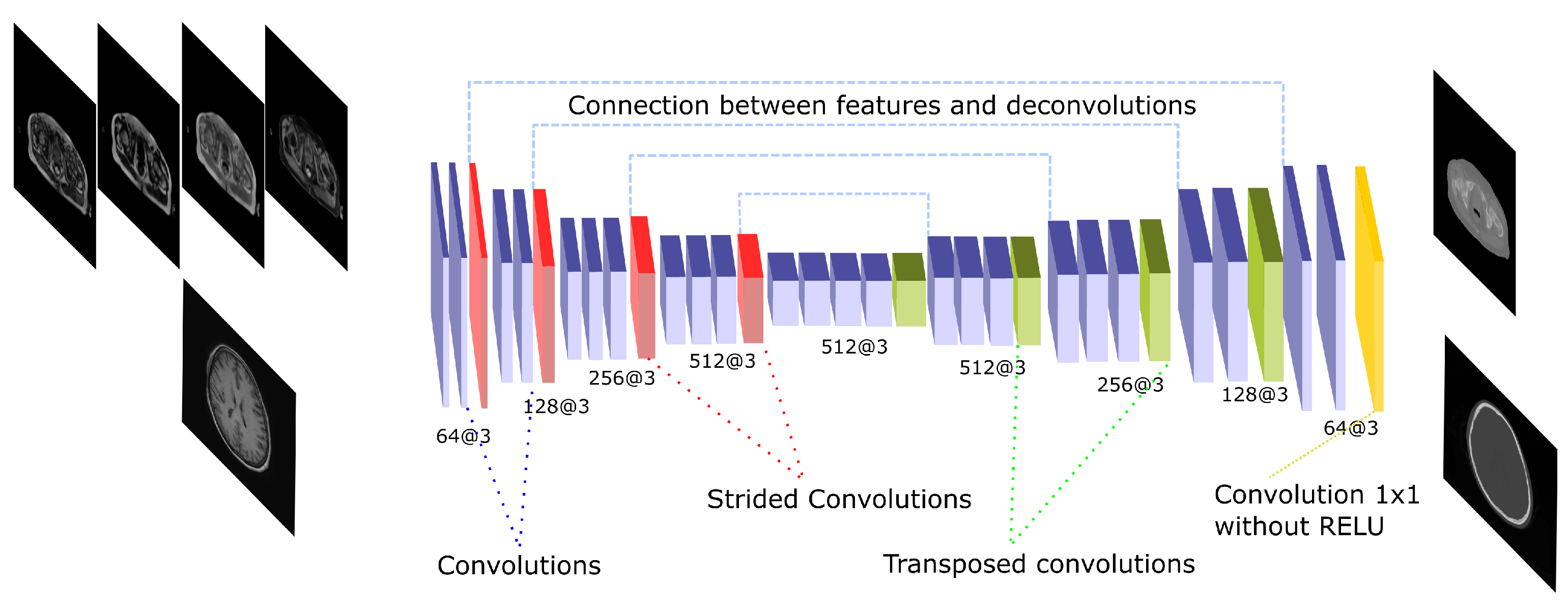
The Atrous-Net is inspired by the work by [25]. Dilated convolutions—also called atrous convolutions—are convolutional operations that are performed on non-contiguous voxels instead of being performed on adjacent voxels. The distance between voxels in a convolution is called dilation. Therefore, spatial information can be better preserved each time a filter is applied. This way, the Atrous net performs a succession of convolutions without pooling to avoid the reduction of the spatial resolution of the feature maps. It uses dilated convolutions in order to achieve enough receptive field to compute complex features. Dilated convolutions have been used with quite successful results in other works [34,35]. These convolutions are used as an alternative to the pooling operation to calculate multi-scale features without reducing the shape of the input. In this work, dilation 1 was used for the first and last layer and dilation 2 was implemented for all other layers. After every convolution, a batch normalization and a Rectified Linear Unit (ReLU) as non-linear activation are applied. Figure 3 shows a scheme of the architecture and the number of filters used in every convolution. This network performs 10 convolution operations and has 3.2 and 10.6 million parameters in the 2D and 3D implementations, respectively.
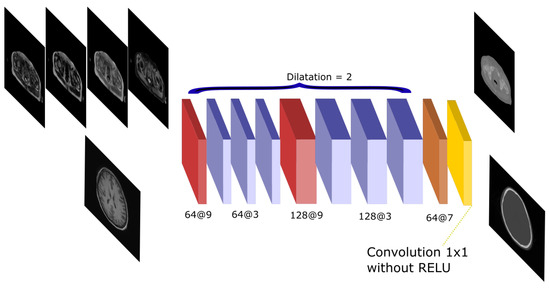
Figure 3.
Atrous-Net architecture. The scheme shows the CNN architecture including the atrous convolutions. The network receives either the four Dixon-VIBE MR sequences of the pelvis or the T1-weighted image of the brain as input. Then, it outputs a pelvis or a head pseudo-CT, respectively.
2.3.2. U-Net
The U-net architecture is a well-known network that has been used in several pseudo-CT synthesis works [21,24,30,31]. The U-net architecture is composed by an encoding step in which several convolutions and pooling operations are applied to extract a hierarchy of increasingly complex and meaningful features. Then, the features are reconstructed in a decoding step using up-sampling operations and convolutions to estimate the final output. In this work, the transposed convolution—also called fractionally strided convolution, was implemented as up-sampling operation. The transposed convolution allows the learning of parameters to perform the up-sampling, and has been previously used for pseudo-CT generation [31]. In this work, the encoding step is formed by 14 convolutions and 4 max-pooling operations. In addition, the filters are doubled after every pooling except the last one due to GPU memory restrictions. In the decoding side, 4 transposed convolutions and 10 convolutions are performed, with filters halved after every transposed convolution. An important part of the U-net is the connection between the encoding and decoding phases, which is known as skip connection. After every max-pooling operation the output is concatenated with the input of the transposed convolution in the decoding side that has the same feature size. These connections allow the decoding step to have information from different scales and feature complexity. After every convolution, a batch normalization and a ReLU activation are performed. The whole network performs 30 convolutions and contains 36.4 and 10.9 million parameters in the 2D and 3D implementations, respectively. Figure 4 depicts a scheme of this architecture.
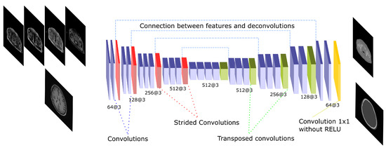
Figure 4.
U-Net architecture. The scheme shows the CNN architecture including the encoder and the decoder blocks that are linked by skip connections. The encoding part presents strided operations while the decoding part is composed by transposed convolutions. The network receives either the four Dixon-VIBE MR sequences of the pelvis or the T1-weighted image of the brain as input. Then, it outputs a pelvis or a head pseudo-CT, respectively.
2.3.3. Residual Network
The residual network is inspired in the work by [29]. The Residual network is composed by an initial convolution with a 5 × 5 kernel and two convolutions with stride 2 to reduce the input size. The filters are doubled after these strided convolutions and 9 residual blocks are applied. Finally, two transposed convolutions are performed to obtain a size equivalent to the input. The residual block is composed by several convolutions with a shortcut that adds the input of the block to the output of the last convolution in the block. Adding layers to the network usually leads to a degradation in the output. Nevertheless, the use of residual blocks allows for an increase in the number of layers (i.e., the depth of the network) without degradation [26]. The residual block used in this work is shown in Figure 5. In all convolutions, a batch normalization is applied followed by the ReLU activation function. The network has 33 convolutions composed by 16.7 and 50.7 million parameters in the 2D and 3D implementations, respectively.
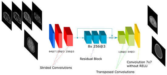
Figure 5.
Residual-Net architecture. The scheme shows the CNN architecture including the residual blocks in between the encoding and the decoding steps. The network receives either the four Dixon-VIBE MR sequences of the pelvis or the T1-weighted image of the brain as input. Then, it outputs a pelvis or a head pseudo-CT, respectively.
2.4. Common Details and Training
In order to maintain a common setup between architectures, 32 filters were used in the first convolution of every architecture. After that, depending on the specific architecture, the number of filters were doubled or halved. The mini-batch used in all architectures was 16. The optimizer chosen for training was the Adam optimizer [36] with a learning rate of , a of 0.9, a of 0.999 and an of . Adam was chosen because it is relatively easy to configure for various problems and models. The mean absolute error (MAE) between the output of the network and the ground truth CT was calculated as loss function Moreover, the weights in the network were initialized using the method described by [37] for the ReLU activation. All networks were trained until the loss is stabilised and no validation set was used because no over-fitting was found in previous experiments.
All the code used in this project was developed using the Tensorflow library. Training and testing was performed on an Nvidia GeForce RTX 2080 Ti GPU, with 11 GB of GDDR6 RAM.
2D training details: The 2D networks were trained using axial slices of shape voxels. Slices were randomly rotated as data augmentation technique. All the slices of all subjects in the training set were randomly shuffled during training, which in total add up to 4081 slices for the head dataset and 7700 slices for the pelvis dataset. To synthesize the final pseudo-CT for a subject, each slice was processed in axial order by the network. Then, the resulting pseudo-CT slices were stacked into a volume.
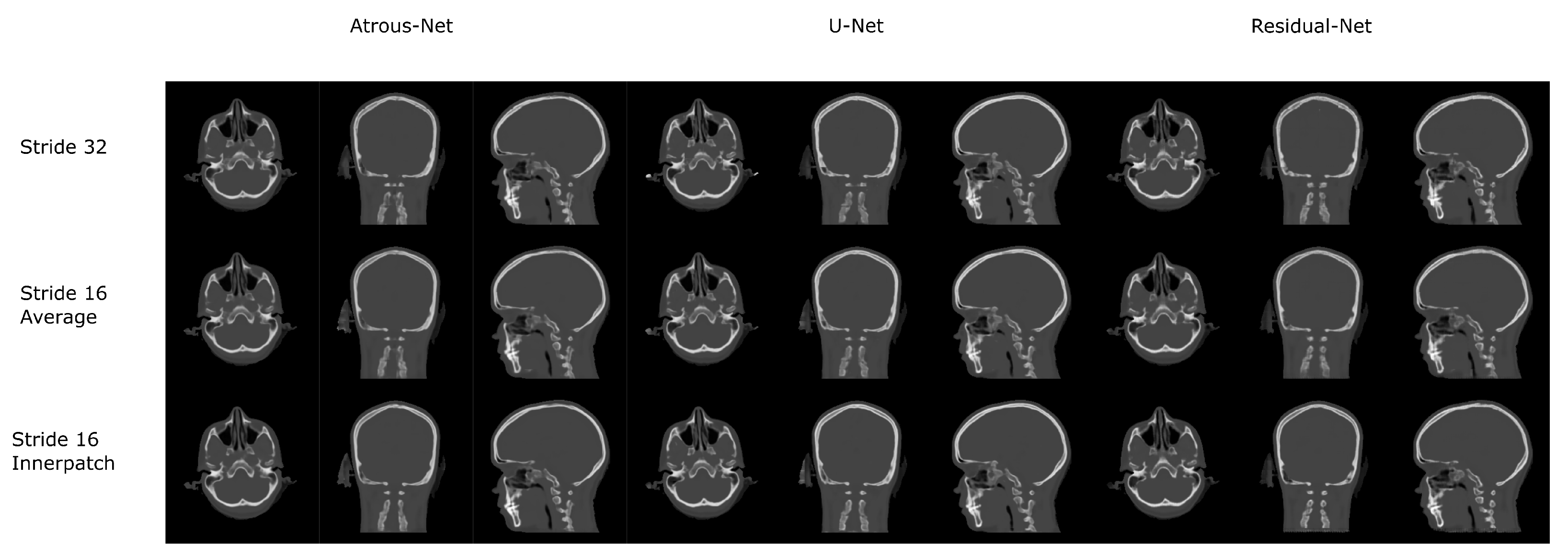
3D training details: The 3D networks were trained using 3D patches of voxels. To generate the training dataset, all possible patches that contain CT voxels were extracted using a stride of 8, which makes a total of 33,093 patches for the head and 70,554 patches for the pelvis dataset. For data augmentation, the patches were randomly rotated in the coronal and sagittal planes. During training, these 3D patches were randomly extracted from the MR and CT volumes. To obtain the pseudo-CT volume, all the patches were merged into a final volume. In this work, three different merging strategies were tested:
- The first merging approach is the simplest and it consists on extracting cubes in a sliding window of stride 32 (same as the patch size). Then, its corresponding pseudo-CT 3D patch is calculated and it is fitted into its corresponding position in the output volume.
- The second approach uses stride 16 (half patch size). It averages the overlapping voxels between patches when they are introduced in the output volume.
- The third one also consists in using stride 16, but only the center cube of the pseudo-CT 3D patch is assigned to the output volume.
The effect of these strategies in the pseudo-CT volumes are detailed in the Section 3.
Experiment details: A subject level cross-validation set-up was used to train and test all architectures with the proposed data sets. Both data sets comprised a total of 19 MR-CT subjects pairs. Thus, a 7 fold configuration was chosen, with 3 subjects in the test set and the remaining 16 for training. In the case of the pelvis dataset, several subjects had follow-up acquisitions. So it was ensured that all the volumes from a subject were taken out from training if that subject was in the test set.
Metrics: The results of every network were calculated using the outputs generated by the cross-validation. As neglecting bone, soft-tissue and fat are the main issues when synthesizing a pseudo-CT [38], we computed the results in two regions of interest: (i) the whole anatomy of the subject (including all tissues) and (ii) only the bone. To this end, a mask for soft tissue (between −100 and 100 HU), fat (lower than −100 HU) and bone (greater than 100 HU) was obtained by thresholding the Houndsfield Units (HU) in the ground truth CT. The measures calculated to compare the performance of the networks and schemes are the following:
- Mean Average Error (MAE):
- Peak Signal-to-Noise ratio (PSNR):
- Pearson Correlation Coefficient:
In Equations (1)–(4), y represents the ground truth CT voxel value and x the generated pseudo-CT voxel value. In Equation (2) the max value depicts the range of possible values for the measured signal. In our case the HU units range goes from −1024 to 3072, therefore the max range value is 4096. In the Pearson correlation coefficient, and represent the mean of the voxel values in the ground truth CT and in the pseudo-CT, respectively.
Additionally, to validate the statistical differences among the architectures and schemes, we decided to perform various statistical test over the cross-validation results. To decide which test would be the most appropriate, we tested if the results of the cross-validation tended to be Gaussian or not using a Shapiro test and a D’Agostino’s test. The results tended to be normal, thus we decided to perform several ANOVA test and Student’s t-test for paired data with a statistically significant difference defined as to verify whether certain network or scheme results were significantly different or not.
3. Results
Firstly, the results will be presented for each dataset, considering all tissues, soft-tissue, fat and bone. Each table depicts the MAE, PSNR and Pearson Coefficient results for 2D and 3D convolutions using each network architecture. For the 3D convolutions, the results for each reconstruction using stride 32 (3D-32), stride 16 with averaging (hl3D-16av) and stride 16 using the inner cube (3D-16) are depicted. Tables 15 and 30 show the time needed to synthesize a whole volume from each data set. Secondly, the results from each architecture will be reviewed separately. Finally, the results from the 3D networks using the different reconstruction strategies are presented.
3.1. Head Dataset Results
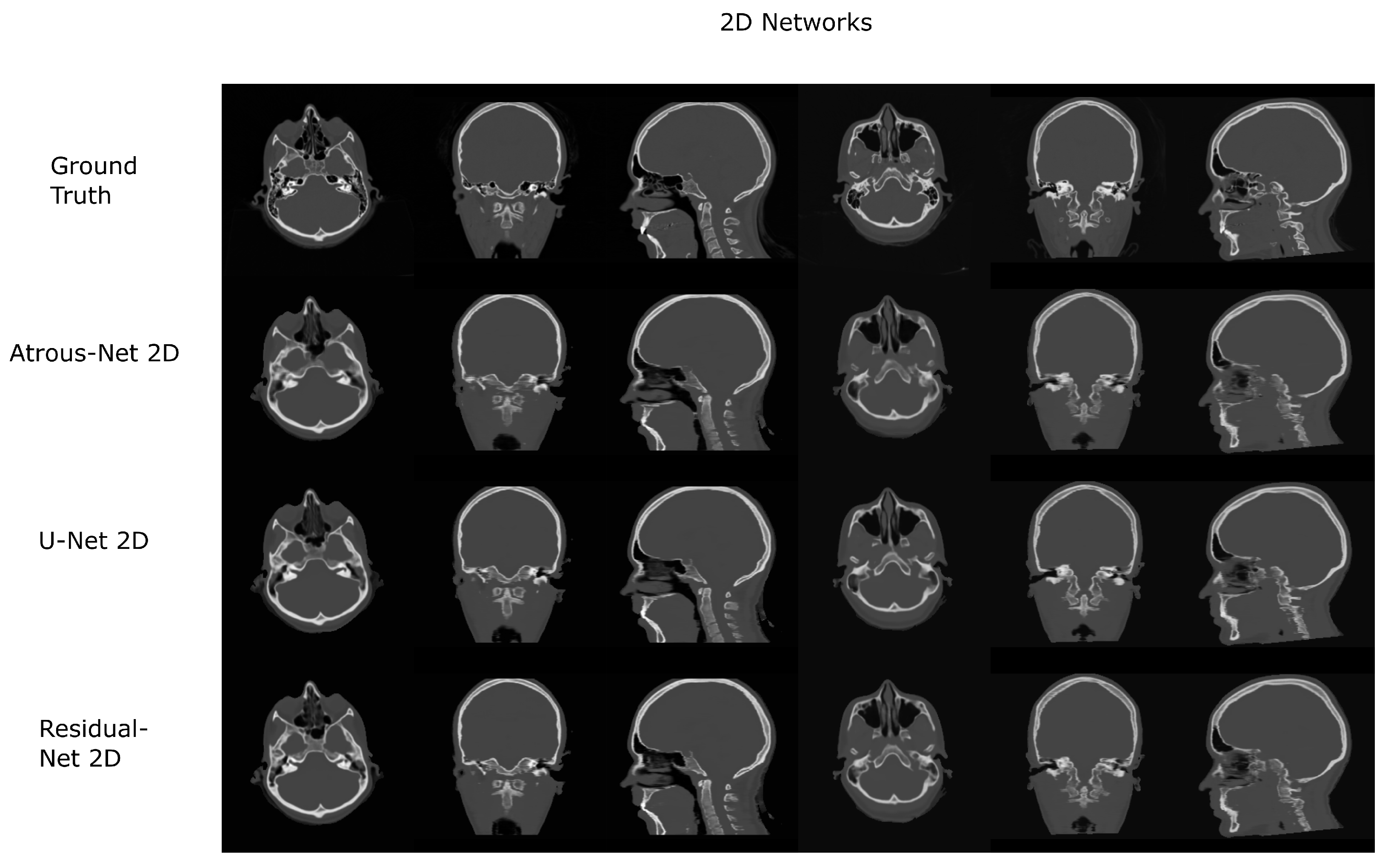
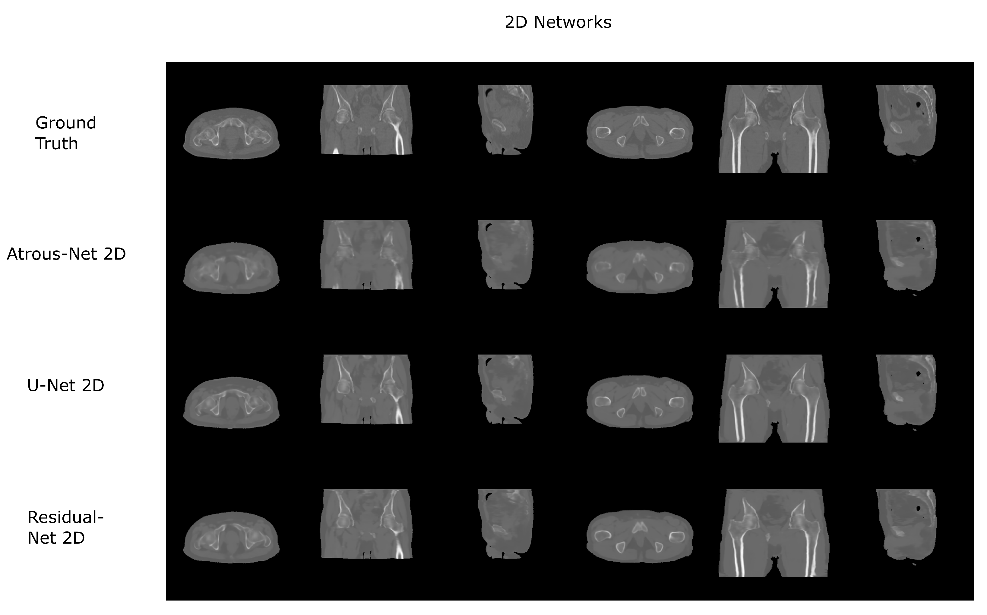
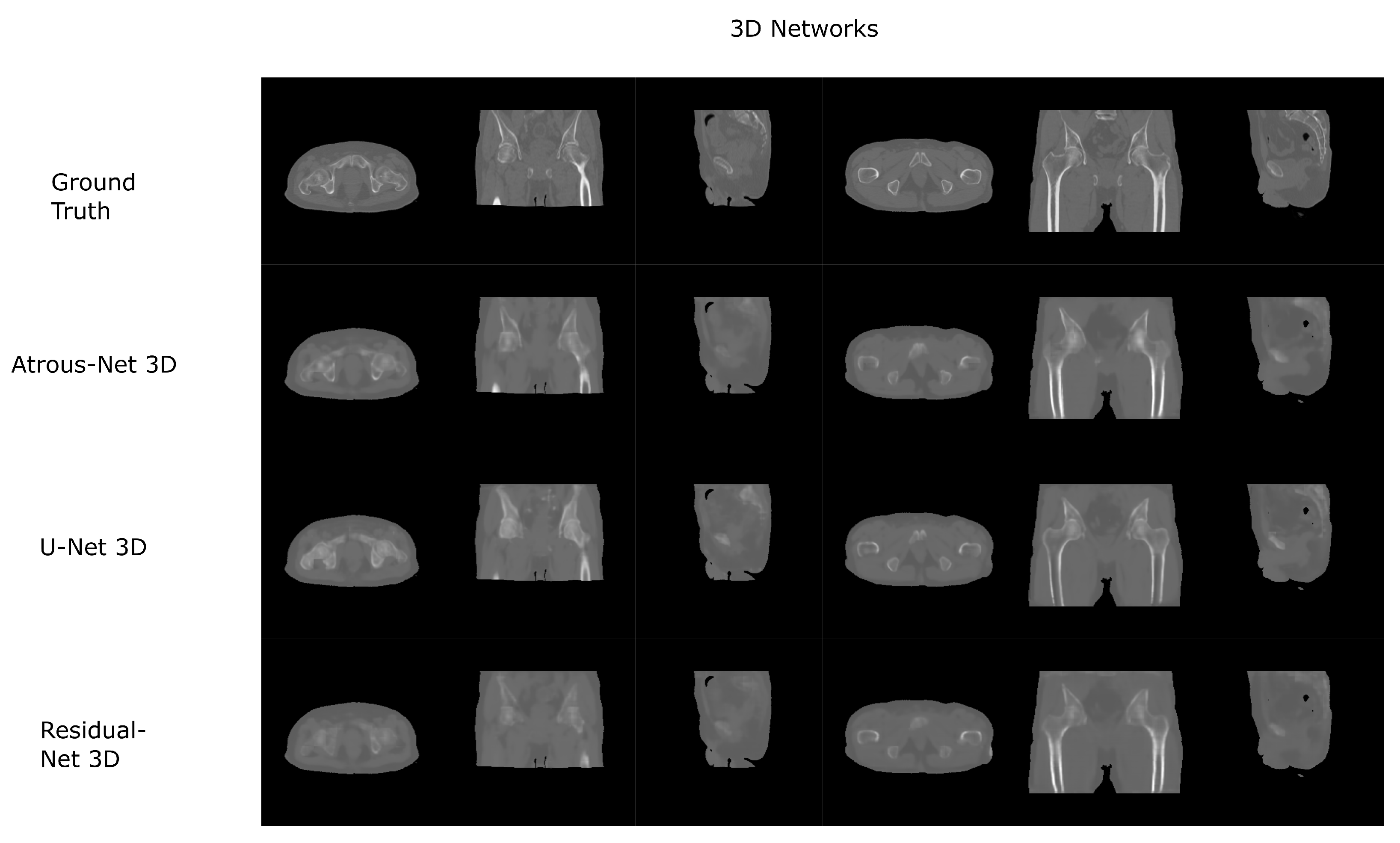
The results for all tissues using the head dataset are depicted in Table 1, Table 2 and Table 3; the results using only the bone voxels are detailed in Table 4, Table 5 and Table 6; the results using only the fat voxels are detailed in Table 7, Table 8 and Table 9; and the results using only the soft-tissue voxels are detailed in Table 10, Table 11 and Table 12. The best performing 2D network for the head dataset was the Residual-net. The results presented a MAE of 99.83 HU, a PSNR of 24.83 and a Pearson Coefficient of 0.931 in all tissues, and a MAE of 326.33 HU, a PSNR of 19.04 and a Pearson Coefficient of 0.826 in bone voxels. The ANOVA test revealed a statistically significant effect of the 2D architectures for MAE results (all tissues: , ; bone: , ) and PSNR results (all tissues: = 99.3, ; bone: = 85.6, ). A paired t-test was used to compare the Residual-net to the other networks reporting also statistically significant differences in the MAE and in the PSNR (Table 13). Using 2D convolutions, the Atrous-net and the U-net performed 5% and 18% worse than the residual-net, respectively. Moreover, the U-net network was clearly behind the other networks using 2D convolutions. Nevertheless, the U-net in 3D-16 obtained a MAE of 89.54 HU, a PSNR of 25.69 and a Pearson Coefficient of 0.943 in all tissues, and a MAE of 289.10 HU, a PSNR of 20.05 and a Pearson Coefficient of 0.861 in bone voxels, which were the best results for the head dataset. The ANOVA test also reported a statistically significant effect of the 3D networks for the MAE (all tissues: ; bone , ) and the PSNR (all tissues: , ; bone: , ). The post hoc paired t-test that is depicted in Table 14 also reported statistically significant differences in the MAE and PSNR after comparing each architecture. Summarizing, the results using 3D convolutions from the U-net were 17% and 10% better than those of the Atrous-net and Residual-net, respectively. Visual result examples of head pseudo-CTs are depicted in Figure 6 and Figure 7. Table 15 shows the time needed to synthesize a whole head volume using the different architectures.

Table 1.
Head dataset with U-net. Mean Absolute Error, PSNR and Pearson coefficient on the head data set obtained using U-net with different convolutions and reconstructions.

Table 2.
Head dataset with Atrous-Net. Mean Absolute Error, PSNR and Pearson coefficient on the head data set obtained using Atrous network with different convolutions and reconstructions.

Table 3.
Head dataset with Residual-Net. Mean Absolute Error, PSNR and Pearson coefficient on the head data set obtained using Residual net with different convolutions and reconstructions.

Table 4.
Head dataset Bone with U-net. Mean Absolute Error, PSNR and Pearson coefficient within the bone on the head data set obtained using U-net with different convolutions and reconstructions.

Table 5.
Head dataset Bone with Atrous-Net. Mean Absolute Error, PSNR and Pearson coefficient within the bone on the head data set obtained using Atrous net with different convolutions and reconstructions.

Table 6.
Head dataset Bone with Residual-Net. Mean Absolute Error, PSNR and Pearson coefficient within the bone on the head data set obtained using Residual net with different convolutions and reconstructions.

Table 7.
Head dataset Fat with U-net. Mean Absolute Error, PSNR and Pearson coefficient within the fat on the head data set obtained using U-net with different convolutions and reconstructions.

Table 8.
Head dataset Fat with Atrous-Net. Mean Absolute Error, PSNR and Pearson coefficient within the fat on the head data set obtained using Atrous network with different convolutions and reconstructions.

Table 9.
Head dataset Fat with Residual-Net. Mean Absolute Error, PSNR and Pearson coefficient within the fat on the head data set obtained using Residual net with different convolutions and reconstructions.

Table 10.
Head dataset Soft-tissue with U-net. Mean Absolute Error, PSNR and Pearson coefficient within the soft-tissue on the head data set obtained using U-net with different convolutions and reconstructions.

Table 11.
Head dataset Soft-tissue with Atrous-Net. Mean Absolute Error, PSNR and Pearson coefficient within the soft-tissue on the head data set obtained using Atrous net with different convolutions and reconstructions.

Table 12.
Head dataset Soft-tissue with Residual-Net. Mean Absolute Error, PSNR and Pearson coefficient within the bone on the head data set obtained using Residual net with different convolutions and reconstructions.

Table 13.
MAE and PSNR p-values for 2D Head. p-values of paired Student’s t-test for MAE and PSNR results with 2D architectures with the head dataset.

Table 14.
MAE and PSNR p-values for 3D Head. p-values of paired Student’s t-test for MAE and PSNR results with 3D architectures with the head dataset.

Figure 6.
Head results using 2D networks.
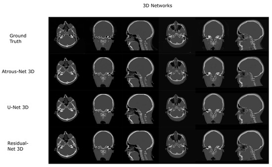
Figure 7.
Head results using 3D-16 networks.

Table 15.
Synthesis Times for Head. Average time in seconds to synthesize a whole volume from the Head data set using 2D networks and 3D networks reconstructing with stride 16 and 32.
3.2. Pelvis Dataset Results
The results for all tissues using the pelvis dataset are depicted in Table 16, Table 17 and Table 18; the results using only the bone voxels are detailed in Table 19, Table 20 and Table 21; the results using only the fat voxels are detailed in Table 22, Table 23 and Table 24; and the results using only the soft-tissue voxels are detailed in Table 25, Table 26 and Table 27. In the pelvis dataset all networks performed very similar when all tissues were considered. However, 3D networks obtained slightly worse results when assessing bone alone and very similar results for all tissues. The best network in the bone dataset was the 2D Residual network that obtained a MAE of 201.56 HU, a PSNR of 23.20 and a Pearson Coefficient of 0.476 in the bone. Additionally, the error in bone with all networks increased when the 3D scheme was used. The ANOVA test for the 2D results reported a statistically significant effect of the networks in all tissues and bone MAE (all tissues: , ; bone: , ) and PSNR (all tissues: , , bone: , ). According to 3D results, the ANOVA test did not expose statistically significant differences when using different architectures on all tissue MAE (all tissues: , ; bone: , ) and PSNR (all tissues: , ; bone: , ). Post hoc Student’s t-test is depicted in Table 28 and Table 29. It reveals that the Residual-net and Atrous-net did not provide statistically significant differences. Visual result examples of pelvis pseudo-CTs are depicted in Figure 8 and Figure 9. Table 30 shows the time needed to synthesize a whole pelvis volume using the different architectures.

Table 16.
Pelvis dataset with U-Net. Mean Absolute Error, PSNR and Pearson coefficient from U-net using different convolutions and reconstructions in the Pelvis data set.

Table 17.
Pelvis dataset with Atrous-net. Mean Absolute Error, PSNR and Pearson coefficient from Atrous-net using different convolutions and reconstructions in the Pelvis data set.

Table 18.
Pelvis dataset with Residual-net. Mean Absolute Error, PSNR and Pearson coefficient from Residual-net using different convolutions and reconstructions in the Pelvis data set.

Table 19.
Pelvis dataset Bone with U-net. Mean Absolute Error, PSNR and Pearson coefficient from U-net using different convolutions and reconstructions in the Pelvis data set within the bone.

Table 20.
Pelvis dataset Bone with Atrous-net. Mean Absolute Error, PSNR and Pearson coefficient from Atrous-net using different convolutions and reconstructions in the Pelvis data set within the bone.

Table 21.
Pelvis dataset Bone with Residual-net. Mean Absolute Error, PSNR and Pearson coefficient from Residual-net using different convolutions and reconstructions in the Pelvis data set within the bone.

Table 22.
Pelvis dataset Fat with U-Net. Mean Absolute Error, PSNR and Pearson coefficient from U-net using different convolutions and reconstructions in the Pelvis data set within the fat.

Table 23.
Pelvis dataset Fat with Atrous-net. Mean Absolute Error, PSNR and Pearson coefficient from Atrous-net using different convolutions and reconstructions in the Pelvis data set within the fat.

Table 24.
Pelvis dataset Fat with Residual-net. Mean Absolute Error, PSNR and Pearson coefficient from Residual-net using different convolutions and reconstructions in the Pelvis data set within the fat.

Table 25.
Pelvis dataset Soft-tissue with U-net. Mean Absolute Error, PSNR and Pearson coefficient from U-net using different convolutions and reconstructions in the Pelvis data set within the soft tissue.

Table 26.
Pelvis dataset Soft-tissue with Atrous-net. Mean Absolute Error, PSNR and Pearson coefficient from Atrous-net using different convolutions and reconstructions in the Pelvis data set within the soft tissue.

Table 27.
Pelvis dataset Soft-tissue with Residual-net. Mean Absolute Error, PSNR and Pearson coefficient from Residual-net using different convolutions and reconstructions in the Pelvis data set within the soft tissue.

Table 28.
MAE and PSNR p-values for 2D Pelvis. p-values of paired Student’s t-test for MAE and PSNR results with 2D architectures with the pelvis dataset.

Table 29.
MAE and PSNR p-values for 3D Pelvis. p-values of paired Student’s t-test for MAE and PSNR results with 3D architectures with the pelvis dataset.
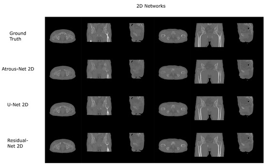
Figure 8.
Pelvis results using 2D networks.
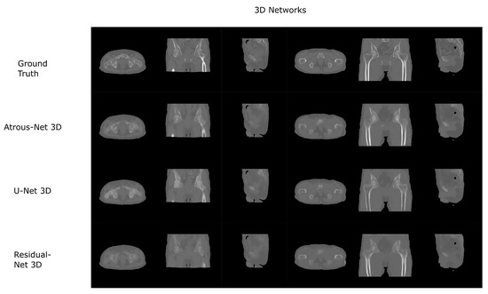
Figure 9.
Pelvis results using 3D-16 networks.

Table 30.
Synthesis Times for Pelvis. Average time in seconds to synthesize a whole volume from the Pelvis Dataset using 2D networks and 3D networks reconstructing with stride 16 and 32.
3.3. Network Architecture Results
3.3.1. Atrous-Net Results
The Atrous-net obtained a MAE of 105.16 HU in head bone and a MAE of 210.51 HU in pelvis bone. In the head dataset, this result was 18% worse than the best result. In pelvis, it was around 5% worse. The Atrous-net showed not statistically significant differences in pelvis between 2D and 3D MAE (all tissues: , ; bone: , ) and PSNR (all tissues: , ; bone: , ). However, for the head data set there were statistically significant differences in bone depiction between 2D and 3D MAE (all tissues: , , bone: , ) and PSNR (all tissues: , ; bone: , ).
3.3.2. U-Net Results
The 3D U-net architecture obtained a MAE of 89.54 HU, a PSNR of 25.69 and a Pearson Coefficient of 0.943 in the head dataset, which is the best result obtained for this dataset. However, the 2D scheme obtained a poor result of 117.21 HU for MAE, 23.26 for PSNR and 0.898 for Pearson coefficient in the head, being far away from the other two networks using 2D filters. According to the pelvis dataset, the 3D U-net obtained the best result among the 3D networks. Even so, it was around 1% worse than the best result for this dataset. Focusing on the 3D results, the U-net always had the best performance in both datasets. However, in the pelvis dataset, the U-net obtained a similar performance with statistically significant differences between the 2D and 3D MAE (all tissues: , , bone: , ) but not for PSNR (all tissues: = 1.3, ; bone: , ). In addition, the 2D scheme was slightly better for bone estimation.
3.3.3. Residual-Net Results
The residual network that was obtained for the head dataset showed statistically significant differences between the 2D and 3D schemes for bone MAE (all tissues: , ; bone: , ). However, for bone PSNR (all tissues: , ), bone: , ) there was not any statistically significant difference. In the head dataset, the 3D-16av scheme showed the minor error for bone calculations. Nevertheless, the U-net provided better results with lower errors. In the pelvis dataset, the 2D Residual-net provided the best results for bone calculations: MAE = 201.56 HU, PSNR = 23.20 and Pearson coefficient = 0.476.
3.4. 3D Reconstruction Results
Figure 10 and Figure 11 show the results of the three merging strategies that have been tested: stride 32, stride 16 with averaging of overlapping voxels and stride 16 considering the inner cube. The average time to synthesize a volume is shown in Table 15 and Table 30. The first method—referred as “stride 32” in Figure 10 and Figure 11—generated artifacts in the boundaries of the cube and misalignment in the bone and air structures. Moreover, this approach showed a greater error than the other two in the quantitative results. Nevertheless, this method was quite fast, generating a volume in 8–19 s. The other two methods provided, in average, a similar quantitative result, being the use of the inner cube slightly better. However, the use of stride 16 increased the time to generate a pseudo-CT volume up to 58–90 s. According to the averaging strategy, some artifacts can be noticed in the boundaries of the cubes after a visual inspection of the results.
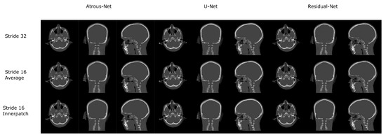
Figure 10.
Comparison between the reconstruction method proposed.
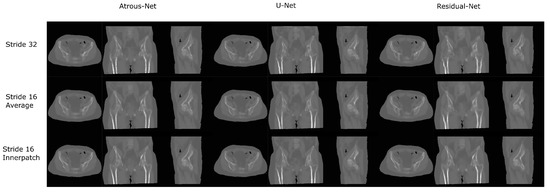
Figure 11.
Comparison between the reconstruction method proposed.
4. Discussion
Before this study, several proposals for synthesizing pseudo-CT from MR data with deep learning approaches have been published. They have demonstrated different advantages of deep learning over the previous state of the art. The most important advantages of deep learning approaches are: the capability of accommodating larger training datasets, a faster computation time when the network is deployed, the lack of the need for a registration to a common space once the model is trained, and a lower error in the generated pseudo-CT. However, the lack of a common database among research groups makes hard to assess which architecture or strategy would be the best to apply in the future. In this work, different architectures using 2D and 3D approaches were tested on two different datasets. This way, it is possible to extract conclusions when different networks are compared with the same datasets. The datasets utilized in this study were composed of 3D T1-weighted MR images of the head and Dixon-VIBE MR images of the pelvis.
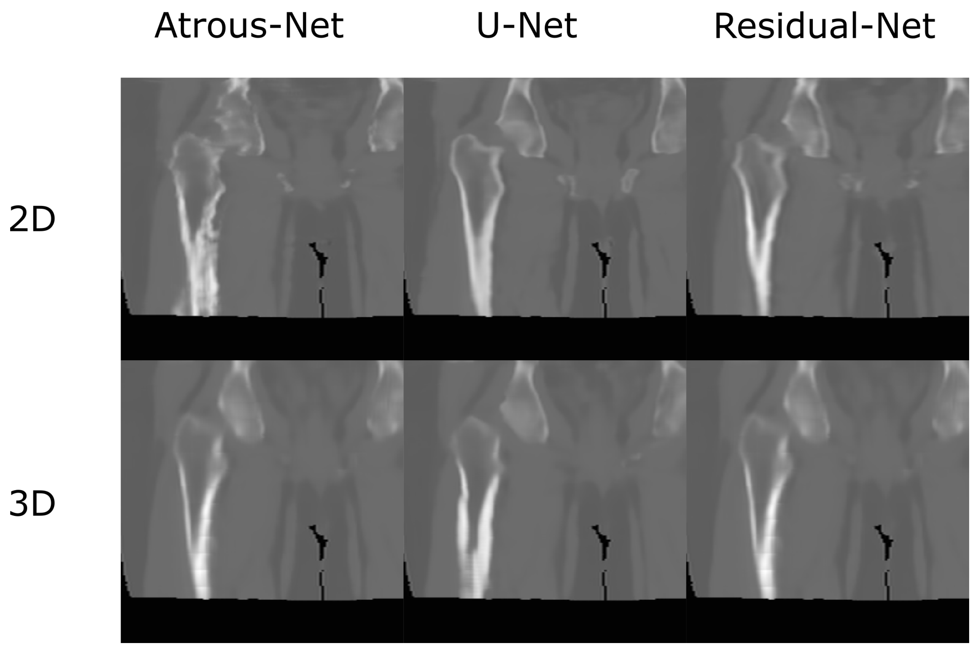
According to the results of the current work, there is no preferred network for every problem. Thus, the results depend on the specific anatomy defining the problem and the MRI sequence that is used. As shown in Section 4. Results, if the anatomy is similar to a head with complex bone structures and geometries, 2D schemes generate aliasing and artifacts across bone structures. Instead, 3D schemes and reconstructions with stride 16 provide bones with smooth boundaries, which is translated into a significant reduction of the error. Moreover, the best architecture to achieve the best detail in a head pseudo-CT is the 3D U-net (). When using 3D architectures, the input of the network is usually a 3D patch due to GPU memory limitations. 3D patches only depict a part of the anatomy. Therefore, they provide limited contextual information. In this case, the progressive spatial reduction and up-sampling of the feature maps are probably the best option, as it occurs in the U-net.
In case the anatomy does not have complex structures across slices, 3D schemes are not the best option. Moreover, if the input image has very similar areas -as in pelvis acquisitions-, 3D patches will not satisfactory synthesize the pseudo-CT due to the lack of contextual information. In this scenario, according to our results, it would be better to use a 2D scheme. Specifically, the residual network obtained the best results in 2D (), which is consistent with the results in general computer vision, where 2D approaches are used [26,39].
The dilated network did not stand out in any dataset but in the 2D scheme it performed similarly to the residual network. Nevertheless, dilated convolutions have been reported to give interesting results in segmentation in other areas of computer vision. Thus, their accommodation in an architecture in the future could improve the quality of the synthesized image.
In the pelvis dataset, the results were quite similar between networks, having differences in a range of 5% in the bone. This could be due to the input data used in the experiment: the Dixon-VIBE MRI. The Dixon-VIBE, as shown in Figure 2, does not depict the bone well. Moreover, it is fairly probable that the information to generate the pseudo-CT that it is contained in the image is low or moderate compared to T1 acquisitions (see Figure 1). That is, the networks gave similar results because the information that can be extracted from the input images is limited. However, Dixon-VIBE is the standard acquisition in PET attenuation correction and it is usually easier to have access to this type of acquisitions for the pelvis anatomy. Therefore, the type of network that is implemented does not have a great impact on the results.
In this work, different ways of reconstructing pseudo-CT volumes from 3D patches were evaluated as well. According to our results, the best option would consist in using stride 16 and the inner cube of the patch. Compared to the averaging technique, the quantitative results were similar but the visual results (Figure 12 and Figure 13) showed less artifacts and aliasing effect in the boundaries of the patches when the inner patch is used. The only reason to use a direct merge of the patches using stride 32 would be real-time applications in which a fast reconstruction of the volumes is needed. However, the stride 16 scheme took around one minute to complete a volume, which is fairly low compared to acquisition times in MRI.
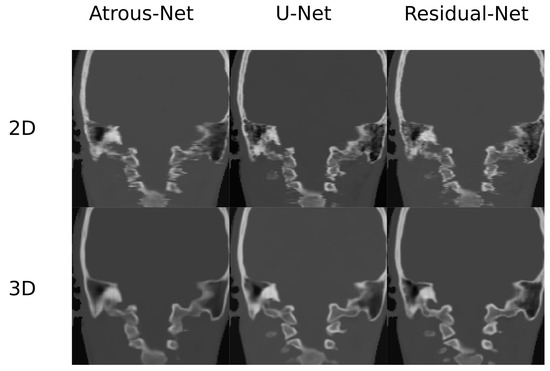
Figure 12.
Comparison in the sagittal and coronal direction for the head between the 2D and 3D schemes.

Figure 13.
Comparison in the sagittal and coronal direction for the pelvis between the 2D and 3D schemes.
Finally, it is important to mention the main limitations of this study. Firstly, the architectures that were implemented are not exactly the same as the original ones and they lack some post-processing, such as the adversarial scheme. Moreover, it is hard to verify the reproducibility and robustness of the methods compared to traditional approaches. Thus, there exists a need of a specific training dataset for scans from different vendors or field strengths [40]. Likewise, a common dataset would be useful to compare novel architectures to the state-of-the-art methods. In addition, there exist some limitations during network training due to RAM (Random Access Memory) memory restrictions. A larger memory would enable the algorithm to admit the whole volumes as input without the need of using 2D slices or 3D patches. This way, the efficiency of the DCNN would increase and better results could be obtained. Finally, using datasets with larger cohorts could also help improve the quality of the resulting pseudo-CTs.
In summary, 3D networks would be the best option if a GPU with enough memory to accommodate a whole 3D volume or at least a bigger 3D patch. A GPU with 11 GB of memory was used for this study. Nevertheless, recently, Nvidia released a new GPU with 24 GB of RAM that could help in these tasks. In addition, building a network that adds up the best qualities of the present networks is also encouraged. A U-net with residual blocks and dilated convolutions in the middle could be a good starting point. This network could exploit the progressive reduction of the feature maps and increase the value of the features using residual and dilated convolutions.
5. Conclusions
Taking into account the anatomy from which the pseudo-CTs are synthesized is extremely important to choose a specific deep learning architecture, as it has been demonstrated in this work. The first conclusion that has been extracted from this work is the importance of bone structures in the input volumes. The 3D scheme works better if the bone presents complex structures across the slices. The loss of context information for the use of 3D patches is compensated by a smoother bone depiction in the result. Instead, if the bone does not vary across slices, such as in pelvic anatomies, it is better to use a slice-by-slice strategy with 2D filters.
Moreover, the current results indicate that the 3D U-net gives better results than other strategies, such as residuals or dilated convolutions. Therefore, a U-net would be the best option to build a 3D architecture due to the progressive down-sampling and up-sampling of the feature maps. In case a 2D input is used, the best option would be a network to extract complex features, such as the residual network that is presented in this paper.
Therefore, according to these results, architectures that perform an aggressive sub-sampling, using strided convolutions or pooling operations, are quite successful if the input has a large enough field of view. Besides, the residuals work better with 2D inputs due to the limitations in the GPU memory, which do not allow to have big enough networks to extract highly processed features in 3D schemes.
Finally, the importance of the MRI sequence that is used as input in pelvis reconstructions must be remarked. The Dixon-Vibe MRI is the usual sequence acquired in the clinic. However, it probably does not contain enough information for pseudo-CT generation, given the similar results between the evaluated networks and schemes. Hence, in future works it would be interesting to compare results with Dixon-VIBE, T1 or even the recent zero-echo-time acquisitions using a DCNN.
Author Contributions
Conceptualization, J.V.-O., A.T.-C., D.I.-G. and N.M.; Data curation, A.T.-C. and C.P.-d.-l.-L.; Formal Analysis, J.V.-O. and A.T.-C.; Funding acquisition, A.T.-C., Y.R. and N.M.; Investigation, J.V.-O., A.T.-C. and C.P.-d.-l.-L.; Methodology, J.V.-O., A.T.-C., C.P.-d.-l.-L., D.I.-G. and N.M.; Resources, A.T.-C., O.A.C., Y.R., F.M., A.S., M.S., D.I.-G. and N.M.; Software, J.V.-O. and A.T.-C.; Supervision, A.T.-C., D.I.-G. and N.M.; Validation, J.V.-O., A.T.-C. and C.P.-d.-l.-L.; Visualization, J.V.-O., A.T.-C. and C.P.-d.-l.-L., Writing—original draft preparation, J.V.-O. and A.T.-C., C.P.-d.-l.-L., D.I.-G. and N.M.; writing—review and editing, J.V.-O., A.T.-C., C.P.-d.-l.-L., O.A.C., Y.R., F.M., A.S., M.S., D.I.-G. and N.M. All authors have read and agreed to the published version of the manuscript.
Funding
This project was partially supported by Young Reserchers R&D Project Ref M2166 (MIMC3-PET/MR) financed by Community of Madrid and Rey Juan Carlos University and by project DPI2015-68664-C4-2-R of the Spanish Ministry of Economy and by Banco de Santander and Universidad Rey Juan Carlos Funding Program for Excellence Research Groups ref. “Computer Vision and Image Processing (CVIP)”.
Institutional Review Board Statement
The study was conducted in accordance with the Declaration of Helsinki. The data analysis was approved by the Partners Healthcare Ethics Committee (SDN-Pascale IRB-CODE No.1/16-16-03-16).
Informed Consent Statement
Patient consent was waived due to the retrospective nature of this study.
Conflicts of Interest
The authors declare no conflict of interest.
References
- Burger, C.; Goerres, G.; Schoenes, S.; Buck, A.; Lonn, A.; Von Schulthess, G. PET attenuation coefficients from CT images: Experimental evaluation of the transformation of CT into PET 511-keV attenuation coefficients. Eur. J. Nucl. Med. Mol. Imaging 2002, 29, 922–927. [Google Scholar] [CrossRef] [PubMed]
- Shao, Y.; Cherry, S.R.; Farahani, K.; Meadors, K.; Siegel, S.; Silverman, R.W.; Marsden, P.K. Simultaneous PET and MR imaging. Phys. Med. Biol. 1997, 42, 1965. [Google Scholar] [CrossRef]
- Martinez-Möller, A.; Souvatzoglou, M.; Delso, G.; Bundschuh, R.A.; Chefd’hotel, C.; Ziegler, S.I.; Navab, N.; Schwaiger, M.; Nekolla, S.G. Tissue classification as a potential approach for attenuation correction in whole-body PET/MRI: Evaluation with PET/CT data. J. Nucl. Med. 2009, 50, 520–526. [Google Scholar] [CrossRef] [PubMed]
- Hu, Z.; Ojha, N.; Renisch, S.; Schulz, V.; Torres, I.; Buhl, A.; Pal, D.; Muswick, G.; Penatzer, J.; Guo, T.; et al. MR-based attenuation correction for a whole-body sequential PET/MR system. In Proceedings of the 2009 IEEE Nuclear Science Symposium Conference Record (NSS/MIC), Orlando, FL, USA, 25–31 October 2009; IEEE: Piscataway, NJ, USA, 2009; pp. 3508–3512. [Google Scholar]
- Wagenknecht, G.; Kaiser, H.J.; Mottaghy, F.M.; Herzog, H. MRI for attenuation correction in PET: Methods and challenges. Magn. Reson. Mater. Phys. Biol. Med. 2013, 26, 99–113. [Google Scholar] [CrossRef]
- Izquierdo-Garcia, D.; Sawiak, S.J.; Knesaurek, K.; Narula, J.; Fuster, V.; Machac, J.; Fayad, Z.A. Comparison of MR-based attenuation correction and CT-based attenuation correction of whole-body PET/MR imaging. Eur. J. Nucl. Med. Mol. Imaging 2014, 41, 1574–1584. [Google Scholar] [CrossRef] [PubMed]
- Berker, Y.; Franke, J.; Salomon, A.; Palmowski, M.; Donker, H.C.; Temur, Y.; Mottaghy, F.M.; Kuhl, C.; Izquierdo-Garcia, D.; Fayad, Z.A.; et al. MRI-based attenuation correction for hybrid PET/MRI systems: A 4-class tissue segmentation technique using a combined ultrashort-echo-time/Dixon MRI sequence. J. Nucl. Med. 2012, 53, 796–804. [Google Scholar] [CrossRef]
- Hsu, S.H.; Cao, Y.; Huang, K.; Feng, M.; Balter, J.M. Investigation of a method for generating synthetic CT models from MRI scans of the head and neck for radiation therapy. Phys. Med. Biol. 2013, 58, 8419. [Google Scholar] [CrossRef]
- Zheng, W.; Kim, J.P.; Kadbi, M.; Movsas, B.; Chetty, I.J.; Glide-Hurst, C.K. Magnetic resonance–based automatic air segmentation for generation of synthetic computed tomography scans in the head region. Int. J. Radiat. Oncol. Biol. Phys. 2015, 93, 497–506. [Google Scholar] [CrossRef] [PubMed]
- Ladefoged, C.N.; Benoit, D.; Law, I.; Holm, S.; Kjær, A.; Højgaard, L.; Hansen, A.E.; Andersen, F.L. Region specific optimization of continuous linear attenuation coefficients based on UTE (RESOLUTE): Application to PET/MR brain imaging. Phys. Med. Biol. 2015, 60, 8047. [Google Scholar] [CrossRef]
- Izquierdo-Garcia, D.; Hansen, A.E.; Förster, S.; Benoit, D.; Schachoff, S.; Fürst, S.; Chen, K.T.; Chonde, D.B.; Catana, C. An SPM8-based approach for attenuation correction combining segmentation and nonrigid template formation: Application to simultaneous PET/MR brain imaging. J. Nucl. Med. 2014, 55, 1825–1830. [Google Scholar] [CrossRef]
- Merida, I.; Costes, N.; Heckemann, R.; Hammers, A. Pseudo-CT generation in brain MR-PET attenuation correction: Comparison of several multi-atlas methods. In Proceedings of the EJNMMI Physics, Biodola, Italy, 17–21 May 2015; SpringerOpen: New York, NY, USA, 2015; Volume 2, p. 1. [Google Scholar]
- Burgos, N.; Cardoso, M.J.; Thielemans, K.; Modat, M.; Pedemonte, S.; Dickson, J.; Barnes, A.; Ahmed, R.; Mahoney, C.J.; Schott, J.M.; et al. Attenuation correction synthesis for hybrid PET-MR scanners: Application to brain studies. IEEE Trans. Med. Imaging 2014, 33, 2332–2341. [Google Scholar] [CrossRef] [PubMed]
- Uh, J.; Merchant, T.E.; Li, Y.; Li, X.; Hua, C. MRI-based treatment planning with pseudo CT generated through atlas registration. Med. Phys. 2014, 41, 051711. [Google Scholar] [CrossRef] [PubMed]
- Torrado-Carvajal, A.; Herraiz, J.L.; Alcain, E.; Montemayor, A.S.; Garcia-Cañamaque, L.; Hernandez-Tamames, J.A.; Rozenholc, Y.; Malpica, N. Fast patch-based pseudo-CT synthesis from T1-weighted MR images for PET/MR attenuation correction in brain studies. J. Nucl. Med. 2016, 57, 136–143. [Google Scholar] [CrossRef] [PubMed]
- Sjölund, J.; Forsberg, D.; Andersson, M.; Knutsson, H. Generating patient specific pseudo-CT of the head from MR using atlas-based regression. Phys. Med. Biol. 2015, 60, 825. [Google Scholar] [CrossRef]
- Torrado-Carvajal, A.; Herraiz, J.L.; Hernandez-Tamames, J.A.; San Jose-Estepar, R.; Eryaman, Y.; Rozenholc, Y.; Adalsteinsson, E.; Wald, L.L.; Malpica, N. Multi-atlas and label fusion approach for patient-specific MRI based skull estimation. Magn. Reson. Med. 2016, 75, 1797–1807. [Google Scholar] [CrossRef]
- Kapanen, M.; Tenhunen, M. T1/T2*-weighted MRI provides clinically relevant pseudo-CT density data for the pelvic bones in MRI-only based radiotherapy treatment planning. Acta Oncol. 2013, 52, 612–618. [Google Scholar] [CrossRef]
- Johansson, A.; Garpebring, A.; Karlsson, M.; Asklund, T.; Nyholm, T. Improved quality of computed tomography substitute derived from magnetic resonance (MR) data by incorporation of spatial information–potential application for MR-only radiotherapy and attenuation correction in positron emission tomography. Acta Oncol. 2013, 52, 1369–1373. [Google Scholar] [CrossRef]
- Navalpakkam, B.K.; Braun, H.; Kuwert, T.; Quick, H.H. Magnetic resonance–based attenuation correction for PET/MR hybrid imaging using continuous valued attenuation maps. Investig. Radiol. 2013, 48, 323–332. [Google Scholar] [CrossRef]
- Han, X. MR-based synthetic CT generation using a deep convolutional neural network method. Med. Phys. 2017, 44, 1408–1419. [Google Scholar] [CrossRef]
- Ronneberger, O.; Fischer, P.; Brox, T. U-net: Convolutional networks for biomedical image segmentation. In Proceedings of the International Conference on Medical Image Computing and Computer-Assisted Intervention, Munich, Germany, 5–9 October 2015; Springer: Berlin/Heidelberg, Germany, 2015; pp. 234–241. [Google Scholar]
- Han, X. TU-AB-BRA-02: An Efficient Atlas-Based Synthetic CT Generation Method. Med. Phys. 2016, 43, 3733. [Google Scholar] [CrossRef]
- Liu, F.; Jang, H.; Kijowski, R.; Bradshaw, T.; McMillan, A.B. Deep learning MR imaging–based attenuation correction for PET/MR imaging. Radiology 2017, 286, 676–684. [Google Scholar] [CrossRef] [PubMed]
- Nie, D.; Trullo, R.; Lian, J.; Wang, L.; Petitjean, C.; Ruan, S.; Wang, Q.; Shen, D. Medical image synthesis with deep convolutional adversarial networks. IEEE Trans. Biomed. Eng. 2018, 65, 2720–2730. [Google Scholar] [CrossRef] [PubMed]
- He, K.; Zhang, X.; Ren, S.; Sun, J. Deep residual learning for image recognition. In Proceedings of the IEEE Conference on Computer Vision and Pattern Recognition, Las Vegas, NV, USA, 27–30 June 2016; pp. 770–778. [Google Scholar]
- Tu, Z.; Bai, X. Auto-context and its application to high-level vision tasks and 3d brain image segmentation. IEEE Trans. Pattern Anal. Mach. Intell. 2009, 32, 1744–1757. [Google Scholar]
- Goodfellow, I.; Pouget-Abadie, J.; Mirza, M.; Xu, B.; Warde-Farley, D.; Ozair, S.; Courville, A.; Bengio, Y. Generative adversarial nets. In Proceedings of the Advances in Neural Information Processing Systems, Montreal, QC, Canada, 8–13 December 2014; pp. 2672–2680. [Google Scholar]
- Emami, H.; Dong, M.; Nejad-Davarani, S.P.; Glide-Hurst, C.K. Generating synthetic CTs from magnetic resonance images using generative adversarial networks. Med. Phys. 2018, 45, 3627–3636. [Google Scholar] [CrossRef]
- Leynes, A.P.; Yang, J.; Wiesinger, F.; Kaushik, S.S.; Shanbhag, D.D.; Seo, Y.; Hope, T.A.; Larson, P.E. Zero-echo-time and Dixon deep pseudo-CT (ZeDD CT): Direct generation of pseudo-CT images for pelvic PET/MRI attenuation correction using deep convolutional neural networks with multiparametric MRI. J. Nucl. Med. 2018, 59, 852–858. [Google Scholar] [CrossRef]
- Torrado-Carvajal, A.; Vera-Olmos, J.; Izquierdo-Garcia, D.; Catalano, O.A.; Morales, M.A.; Margolin, J.; Soricelli, A.; Salvatore, M.; Malpica, N.; Catana, C. Dixon-VIBE deep learning (DIVIDE) pseudo-CT synthesis for pelvis PET/MR attenuation correction. J. Nucl. Med. 2019, 60, 429–435. [Google Scholar] [CrossRef]
- Fedorov, A.; Beichel, R.; Kalpathy-Cramer, J.; Finet, J.; Fillion-Robin, J.C.; Pujol, S.; Bauer, C.; Jennings, D.; Fennessy, F.; Sonka, M.; et al. 3D Slicer as an image computing platform for the Quantitative Imaging Network. Magn. Reson. Imaging 2012, 30, 1323–1341. [Google Scholar] [CrossRef]
- Kikinis, R.; Pieper, S.D.; Vosburgh, K.G. 3D Slicer: A platform for subject-specific image analysis, visualization, and clinical support. In Intraoperative Imaging and Image-Guided Therapy; Springer: Berlin/Heidelberg, Germany, 2014; pp. 277–289. [Google Scholar]
- Chen, L.C.; Papandreou, G.; Kokkinos, I.; Murphy, K.; Yuille, A.L. Deeplab: Semantic image segmentation with deep convolutional nets, atrous convolution, and fully connected crfs. IEEE Trans. Pattern Anal. Mach. Intell. 2017, 40, 834–848. [Google Scholar] [CrossRef]
- Chen, L.C.; Papandreou, G.; Schroff, F.; Adam, H. Rethinking atrous convolution for semantic image segmentation. arXiv 2017, arXiv:1706.05587. [Google Scholar]
- Kingma, D.P.; Ba, J. Adam: A method for stochastic optimization. arXiv 2014, arXiv:1412.6980. [Google Scholar]
- He, K.; Zhang, X.; Ren, S.; Sun, J. Delving deep into rectifiers: Surpassing human-level performance on imagenet classification. In Proceedings of the IEEE International Conference on Computer Vision, Santiago, Chile, 7–13 December 2015; pp. 1026–1034. [Google Scholar]
- Mérida, I.; Costes, N.; Heckemann, R.A.; Drzezga, A.; Förster, S.; Hammers, A. Evaluation of several multi-atlas methods for PSEUDO-CT generation in brain MRI-PET attenuation correction. In Proceedings of the 2015 IEEE 12th International Symposium on Biomedical Imaging (ISBI), New York, NY, USA, 16–19 April 2015; IEEE: Piscataway, NJ, USA, 2015; pp. 1431–1434. [Google Scholar]
- Chollet, F. Xception: Deep learning with depthwise separable convolutions. In Proceedings of the IEEE Conference on Computer Vision and Pattern Recognition, Honolulu, HI, USA, 21–26 July 2017; pp. 1251–1258. [Google Scholar]
- Izquierdo-Garcia, D.; Eldaief, M.C.; Vangel, M.G.; Catana, C. Intrascanner reproducibility of an SPM-based head MR-based attenuation correction method. IEEE Trans. Radiat. Plasma Med. Sci. 2018, 3, 327–333. [Google Scholar] [CrossRef] [PubMed]
Publisher’s Note: MDPI stays neutral with regard to jurisdictional claims in published maps and institutional affiliations. |
© 2022 by the authors. Licensee MDPI, Basel, Switzerland. This article is an open access article distributed under the terms and conditions of the Creative Commons Attribution (CC BY) license (https://creativecommons.org/licenses/by/4.0/).

