Abstract
It is challenging to plan paths for autonomous vehicles on half-structured roads because of the vast planning area and complex environmental constraints. This work aims to plan optimized paths with high accuracy and efficiency. A two-step path planning strategy is proposed. The classic planning problem is divided into two simpler planning problems: reduction problems for a vast planning area and solving problems for weighted directed graphs. The original planning area is first reduced using an RRT (Rapidly Exploring Random Tree) based guideline planner. Second, the path planning problem in the smaller planning region is expanded into a weighted directed graph and transformed into a discrete multi-source cost optimization problem, in which a potential energy field based discrete cost assessment function was designed considering obstacles, lanes, vehicle kinematics, and collision avoidance performances, etc. The output path is then obtained by applying a Dijkstra optimizer. Comparative simulations are conducted to assess the effectiveness of the proposed strategy. The results shows that the designed strategy balances efficiency and accuracy with enough planning flexibility and a 22% improvement in real-time performance compared to the classic Lattice planner, without significant loss of accuracy.
1. Introduction
1.1. Background
Autonomous vehicles are revolutionary products that improve people’s lives. Without onboard human intervention, it transports cargo and passengers, and travels across hazardous terrain. Autonomous express delivery vehicles, autonomous logistics vehicles, autonomous sweepers, and autonomous taxis are already in commercial operation in some cities; these vehicles improve people’s quality of life [1]. The path planning module is an essential part of an autonomous driving system. It constrains the driving behavior of the vehicle [2] and generates flexible collision-free paths to guide the vehicle to its destination [3].
1.2. Related Works
To find feasible collision-free paths, the path planning strategy incorporates environmental data, vehicle location, and driving behavior. According to intelligence or flexibility, there are two categories of path planning for autonomous vehicles: rule-based and search-based.
Rule-based path planning strategies are widely used in autonomous driving systems [4] and the planning results are strictly constrained by the planning process, i.e., if the inputs are unchanged, the output path remains unchanged [5,6]. The driving path can be obtained using the curve-fitting-based planning strategies through fitting functions. It is a fundamental rule-based planning strategy. The common path fitting techniques are B-spline curves, quintic polynomials, and cubic polynomials [7]. Sampling-based path planning strategies are more flexible and adaptable than fitting-based strategies. The expectation maximum (EM) planner [8] and Lattice planner [9] are applied to the vehicle and have been shown to be efficient. The path planning problem can also be transformed into minimum reachable set problems in node matrices [10], enabling global planning approaches such as the Dijkstra algorithm. The outcomes of the rule-based path planning strategies are strictly constrained, and quantitatively evaluated, and controllable. However, this pre-defined planning process is not flexible or intelligent enough, and might not be appropriate for narrow scenarios or scenarios with multiple obstacles.
Search-based path planning strategies are novel for autonomous driving systems that are capable of adapting to changing scenarios. The outcomes of the planning were more flexible and adaptable. Search-based strategies can be divided into numerical optimization-based strategies and graph search-based strategies. (1) Numerical solution-based strategies are a class of optimization algorithms. Artificial potential field strategies [11], quadratic programming (QP) strategies, model predictive control (MPC) strategies [12], and elastic band strategies are typical numerical optimization-based strategies. These strategies combine the discrete environment model, multiple constraints, and output reference paths that satisfy different preferences. However, the calibration of the discrete environment model that incorporates many constraints is challenging, and the optimization procedure requires a significant amount of computer work. (2) Path planning strategies based on graph searching algorithms are known as “graph search-based strategies”, which are improved over the motion planning approaches of the robots and have strong scenario adaptability and flexibility. The A-Star (A*) [13], rapidly exploring random tree (RRT) [14] are typical graph search-based strategies that use a random searching process to produce flexible, adaptable, and variable planning outcomes. However, it is difficult to guarantee that the suggested courses will be easy to navigate and adhere to the continuity requirements.
1.3. Motivations and Contributions
This work aims to provide a flexible, accurate, and efficient path planning strategy for autonomous vehicles traveling on half-structured roads: (1) bringing higher efficiency compared to traditional sampling strategies, especially in vast areas [4]; (2) bringing more flexibility compared to state machine-based planning strategies and avoiding unintended hazards due to fault transmission [15]; and (3) bringing a higher degree of interpretability compared to numerical optimization strategies [16], where the output paths are filtered from within the path candidates.
Half-structured roads include, but are not limited to, rural roads, urban non-main roads, and industrial district roads. Similar to the structured road scenario, there will be a recommended route on the map and there will be road markings. There are some distinctions and difficulties to be aware of while comparing structured road scenarios. (1) The traffic constraints are soft constraints on half-structured roads, more like mobile robot scenarios, where the movements of the vehicle are not strictly constrained by lanes. It is impossible to separate the path planning problem into straightforward driving planning issues like adaptive cruise control, lane change, or vehicle following [17]. The scenarios cannot be used with the behavior-based planning strategy [18]. (2) In half structured road scenarios, the planning area may be vast, which requires the planning strategy to be efficient and flexible enough to obtain feasible paths from the vast area. By generating flexible paths, path planning strategies with small planning steps may handle narrow gap collision avoidance scenarios; however, it is difficult for them to handle wide area scenarios. There should be a balance between planning efficiency and planning flexibility.
It is now evident how to solve the path planning issue on the half-structured road. (1) Issues with simplification for vast planning areas. (2) Issues in balancing flexibility and efficiency in trajectory planning.
In this work, the path planning problem on vast half-structured roads is successfully solved by combining the discrete multi-source cost optimization problem with a straightforward guideline finding problem. (1) The RRT-based guideline planner reduces the wide planning area into smaller areas, generating smaller passable areas for vehicles to avoid obstacles. Compared to traditional driving behavior-based strategies [2], this offers flexibility and great efficiency. (2) In the resulting reduced planning area, the path planning problem is converted into a discrete multi-source cost optimization problem. A weighted directed graph is created, after which a Dijkstra algorithm optimizer is used, enhancing the path planning for obstacle avoidance with high accuracy.
1.4. Organization
The architecture of our strategy is shown in Figure 1. The rest of this paper is structured as follows: Section 2 concerns the formulation of a path planning problem. Then, the RRT-based guideline planner is established in Section 3. The path optimization problem is solved in Section 4, followed by Section 5, where the simulation results are presented. Finally, conclusions are drawn in Section 6.
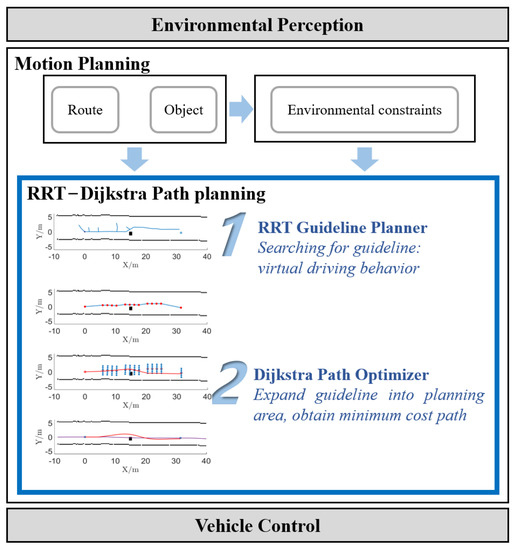
Figure 1.
Strategy architecture.
2. Problem Statement
2.1. Planning Problem Basement
The autonomous vehicle path planning problem in vast half-structured roads is formulated as a discrete optimal control problem on finding the minimum cost path, which is subject to the planning problem basement, collision avoidance constraints, and vehicle kinematic constraints.
The vehicle will travel on half-structured roads. There should always be a recommended path indicating the vehicle’s direction of movement; that is, the planning process can be applied to a Frenet coordinate system [19]. The path planning problem is finding the minimum-cost node sequence that satisfies multiple constraints connecting the start and goal points.
The path planning problem can be defined after the start point and the goal points are identified. To that end, the vehicle location in the Cartesian coordinate system [10] should be converted into in the Frenet coordinate system, and this point can be identified as the start point. The goal points are a series of points along the vertical direction of the road, defined by equations:
where is the distance between the goal point and the vehicle along axle s, is the minimum of , is the vehicle speed, is the preview time threshold, is a numerical constant, is a gain factor, and are the distance between the road reference line and the road edge at . An example of goal points is shown in Figure 2, where is a vector used to represent all possible locations, the collision-free with the minimum value can be chosen as a feasible goal point, which is in the figure.
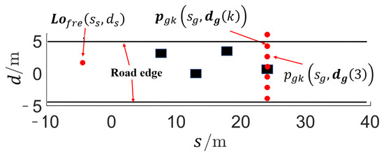
Figure 2.
Definition of .
2.2. Collision Avoidance Constraints
Collision avoidance constraints are the most complicated part of the path planning problem. In this work, an occupancy grid map is used to represent the environment, and the collision between the planned path and the obstacles can be evaluated. Here, we present two types of collision avoidance constraints: a binary occupancy grid map-based constraint and a cost occupancy map-based collision avoidance preference.
- (1)
- Binary occupancy grid map. The binary occupancy grid map is a grid map that contains information about road edges, passable areas, and obstacles to represent the environment [20]. In a binary occupancy map, each grid contains the probability of believing that there is an obstacle or not. So, the possible states of each grid are or . The grid occupancy of static obstacles can be directly projected onto the occupancy grid map by setting the corresponding grid to 1. Before projecting a dynamic obstacle onto a map, its grid occupancy should be evaluated. A simple and efficient time to collision (TTC) based approach is used to evaluate dynamic obstacles.
For a given dynamic obstacle located at on the road, its motion velocity is , velocity direction is . Its location in the Frenet coordinate system is . represents the speed of the ego vehicle at the current time . If the TTC (time to collision) time between the vehicle and the obstacle is , can be obtained through Equation (3):
where is the distance from the obstacle location point to the closest point on the obstacle to the ego vehicle. If , there will be no collision. All the dynamic obstacles on the road should be evaluated. Those are considered threatening, and those with the minimum are considered the most threatening one. represents the minimum from those obstacles with . All the locations of dynamic obstacles should be transformed into virtual locations at time and then projected onto the occupancy grid map. The virtual obstacle location of the dynamic obstacle under the Cartesian system at time can be calculated by
As shown in Figure 3b, the red square is the predicted location of virtual dynamic obstacle at time .
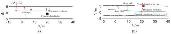
Figure 3.
An example dynamic scenario. (a) Environment model under Frenet coordinate system; (b) virtual obstacle and an example planned path at time .
After all the elements (road edges, static obstacles, dynamic obstacles, etc.) are projected onto the occupancy grid map, the environmental model is established. Similarly, the occupancy relationship brought about by the path can also be projected onto the occupancy map. The vehicle projection on the planned path at time can be obtained. The result of ( is an operator that multiplies the elements at the corresponding position in two matrices) can be used for identifying whether the vehicle projection on the planned path at time intersects the non-passable area in . If the result equals to zero, there will be no collision; otherwise, a collision occurs.
- (2)
- Cost occupancy map. The cost occupancy grid map is a grid map with different cost values, it is used for describing the cost value brought by multiple factors. An example of is shown in Figure 4 [21]. It is quite like . The difference between and is that the cost value of each grid in belongs to . The cost around the obstacle varies linearly, as does the cost of traffic rules. The calculation approach for will be introduced in detail later in this paper.
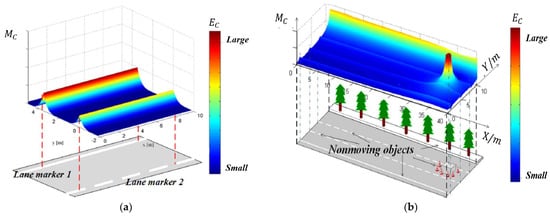 Figure 4. An example of cost occupancy map: (a) Cost of traffic rules; (b) additional cost of obstacle avoidance preference.
3. RRT-Based Guideline Planner
3.1. RRT-Based Guideline Searching Process
The guideline is generated by an RRT-based guideline planner with multiple constraints considered. This guideline is responsible for two factors: defining virtual driving behavior and reducing the wide planning area. The RRT-based planning process is shown in Algorithm 1.
| Algorithm 1. RRT searching process |
| Input: Vehicle model, environment model , start point , and goal points . |
| Output: A collision-free, dynamical driving path. |
| 1. ← InitializeTree( ); |
| 2. while ExecutionCount MaxIterationNumber |
| 3. ← SampleNewNode( ); |
| 4. if Assessment(, ) Constraints |
| 5. CONTINUE; // If is not a valid new node |
| 6. end if |
| 7. Insert to // Add into RRT-Tree if its valid |
| 8. if Distance(, ) |
| 9. BREAK; |
| 10. end if |
| 11. BackRRTPath( ); |
| 12. return ; |
Definition 1.
Function Initialize Tree ( ) is a function used for generating a basic RRT-treewith all the node being set to zero. Especially, the first node ofshould be updated to the location.
Definition 2.
Function Sample New Node ( ) is a function that generates a random new nodeinthrough a random sampling method [22].
where is a random number in . is a switching threshold that determines the convergence speed. Since this process is a rough search process, can be 0.3.
Definition 3.
Function Distance (, ) is a function that calculates the Euclidean distance between the two input points.
Definition 4.
Function Assessment (, ) is a function to assess whether the new sampled point meets the constraints or not. The point that meets all the constraints will be adapted and added to.
Definition 5.
Function BackRRTPath ( ) is a function that sortsand obtains the final feasible path.
Constraints that are mentioned in Definition 4:
- (1)
- Maximum distance constraint. The value of function Distance (, ) should meet a distance threshold . If Distance (, ) , should be resampled on the connection between and at where Distance (, ) . The RRT process in this work is a rough search process. And our initial planning area is larger than . in this work, .
- (2)
- Minimum distance constraint. The value of function Distance (, ) should be bigger than a minimum distance threshold . That is, if Distance (, ) , locates too close to the points on , should be abandoned. can be choose as .
- (3)
- Process termination constraint. This constraint is used to determine whether have reached or not. If yes, the while loop should be terminated. Basically, it is a distance defined threshold, if the distance between the new sampled node and is smaller than , reached.
- (4)
- Kinematic constraint. The yaw angle can reflect this constraint, which can be used to evaluate whether the newly sampled node can be reached by the vehicle. If the yaw angle between and (the point before ) is . The yaw angle between and is . should be less than a yaw angle threshold . .
- (5)
- Collision constraint. The paths should be collision-free. That is, the connection between and should be collision-free. should equals zero. If not, should be abandoned.
An example , and an example are shown in Figure 5.
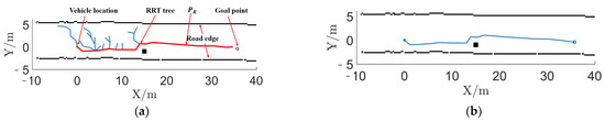
Figure 5.
An example of : (a) RRT-Tree; (b) .
3.2. Guideline Simplification
The guideline is a basic guideline, it is not smooth and even contains some unnecessary nodes. should be optimized into a guideline with fewer nodes and be smoother. An example of a simplified guideline is shown in Figure 6, it is smoother, has fewer nodes, and is collision-free, marking a smaller passable area for the vehicle to travel. For a given path sequence , a simplified guideline contains nodes can be obtained through the process represented in Algorithm 2.
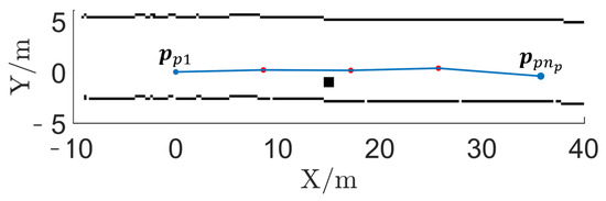
Figure 6.
An example of .
.
| Algorithm 2. Path simplification |
| Input: , |
| Output: |
| 1. ←; |
| 2. while |
| 3. ←; |
| 4. ←, ; //Update |
| 5. if ∥∥ ≥ 1 //Identify collision |
| 6. ←; //Update the current node |
| 7. else |
| 8. ←; //Update the current node |
| 9. ←; //Update simplified path |
| 10. end if |
| 11. return |
4. Dijkstra-Based Path Optimizer
4.1. Guideline Expansion
In this section, the simplified guideline will be expanded into a small planning area. In fact, the smaller passable area (or the smaller planning area) is generated at this step, obtained in Section 3 is just a guideline instead of an area. represents a smaller planning area constructed from discrete nodes. It can be obtained after is processed via a two-step expansion process, in both the s direction and the d direction (under the Frenet coordinate system). The expansion process is made up of the following two aspects.
- (1)
- Expansion along s-axle direction.
An isometric sampling strategy is introduced to expand . The nodes expect the first node (start point) and the last node (goal point) should be expanded. For a given simplified path , the expanded node sequence at the node can be calculated.
where represents the node in , is a distance threshold between adjacent nodes, represents the serial number of node , , is the number of nodes expanded at . An example of is shown by the red dots in Figure 7. Thus, the expanded node sequence along s-axle can be obtained, that is:
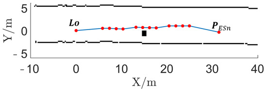
Figure 7.
An example of P_ES.
- (2)
- Expansion Along d-axle Direction.
For a given path , the nodes expect the first node (start point) and the last node (goal point) should be expanded. If contains nodes, the node sequence at node can be calculated
where the road edge at node is and , the threshold distance for sampling is , represents the number of expansions nodes along d-axle, is the sampling range threshold at node . An example of is shown by the red dots in Figure 8.
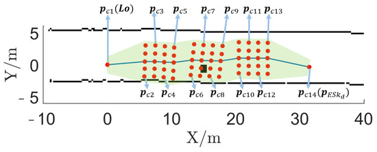
Figure 8.
An example of .
4.2. Path Candidate Generation
Nodes can make up paths, and various arrangements of nodes can create carious paths. As shown in Figure 8, represents the node cluster at one node in , and there is . For example, the second node in can be represented by . The node map can be obtained after all the connection relationships of nodes are evaluated. The connection relationship can be evaluated in two different plans: Plan A and Plan B.
- (1)
- Plan A
In each cluster , there is one node that will be selected and be added to the path candidate . An example path candidate (blue line) is shown in Figure 9.
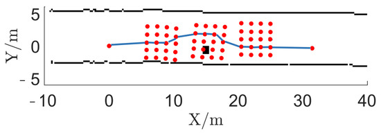
Figure 9.
An example of generated by strategy Plan A.
- (2)
- Plan B
Different from Plan A, Plan B divides node clusters based on the node . That is, the node number of each path candidate is the same as the node number in . An example path candidate (blue line) is shown in Figure 10.
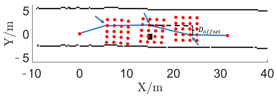
Figure 10.
An example of generated by strategy Plan B.
4.3. Path Optimization
The smaller area will be transformed into a node map , and the costs between each node in will be assessed. Therefore, the path optimization problem is modeled and transformed into a neighborhood cost assessment and discrete minimum cost sequence optimization problem. The minimum cost node sequence will be obtained via a Dijkstra-based optimizer. After the minimum cost node sequence is smoothed, the optimal path can be obtained. To that end, there are two path optimizers: Plan A and Plan B.
Every needs to be assessed. That is, every cost value between each two nodes in should be assessed. The cost node map can be obtained. So as the optimized path can be obtained through a Dijkstra process [23]. should be smoothed before it can be tracked by the vehicle. A Bezier spline curve is introduced to fit , making it smooth to meet the steering characteristics of the vehicle. An example smoothed path is shown in Figure 11.
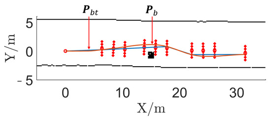
Figure 11.
An example of smoothed .
Here is an example of cost value assessment of connections between two nodes. The cost between each two nodes can be calculated.
- (1)
- is the cost of road preference. In our scenario, the autonomous vehicle is a level-four vehicle driving in specific area, there is a map marked reference path (or a reference path generated by the mission planner) with constant 50 nodes to guide the vehicle. The path planner will perform local path planning based on , thus, the vehicle should not deviate too far from . For a given connection line between two of nodes in , should be discrete into a path according to the distance threshold .
If the offset between the node can be represented by . of can be obtained
where , , and are gain coefficients, and are offset thresholds, . An example is shown in Figure 4a.
- (2)
- is the cost of vehicle dynamics.
Vehicle dynamics constraints cannot be ignored. Generally, the vehicle’s lateral acceleration can be used to calculate the cost: the smaller the cost, the smoother the path. However, the lateral acceleration cannot be directly estimated in our node map. Road curvature and relative lateral offset (under the Frenet coordinate) are chosen to calculate the cost of lateral acceleration.
where and are two gain factors, is the cost caused by the road curvature, if the cost of road offset value.
Assuming that the connection between two nodes can be divided into serval parts, the curvature (under the Cartesian coordinate system) of each part can be represented by .
can be calculated by analyzing the relative offset value between the current point and the previous node along the d-axle. The offset value at each point on the connection between two nodes can be represented by . An example between node and the th point is shown in Figure 10.
- (3)
- is the cost of other path preferences.
For a given connection between two nodes, the cost of preference should be assessed. Figure 4b shows an example cost of collision risk preference. That is, the vehicle should keep a gap from obstacles (as shown in Figure 12). The grid value in preference cost map of collision risk example can be calculated by:
where , is the map size, represent the distance from a grid to an obstacle, if the grid inside the obstacle, else the grid is outside the obstacle. represent the risks to a grid. is the maximum value of the influence range.
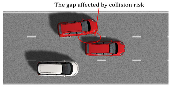
Figure 12.
An example of collision risk preference.
If represents the projection of on a binary occupancy map. can be obtained.
4.4. Speed Profile Generation
The speed profile generation is an essential part of autonomous driving systems, it generates a feasible profile based on the speed limit, and collision probability with dynamic or static obstacles, which cannot be ignored. This work focuses on the path planning process for autonomous vehicles running on half structured roads with a maximum speed limit . A simple rule-based speed profile generation approach is functional and applied to our vehicle, as shown in Figure 13. The initial target speed of the vehicle is set to . If there is no new path while the vehicle reaches the end of , the target speed is set to 0, the vehicle stops. If there is a collision on , the planned path is no longer feasible, and the target speed will be set to 0. This rule-based speed profile generation approach is also applicable to dynamic obstacles. The vehicle will stop if there are dynamic obstacles occupying the driving area, the current path has no collisions, and new paths cannot be obtained. For a dynamic obstacle following scenario, our approach theoretically allows the vehicle to follow the obstacle behind it at a distance of .
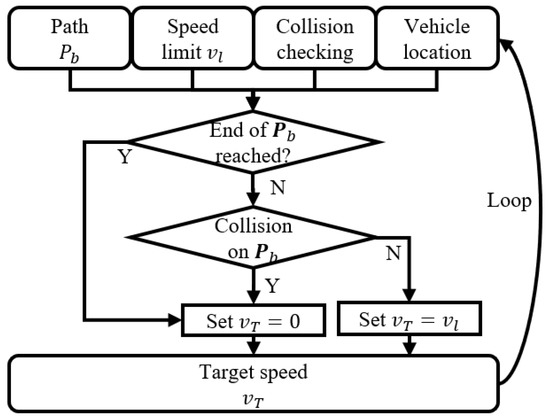
Figure 13.
Rule-based speed profile generation.
5. Simulation
5.1. Simulation Statement
Simulations are conducted with our hardware-in-loop (HIL) simulator, with the Lattice planning techniques in reference [4] as a control group. Parameters are shown in Table 1, and the simulation architecture is shown in Figure 14.

Table 1.
Simulation parameters.
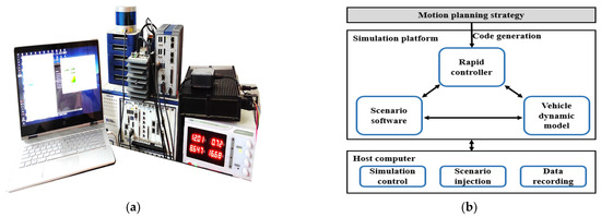
Figure 14.
Hardware-in-loop simulation platform. (a) hardware-in-loop simulation system; (b) system architecture.
5.2. Scenarios with Static Obstacles
Two scenarios with static obstacles are conducted, focusing on evaluating the performance of the planning strategy. All the scenario data is collected by an autonomous vehicle platform and reproduced on our HIL simulation platform. The ego vehicle travels at a constant speed on city roads, with obstacles in front of and around it. The simulation results are shown in Figure 15, all the paths can successfully guide vehicles to avoid obstacles. In more detail. The average results of 50 simulations under the same scenario, including Plan A, Plan B, and a classic Lattice planning strategy [4], are shown in Table 2.
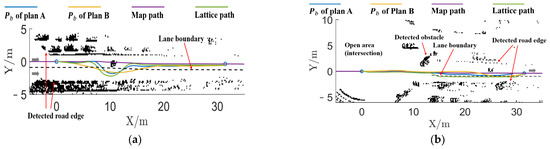
Figure 15.
Scenarios with static obstacles: (a)scenario I; (b) scenario II.
Table 2.
Comparison of two planning plans.
The path shapes of Plan A and Lattice is similar. Due to the fact that Plan A is an approximate Lattice sampling process, in which the path candidate generation and the optimal path selection is similar to those of the control group [4]. To this end, the planning accuracy can be aligned with Lattice, and the computational time has been reduced by 8 ms (22% real-time performance improvement) thanks to the introduction of a planning area reduction process in Step 1.
The path shape of Plan B is smoother and has less curvature variation than Plan A and Lattice. In particular, in Figure 15a, the path of Plan B is more in line with the human driver’s driving habits, with a gentle yaw to avoid obstacles and then a gentle return to the map path [24]. In principle, Plan B has fewer nodes than Plan A, it is more suitable for planning comfortable smooth paths in scenarios with fewer obstacles [25]. For this reason, it has the lowest planning success rate (92.5%) of the three planning strategies, but has the best real-time performance, which takes 19 ms to run once.
5.3. Scenario with Dynamic Obstacles
A scenario with dynamic obstacles is conducted to evaluate the adaptation of our strategies to dynamic scenarios. The ego vehicle runs on the road with a maximum speed of . The red point clouds represent the position of the dynamic obstacles, and the red arrows represent the motion of the dynamic obstacles. Simulation results are shown in Figure 16a.
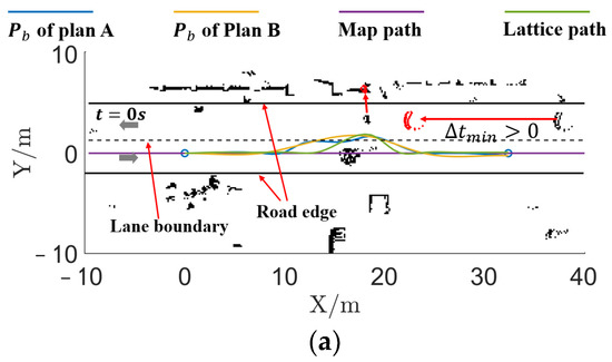
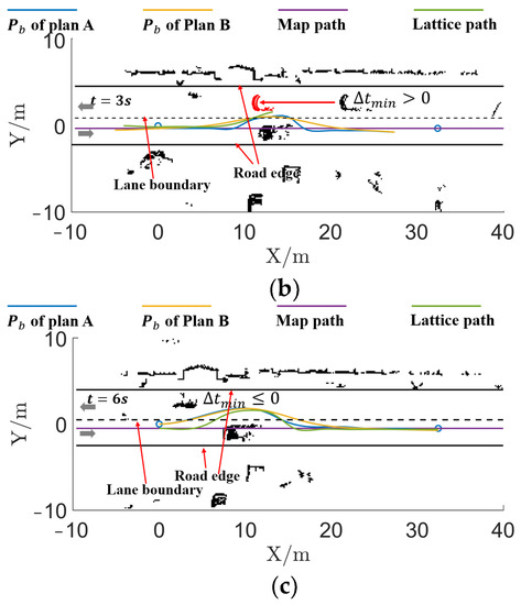
Figure 16.
Dynamic scenario. (a) Planning result at time ; (b) planning result at time ; (c) planning result at time .
The planning result at time is shown in Figure 16a. The point clouds of dynamic obstacles are projected onto the map, where the planning task for a dynamic scenario is transformed into the planning task for a static scenario. Similar to the results in Section 5.2., the planning results for Plan A and Lattice [4] are similar, and the result for Plan B is smoother and more easily executed by the vehicle [26].
The planning result at time is shown in Figure 16b, where it is interesting to note that the Lattice strategy did not yield any feasible paths, but Plan A and Plan B are still functional. Yet, for the Lattice planner, there is no feasible collision-free path for the vehicle to travel, as the predicted point clouds of the dynamic obstacles occupied all feasible areas, and as the Lattice planner is not flexible enough [25]. The target speed is set to zero , the vehicle stops. For Plan A and Plan B, thanks to the search strategy in Step 1, the planning area reduction process, which brings a stochastic process with more flexibility, where the RRT process in Step 1 refreshes until the boundary constraints are reached if there is no feasible path.
The planning result at time is shown in Figure 16c. The dynamic obstacle has passed the ego vehicle and been assessed as no threat, where . The planning task for a dynamic scenario regress into normal planning task for a static scenario.
6. Conclusions
This paper presented a path planning strategy for autonomous vehicles traveling on half-structured roads. The challenge of path planning was split into two issues. (1) An RRT-based planner, which turned the large-scale planning problem into a small-scale planning problem, lowered the planning area. Due to its random sampling feature, the RRT approach increased process flexibility. (2) By turning the smaller planning area into a discrete multi-source cost optimization problem, the planning problem was solved. Two strategies were established to address the issue: with Plan A it was more flexible; Plan B was more efficient. (3) Simulation results proved that our proposal was efficient and effective in both static and dynamic scenarios. Although the planned path was not optimal, it consumed less computing power (20% real-time performance improvement) and there was no significant loss of accuracy (compared with a Lattice planner).
In our future work, numerical optimization methods incorporating additional vehicle kinematic constraints, dynamic constraints, and other constraints, will be applied to this two-step strategy to enhance search completeness. Instead of obtaining discrete suboptimal paths, optimal paths could be obtained.
Author Contributions
Conceptualization, R.C., J.H. and W.X.; methodology, R.C. and J.H.; software, R.C. and W.X.; validation R.C.; resources, J.H.; data curation, W.X.; writing R.C.; funding acquisition R.C. and J.H. All authors have read and agreed to the published version of the manuscript.
Funding
All the authors would like to express our gratitude to all those who helped us improve this work. And the authors are grateful for the support provided by “Hubei Provincial Department of Science and Technology (2019AEA169)”, “Hubei Provincial Department of Science and Technology (2020AAA001)” and “The Fundamental Research Funds for the Central Universities (2020-YB-020)”.
Institutional Review Board Statement
Not applicable.
Informed Consent Statement
Not applicable.
Data Availability Statement
The data used to support the findings of this study are available from the corresponding author upon request.
Acknowledgments
The authors wish to thank Kai Cao from Dongfeng Usharing Technology Co., Ltd. (Wuhan, China), for valuable discussion and the constructive comments on the experiments.
Conflicts of Interest
The authors declare that they have no known competing financial interest or personal relationships that could have appeared to influence the work reported in this paper.
References
- Guo, J.; Sun, M.; Wang, T.; Lu, L. Transportation Development and Congestion Mitigation Measures of Beijing, China. Mitig. Adapt. Strateg. Glob. Chang. 2015, 20, 651–663. [Google Scholar] [CrossRef]
- Jiang, Y.; Jin, X.; Xiong, Y.; Liu, Z. A Dynamic Motion Planning Framework for Autonomous Driving in Urban Environments. In Proceedings of the Chinese Control Conf. CCC, Shenyang, China, 27–30 July 2020; pp. 5429–5435. [Google Scholar] [CrossRef]
- Sharma, O.; Sahoo, N.C.; Puhan, N.B. Recent Advances in Motion and Behavior Planning Techniques for Software Architecture of Autonomous Vehicles: A State-of-the-Art Survey. Eng. Appl. Artif. Intell. 2021, 101, 104211. [Google Scholar] [CrossRef]
- Hu, J.; Chen, R.; Xu, W.; Lu, R. An Event-Triggered Real-Time Motion Planning Strategy for Autonomous Vehicles. Proc. Inst. Mech. Eng. Part C J. Mech. Eng. Sci. 2022, 236, 10332–10348. [Google Scholar] [CrossRef]
- Okumura, B.; James, M.R.; Kanzawa, Y.; Derry, M.; Sakai, K.; Nishi, T.; Prokhorov, D. Challenges in Perception and Decision Making for Intelligent Automotive Vehicles: A Case Study. IEEE Trans. Intell. Veh. 2016, 1, 20–32. [Google Scholar] [CrossRef]
- Noh, S.; An, K. Decision-Making Framework for Automated Driving in Highway Environments. IEEE Trans. Intell. Transp. Syst. 2018, 19, 58–71. [Google Scholar] [CrossRef]
- Dolgov, D.; Thrun, S.; Montemerlo, M.; Diebel, J. Path Planning for Autonomous Vehicles in Unknown Semi-Structured Environments. Int. J. Rob. Res. 2010, 29, 485–501. [Google Scholar] [CrossRef]
- Fan, H.; Zhu, F.; Liu, C.; Zhang, L.; Zhuang, L.; Li, D.; Zhu, W.; Hu, J.; Li, H.; Kong, Q. Baidu Apollo EM Motion Planner. arXiv 2018, arXiv:1807.08048. [Google Scholar]
- Zhang, S.; Deng, G.; Yang, E.; Ou, J. Optimal Vehicle Lane Change Trajectory Planning in Multi-Vehicle Traffic Environments. Appl. Sci. 2022, 12, 9662. [Google Scholar] [CrossRef]
- Eskandarian, A. Handbook of Intelligent Vehicles; Springer: Cham, Switzerland, 2012; pp. 1–1599. [Google Scholar] [CrossRef]
- Nazarahari, M.; Khanmirza, E.; Doostie, S. Multi-Objective Multi-Robot Path Planning in Continuous Environment Using an Enhanced Genetic Algorithm. Expert Syst. Appl. 2019, 115, 106–120. [Google Scholar] [CrossRef]
- Wang, Z.; Li, G.; Jiang, H.; Chen, Q.; Zhang, H. Collision-Free Navigation of Autonomous Vehicles Using Convex Quadratic Programming-Based Model Predictive Control. IEEE/ASME Trans. Mechatron. 2018, 23, 1103–1113. [Google Scholar] [CrossRef]
- Van Dang, C.; Ahn, H.; Lee, D.S.; Lee, S.C. Improved Analytic Expansions in Hybrid A-Star Path Planning for Non-Holonomic Robots. Appl. Sci. 2022, 12, 5999. [Google Scholar] [CrossRef]
- Li, A.; Niu, C.; Li, S.; Huang, X.; Xu, C.; Liu, G. Research on Intelligent Vehicle Trajectory Planning and Control Based on an Improved Terminal Sliding Mode. Appl. Sci. 2022, 12, 2446. [Google Scholar] [CrossRef]
- Collin, A.; Bilka, A.; Pendleton, S.; Tebbens, R.D. Safety of the Intended Driving Behavior Using Rulebooks. In Proceedings of the IEEE Intelligent Vehicles Symposium IV, Las Vegas, NV, USA, 19 October–12 November 2020; pp. 136–143. [Google Scholar] [CrossRef]
- Li, B.; Liu, S.; Tang, J.; Gaudiot, J.-L.; Zhang, L.; Kong, Q. Autonomous Last-Mile Delivery Vehicles in Complex Traffic Environments. Computer 2020, 53, 26–35. [Google Scholar] [CrossRef]
- Mozaffari, S.; Al-Jarrah, O.Y.; Dianati, M.; Jennings, P.; Mouzakitis, A. Deep Learning-Based Vehicle Behavior Prediction for Autonomous Driving Applications: A Review. IEEE Trans. Intell. Transp. Syst. 2022, 23, 33–47. [Google Scholar] [CrossRef]
- Hou, Z.; Liu, H.; Zhang, Y. Zero-Day Vulnerability Inspired Hazard Assessment for Autonomous Driving Vehicles. In Proceedings of the IEEE 19th International Conference on Communication Technology (ICCT), Xi’an, China, 16–19 October 2019; pp. 1348–1354. [Google Scholar] [CrossRef]
- Werling, M.; Ziegler, J.; Kammel, S.; Thrun, S. Optimal Trajectory Generation for Dynamic Street Scenarios in a Frenét Frame. In Proceedings of the IEEE International Conference on Robotics and Automation, Anchirage, AK, USA, 3–7 May 2010; pp. 987–993. [Google Scholar] [CrossRef]
- Huang, Y.; Ding, H.; Zhang, Y.; Wang, H.; Cao, D.; Xu, N.; Hu, C. A Motion Planning and Tracking Framework for Autonomous Vehicles Based on Artificial Potential Field Elaborated Resistance Network Approach. IEEE Trans. Ind. Electron. 2020, 67, 1376–1386. [Google Scholar] [CrossRef]
- Wang, J.; Wu, J.; Zheng, X.; Ni, D.; Li, K. Driving Safety Field Theory Modeling and Its Application in Pre-Collision Warning System. Transp. Res. Part C Emerg. Technol. 2016, 72, 306–324. [Google Scholar] [CrossRef]
- Karaman, S.; Walter, M.R.; Perez, A.; Frazzoli, E.; Teller, S. Anytime Motion Planning Using the RRT. In Proceedings of the IEEE International Conference on Robotics and Automation, Shanghai, China, 9–13 May 2011; pp. 1478–1483. [Google Scholar] [CrossRef]
- Zhu, Z.; Li, L.; Wu, W.; Jiao, Y. Application of Improved Dijkstra Algorithm in Intelligent Ship Path Planning. In Proceedings of the 33rd Chinese Control and Decision Conference, Kunming, China, 22–24 May 2021; pp. 4926–4931. [Google Scholar] [CrossRef]
- Kim, J.; Kum, D. Collision Risk Assessment Algorithm via Lane-Based Probabilistic Motion Prediction of Surrounding Vehicles. IEEE Trans. Intell. Transp. Syst. 2018, 19, 2965–2976. [Google Scholar] [CrossRef]
- Claussmann, L.; Revilloud, M.; Gruyer, D.; Glaser, S. A Review of Motion Planning for Highway Autonomous Driving. IEEE Trans. Intell. Transp. Syst. 2015, 57, 1826–1848. [Google Scholar] [CrossRef]
- Li, B.; Ouyang, Y.; Li, L.; Zhang, Y. Autonomous Driving on Curvy Roads Without Reliance on Frenet Frame: A Cartesian-Based Trajectory Planning Method. IEEE Trans. Intell. Transp. Syst. 2022, 23, 15729–15741. [Google Scholar] [CrossRef]


Publisher’s Note: MDPI stays neutral with regard to jurisdictional claims in published maps and institutional affiliations. |
© 2022 by the authors. Licensee MDPI, Basel, Switzerland. This article is an open access article distributed under the terms and conditions of the Creative Commons Attribution (CC BY) license (https://creativecommons.org/licenses/by/4.0/).