Simulation on Unsteady Crosswind Forces of a Moving Train in a Three-Dimensional Stochastic Wind Field

Abstract

Unsteady aerodynamic forces are significantly critical to the safety and stability of trains traveling in high winds. This paper describes a study into unsteady crosswind forces of a moving train subjected to a three-dimensional stochastic wind field with longitudinal, lateral, and vertical turbulences. Initially, a three-dimensional computational fluid dynamic (CFD) model is established to calculate the aerodynamic coefficient of a moving train, and then the wind velocity time histories at the position of the train are generated. Finally, the quasi-steady theory and weighting function method are used to model the unsteady crosswind forces of a moving train in a three-dimensional turbulence field. The results demonstrate that a generalized sine form is useful for predicting the aerodynamic coefficient that varies with the resultant wind yaw angle, and an adequate modeling of unsteady crosswind forces with complete wind turbulences can produce a greater force fluctuation and peak. Particularly when the flow direction of crosswind deviates from 90°, consideration of only a portion of the turbulence components may underestimate the dynamic response of trains.

1. Introduction

It is becoming increasingly common for trains to travel at faster speeds and lighter weights, which increases the safety risk under crosswinds. Several incidents of train derailment or overturning caused by strong winds have been reported in recent decades in China, Japan, Belgium, and Switzerland [1,2,3]. The overturning and stability problems of railway vehicles exposed to crosswinds also have attracted a lot of attention over the years [4,5,6,7,8,9,10,11,12]. Currently, the overturning assessments of trains are frequently carried out in the time domain using dynamic multi-body simulation, which requires first and foremost the precise calculation of stochastic aerodynamic forces to accurately quantify the dynamic response of trains.

One of the essential works is to determine the aerodynamic force coefficients of trains in the simulation of unsteady crosswind forces, usually conducted by the full-scale experiment, scaled wind tunnel test, or numerical calculation, and many pieces of research on this aspect have been reported [13,14,15,16,17]. It is worth noting that a static train model is typically used to equivalently simulate the aerodynamic coefficients of moving trains by means of the resultant wind velocity and yaw angle, which cannot accurately reproduce the flow characteristics between the moving train and the infrastructure. Thus, recent works have developed several moving model systems associated with the train traveling on bridges in wind tunnels [18,19,20,21]. With the rapid development in computing power, the numerical technique is increasingly being used in civil engineering to address some aerodynamic problems associated with high-rise buildings, long-span bridges [22,23,24], where some flow details of structures can be captured and reproduced graphically. Also, the CFD method is possible to be applied to simulate the flow features of a high-speed train in crosswinds [25,26] by using the moving mesh algorithm, including sliding mesh [27,28], dynamic mesh [29,30], and overset mesh [15,31], is easily applied to simulate the flow field around a high-speed train. There are also some simplified expressions proposed to describe the effect of the resultant yaw angle on the aerodynamic force coefficients of moving trains [6,32,33,34].

The stochastic simulation of fluctuating wind speed time histories relative to a moving train is another fundamental work for calculating unsteady forces. Cooper [35] initially proposed a stochastic wind model with respect to a moving vehicle in light of the von-Karman spectrum based on Taylor’s frozen turbulence hypothesis. On the basis of work by Cooper, Baker [34] developed a simple and robust approach for calculating the fluctuating wind speed time series of a moving train and demonstrated how wind turbulence in crosswinds produces fluctuating forces through the use of weighting function from experimental data of aerodynamic admittance. Yu et al. [36] also generated stochastic force time histories with longitudinal and lateral turbulences using the wind spectrum developed by Cooper to investigate the dynamic behavior of a China railway high-speed train in windy environments. Wu et al. [37] used a numerical approach to derive the wind spectrum and correlation function for vehicles traveling through a cross wind field from the Kaimal spectrum, and furthermore, Li et al. [3], Yan et al. [38], and Hu et al. [39] provided more general and appropriate expressions for the wind spectrum of a moving vehicle for various turbulent wind models. Interpolation from fixed points on the traveling line, on the other hand, is an alternative method for calculating the fluctuating wind speeds of a moving train. With the use of interpolating results, Li et al. [40] set up an approximation formula for predicting the wind loads acting on vehicles traveling at longitudinal and vertical wind turbulences in the wind-vehicle-bridge system, and Xu and Ding [4] further considered the effect of aerodynamic admittance functions on unsteady aerodynamic forces. Cheli et al. [41] also reproduced the time-space distribution of the turbulent wind and introduced a stochastic methodology of aerodynamic loads on trains to evaluate the crosswind stability of trains by means of the characteristic wind curves.

However, it should be noted that the complete turbulence field is not considered in the simulation of unsteady crosswind forces on trains in the aforementioned studies, which may result in an underestimation of the force fluctuation and peak caused by the wind turbulence. As a matter of fact, a train traveling through crosswinds will experience three-dimensional stochastic wind turbulence with longitudinal, lateral, and vertical components. Yu et al. [36] pointed out that lateral turbulence cannot be ignored in the analysis of train operational safety if cross wind is not normal to the car body. As a result, the chief work of this study is to propose a formula for predicting unsteady crosswind forces on a moving train in the presence of a complete turbulence field, which is a further development and improvement for previous investigations by Baker [34], Yu et al. [36] and Li et al. [40]. Specifically, it establishes a prediction model for train force coefficients using CFD simulated data and details how wind turbulence with longitudinal, lateral, and vertical components at various crosswind directions produce fluctuating forces of a moving train through a simple mathematical derivation. The findings of this study are useful for precisely calculating dynamic responses and accurately assessing the running safety of trains caused by crosswinds in future investigations.

This paper is organized as follows. In Section 2, the computational algorithm and brief details of the CFD model are presented and the numerical accuracy is validated by a scaled wind test. Section 3 describes the flow characteristics of a moving train traveling on a viaduct and proposes a model for predicting the aerodynamic coefficient varying with the resultant yaw angle. Section 4 introduces an interpolating method and a moving point approach for generating the fluctuating wind velocity time series at the position of the train. In Section 5, the calculation formula of unsteady crosswind forces on a moving train that takes into account the complete turbulence field is developed, and the effects of the weighting function and crosswind direction on unsteady forces are explored using numerical examples. Finally, some broad conclusions are drawn and further works are discussed in Section 6.

2. CFD Numerical Model

2.1. Governing Equations and Turbulence Model

The crosswind flow field around a moving train performs three-dimensional complicated and unsteady features, which usually can be described by the large eddy simulation (LES), detached eddy simulation (DES) and Reynolds-Average Navier-Stokes (RANS) numerical methods. However, the LES and DES are very computationally intensive for the work presented in this research associated with a moving train due to their requirements for the high-quality and high-density grid in the calculation. In fact, the RANS turbulence model is the dominant approach in simulating the flow evolution characteristics of the railway rolling stock under cross winds, owing to its efficiency and accuracy. In order to correctly capture the flow structure on the train surface, the SST (shear stress transport) k-ω turbulence model based on RANS two equations was adopted in this study, and it is assumed that the flow is incompressible. Thus, the continuity and momentum conservation equations in tensor form are respectively expressed as follows:

$$\frac{\partial }{\partial x_i}\left(\rho u_i\right)=0$$

(1)

$$\frac{\partial {\left(\rho u\right)}_i}{\partial t}+\frac{\partial }{\partial x_j}\left(\rho u_i{u}_j\right)=-\frac{\partial p}{\partial x_i}+\frac{\partial }{\partial x_i}\left(\mu \frac{\partial u_i}{\partial x_j}-\rho \overline{u_i^{\prime }{u}_j^{\prime }}\right)+F_i$$

(2)

where ρ is the air density; u and u′ are the mean and fluctuating speed components, respectively; p is the air pressure; F is the force of unit mass; the subscripts i, j = 1, 2, 3 present the x, y, z directions, respectively.

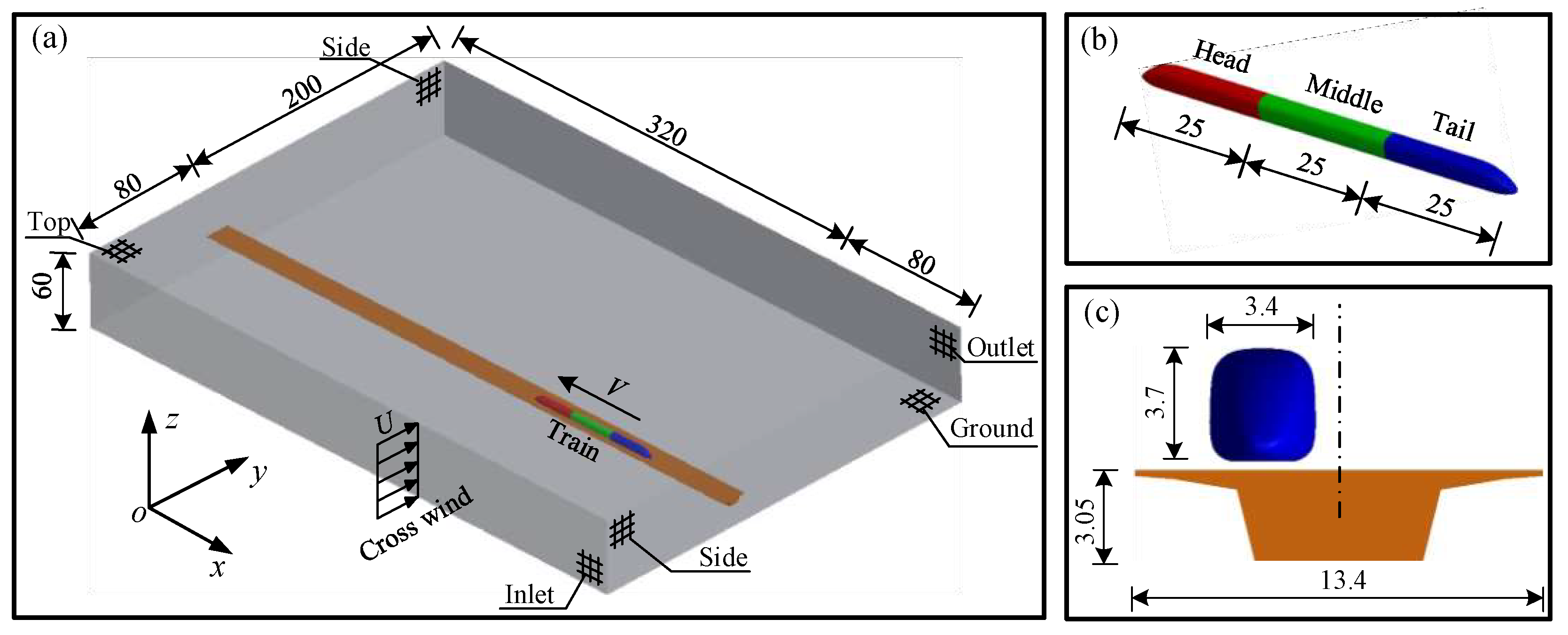
2.2. Model Descriptions

The CFD simulation is conducted using a full-scale dimension, and the typical China railway high-speed train running on a viaduct is used as the geometric model. In order to possibly minimize the boundary effect and fully reproduce the wake flow, a fluid domain with a suitable size has to be chosen first. Referring to the related investigations conducted by Zhai et al. [5] and Yao et al. [15], the flow domain is set as a parallelepiped in 400 × 280 × 60 m key dimensions for the simulation of a moving train in crosswinds, where the bridge is 80 m from the upstream and the train runs for 240 m on the bridge, and the size of the flow domain is also calibrated by several trial calculations, shown in Figure 1a. A uniform inlet velocity boundary condition with a mean velocity U and 5% low turbulence intensity is applied on the inlet of the fluid zone, and the outlet is a zero-gauge pressure outlet boundary. The top and side surfaces of the computational domain are defined as the no-slip wall, and the boundary effect on the surfaces of train and bridge and the ground is performed by the no-slip wall with a standard wall function.

The complete CRH train in 200 m length is out of available computing resources. Thus, the total train length in the simulation is limited to 75 m assembly consisting of a head car, a middle car, and a tail car, and the full-scale width and height dimensions of a train are 3.4 and 3.7 m, respectively, as illustrated in Figure 1b,c. Besides, the train geometry in the calculation is further simplified to smooth curved surfaces without regard to the effects of wheelsets, mirrors, windshield wipers and other attached parts. The bridge geometry with a width of 13.4 m and height of 3.05 m is originated from the 32 m-span simply supported box beam widely used in China high-speed railways, and the attached structures on the bridge, such as railings, tracks and contact networks are also neglected.

The hexahedral-dominated mesh is utilized to discretize the flow domain in this study. A proper resolution is required close to the train surface to correctly simulate the flow structure. Therefore, a finer mesh density adopting a minimum of 5 mm size is generated in the region near the train and bridge, and then the size is gradually running to 0.2 m in the coarse region, as shown in Figure 2a. It is noted that the boundary layer mesh of a 6 mm total thickness is arranged on the train and bridge surfaces to capture the wall flow accurately, in which the initial layer thickness is created to 0.6 mm and then it expands to 5th layers at a ratio of 1.2, as shown in Figure 2c. The corresponding dimensionless wall distance y⁺ is close to 1, and finally, the total mesh number in this numerical model is about 15 million.

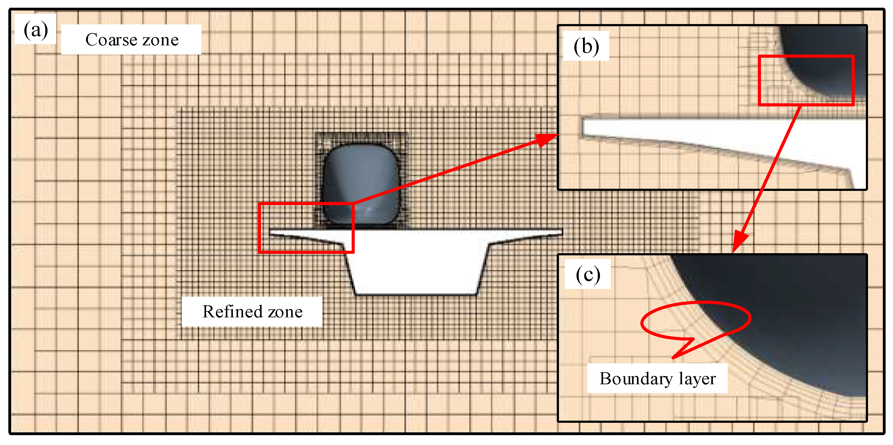
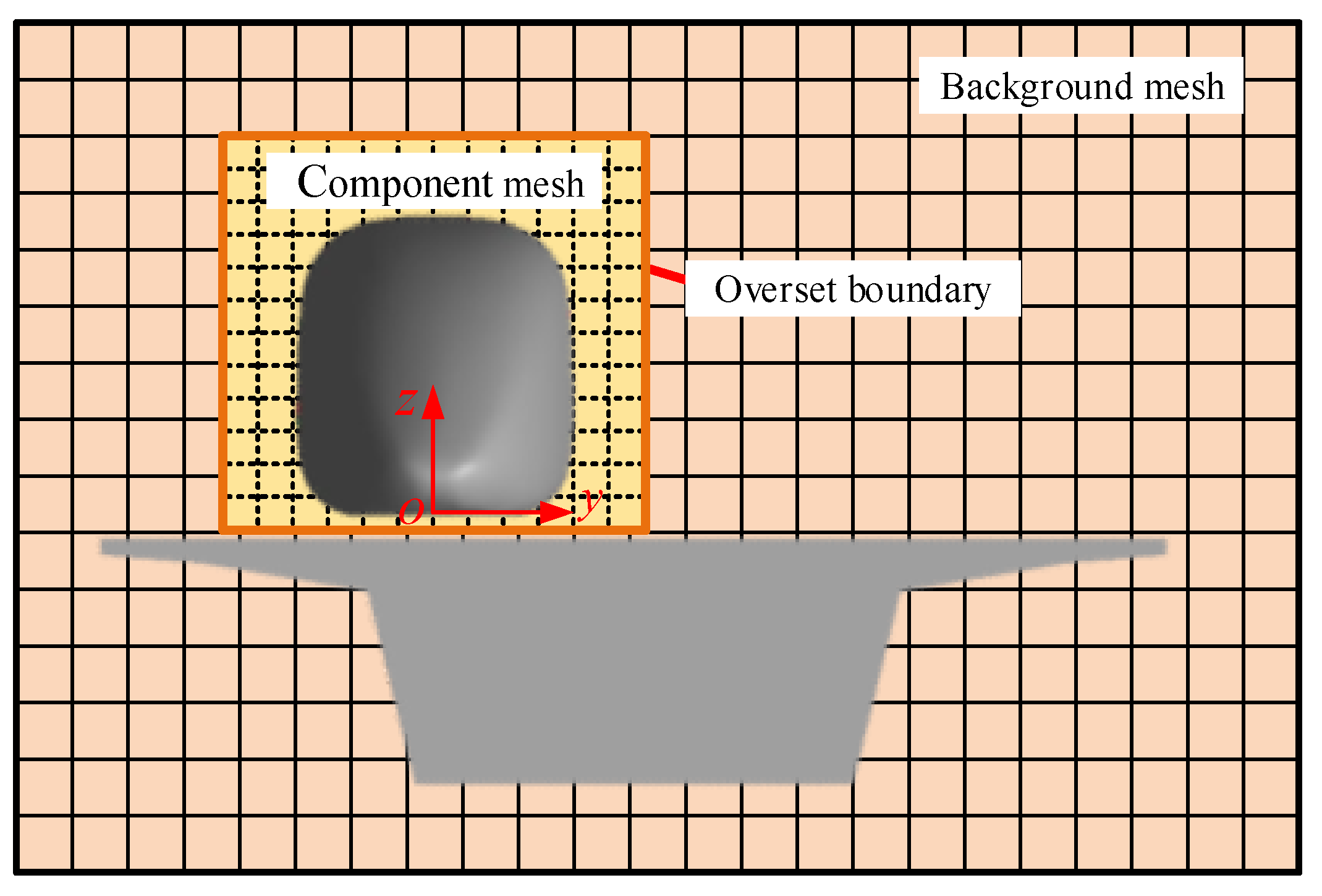
2.3. Overset Mesh

When the effect of moving trains must be concerned, the sliding and remeshing methods are frequently used in related research of numerical simulations [27,28,29,30,31]. However, a novel overset mesh technique, also called ‘Chimera’ or overlapping methodology, is applied in this study for its advantages in problems dealing with multiple or moving parts, where the individual mesh of moving parts can be created independently with fewer constraints to avoid that the parts have to fit together conformally or along non-conformal interfaces, which is useful for some complex and irregular moving bodies in the flow. In the case of overset meshes, the flow domain consists of two parts—a static background zone and one or more dynamic component zones involving moving parts. In the moving train case described in this study, the background zone that makes up the background mesh of the computational domain includes the bridge model and outer flow boundary face, and the train model is subjected to a component zone with a rectangular volume of air around it, as seen in Figure 3. The outer boundary of the component zone, an overlapping interface between two cell zones, is specified as the overset boundary condition to exchange the flow field information between two cell zones. The moving train effect is performed by means of a moving coordinate system established on the train bottom in the component zone. When the time-step of a train movement is given, the component zone starts to move in the flow domain and the overset boundary is also automatically updated.

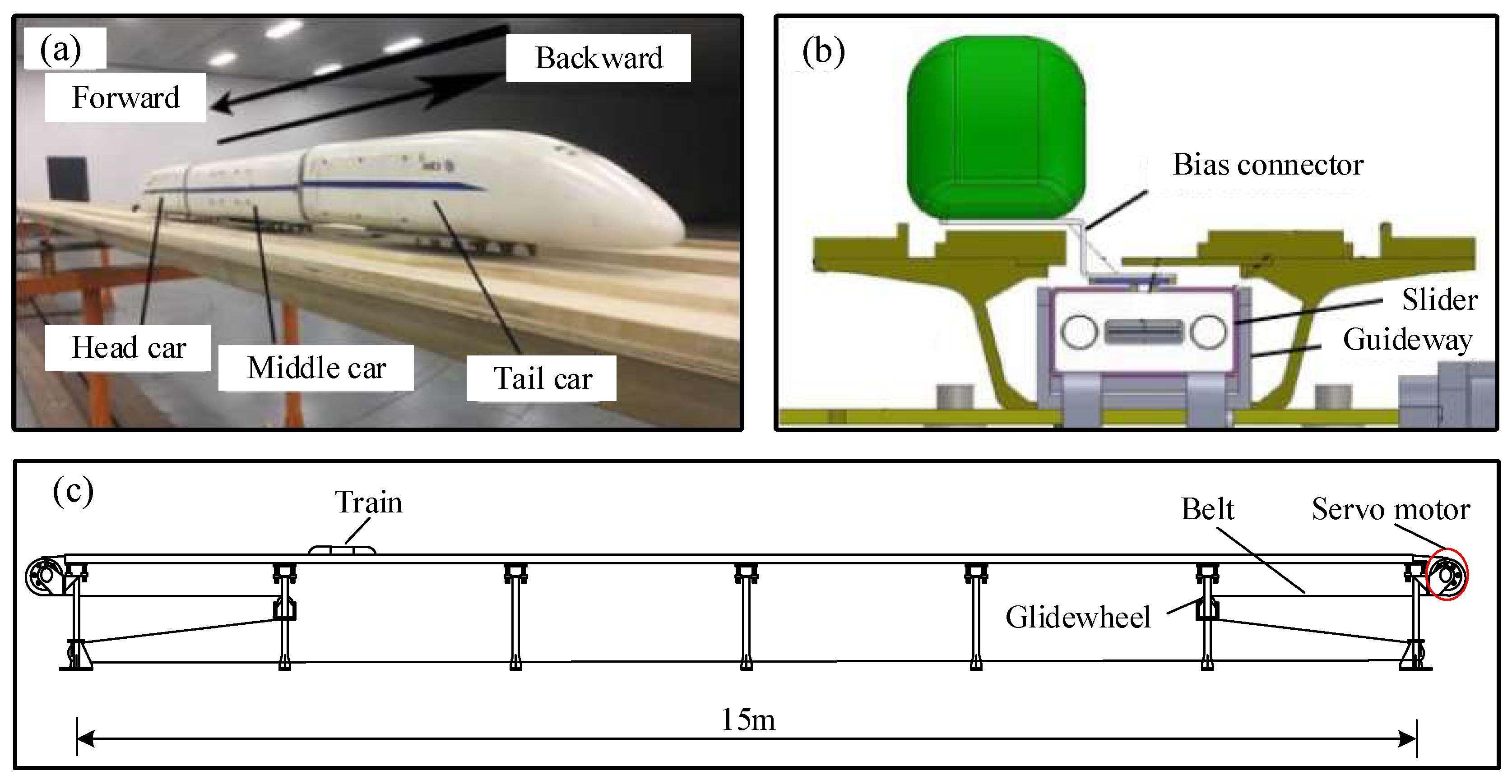
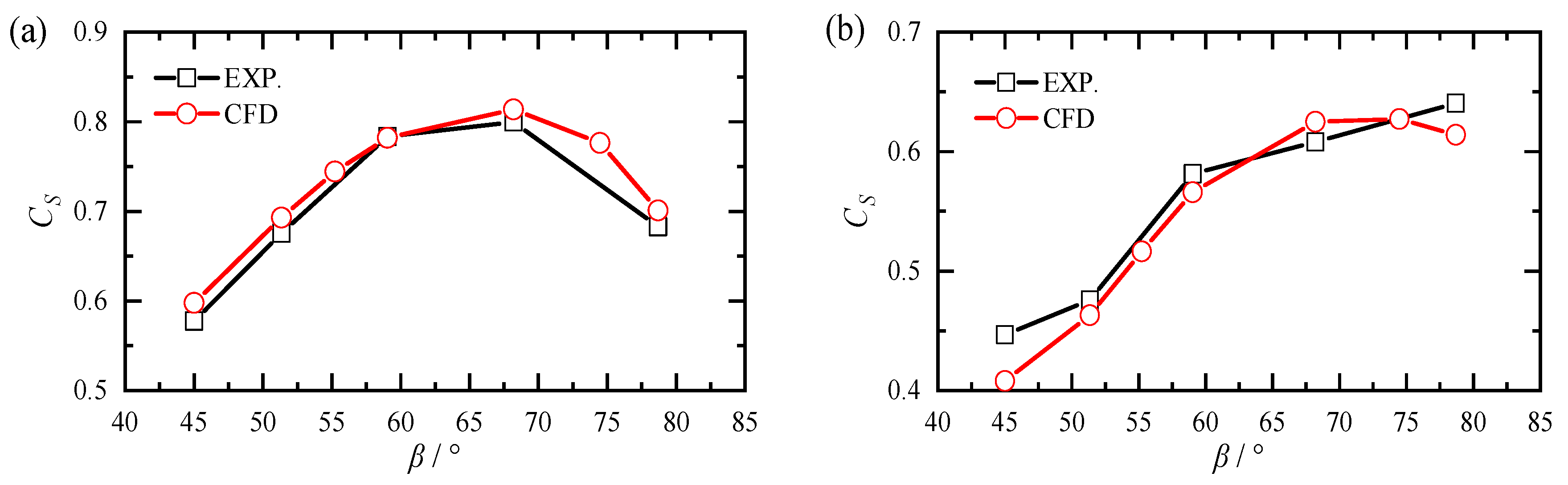
2.4. CFD Validation

In order to validate the accuracy and reliability of CFD simulation, the train aerodynamic coefficients are compared with the results of a 1/30 scaled moving wind tunnel model carried out by Shai [42] and Li et al. [16] on account of the same shape of train and bridge model in the simulation. The scaled model experiment was conducted in the XNJD-3 wind tunnel with dimensions of 36.0 × 22.5 × 4.5 m, and the entire test system is composed of a train model, bridge model and driving system. Figure 4 displays the arrangements and details associated with the wind tunnel test, where the train consisting of three cars (head, middle and tail) is connected to the moving slider on the guideway by the bias connector to run on a bridge with the use of the motor driving system, and two wireless force transducers are placed inside the head and middle cars to collect the aerodynamic force time history of the train. In the experiment, the train steadily travels 15 m on the bridge at a constant speed ranging from 0 to 8 m/s, and the wind speed varies from 0 to 10 m/s. All test settings in the wind tunnel are identically applied in the validation.

A great number of related works have demonstrated that the aerodynamic coefficient of a moving train can be determined by the resultant wind speed and wind yaw angle. As seen in Figure 5, through the geometric relation, the resultant wind speed V_R and wind yaw angle β on a moving train are able to be given by the speed vectors:

$$V_R=\sqrt{{\left(V+U\cos \alpha \right)}^2+{\left(U\sin \alpha \right)}^2}$$

(3)

$$\beta =\arctan \frac{U\sin \alpha }{V+U\cos \alpha }$$

(4)

where U and V are the wind speed and train speed, respectively; α is the angle between the cross wind and traveling line. Thus, the key aerodynamic coefficients of a moving train associated with crosswind stability can be defined as follows:

$$C_S=F_y/\left(\frac{1}{2}\rho A_y{V}_R^2\right)$$

(5)

$$C_L=F_z/\left(\frac{1}{2}\rho A_z{V}_R^2\right)$$

(6)

$$C_R=M_x/\left(\frac{1}{2}\rho A_{z}h{V}_R^2\right)$$

(7)

where C_S, C_L and C_R are the train aerodynamic coefficients of the side force F_y, lift force F_z and rolling moment M_x, respectively; ρ is the air density; A_y and A_z are the train area in the y and z direction, respectively; h is the train height.

Figure 6 shows the comparison results of the train’s aerodynamic coefficients in the simulation and test. It should be noted that only side force results are given for the consideration that the lift force can be easily affected by the turbulence characteristics and complex structures underneath the train, and the rolling moment is usually determined by the side force. It can be seen from Figure 6 that the experimental and numerical results of the head car in the various yaw angles are in a good level of agreement, while several individual data in the middle car between the numerical calculation and wind tunnel test are slightly different. As a matter of fact, it cannot be expected to obtain exactly identical agreement in the comparison results owing to the turbulent flow. The maximum error between the simulation and test is about 7%, usually which is acceptable in CFD calculation. Consequently, the comparison results indicate the numerical model in this study can sufficiently fulfill the simulation of a moving train in a crosswind.

3. Prediction Model of Aerodynamic Coefficients

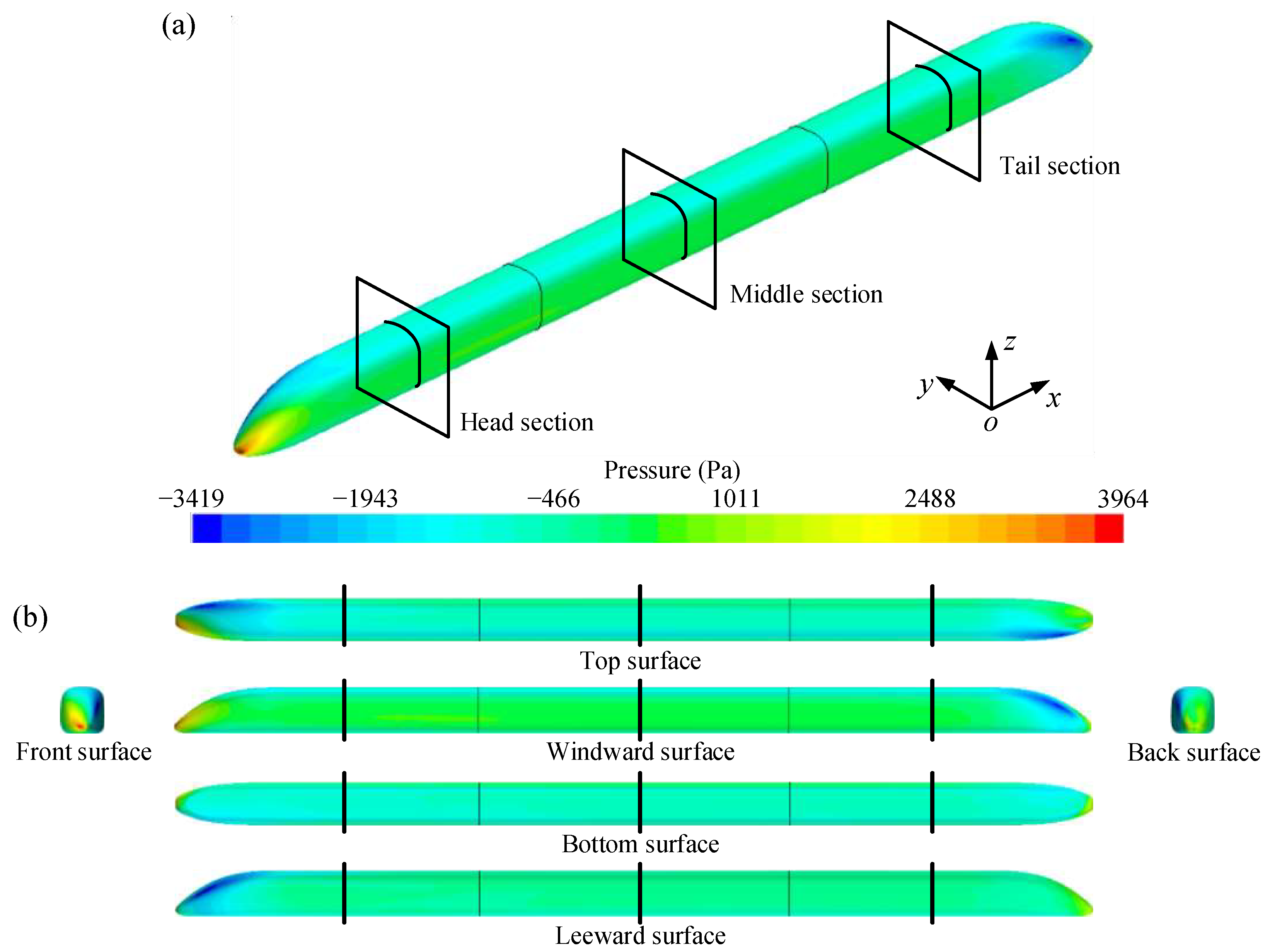
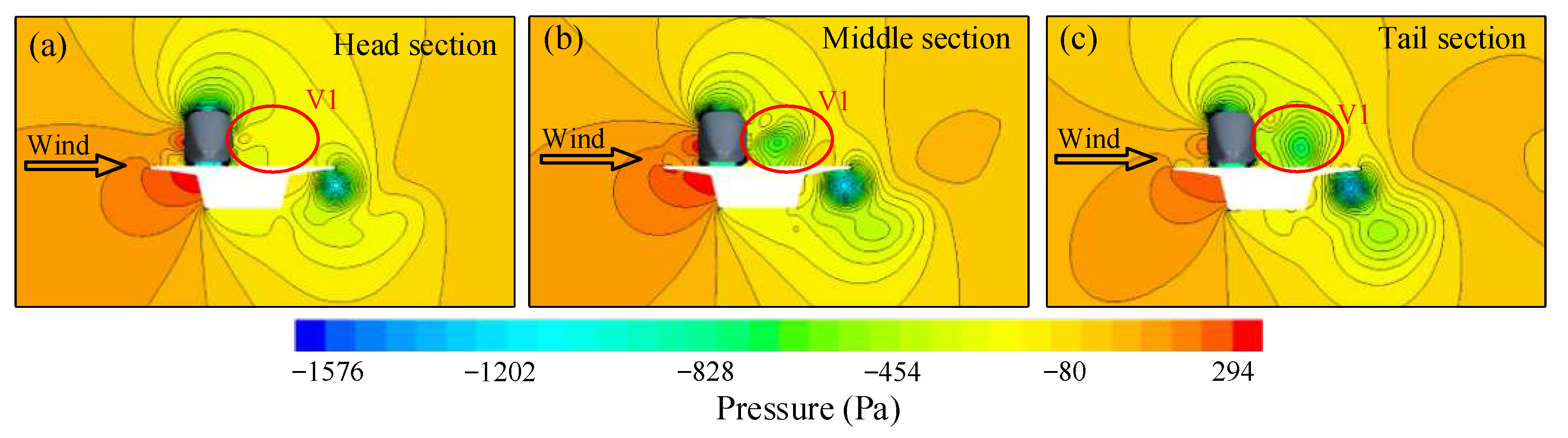
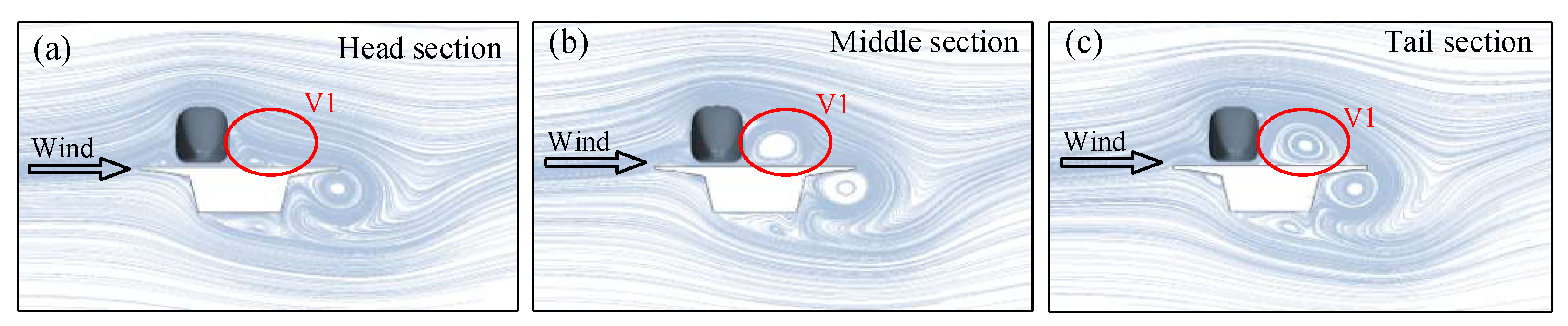
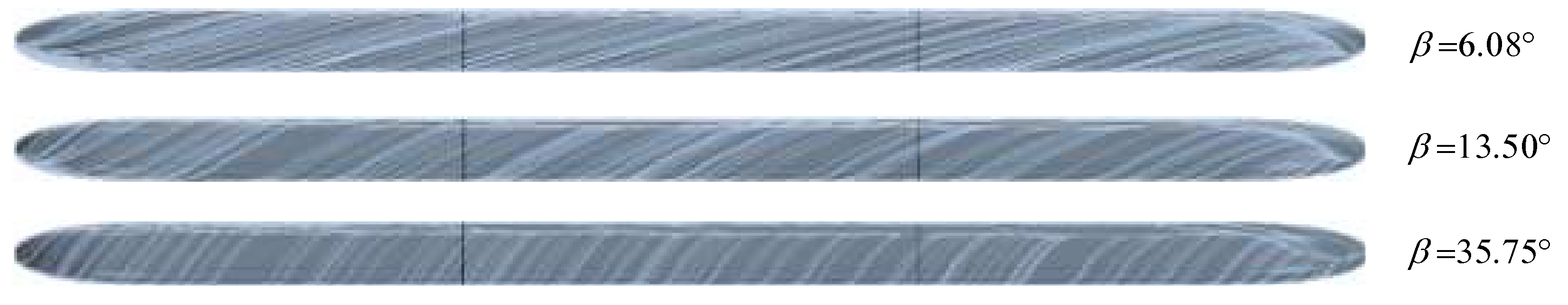
3.1. Flow Characteristics

The surface pressure distribution of a moving train exposed to cross wind is demonstrated in Figure 7. It can be clearly observed that an obvious positive pressure is found on the nose region of the head car as a result of the compression effect of a running train on air ahead. However, the pressure is not symmetrically distributed but concentrated in the windward resulting from the impacts of crosswind. The negative pressure peak appears on the leeward roof corner of the head car and on the windward roof corner of the tail car, perhaps indicating there is some separate flow in this region. Furthermore, it can be seen from Figure 7b that the positive pressure is mostly distributed on the windward surface, while the negative pressure is focused on the other train surfaces, probably leading to the major side force of the train.

In order to explore the spatial flow characteristics of a moving train in a crosswind, the pressure and streamline at three typical sections on the x-axis are reported in Figure 8 and Figure 9, respectively. As can be seen, the flow on the windward at different sections is similar but differs on the leeward. To be specific, the wake vortex (V1) of the train on the leeward gradually increases from the head car to the tail car. In fact, when the train is traveling at high speed, the airflow around the train also will move to result in the train-induced wind due to the viscous of fluids. Thus, the flow field of the train is characterized by three-dimensional structures under the combination of train-induced wind and crosswind. The wind tunnel work of an idealized train model by Copley [43] also revealed that at the presence of an opening crosswind condition, the flow pattern of a moving train on the leeward is a variety of three-dimensional inclined wake vortices along the length of the car body. The simulated work of Yao et al. [15] further indicated that the aerodynamic interaction resulting from a moving train and crosswind can produce the complex three-dimensional flow on the train leeward. In terms of Equations (3) and (4), the aerodynamic coupling effect of the train-induced wind and crosswind can be expressed through the resultant wind speed V_R and wind yaw angle β to dominate the flow pattern of a moving train. Figure 10 shows the surface streamlines on the train top at various resultant yaw angles. It can be clearly seen that the flow is blowing from the windward roof corner to the leeward roof corner with an inclined level, and trends to the greater incline at higher resultant yaw angles.

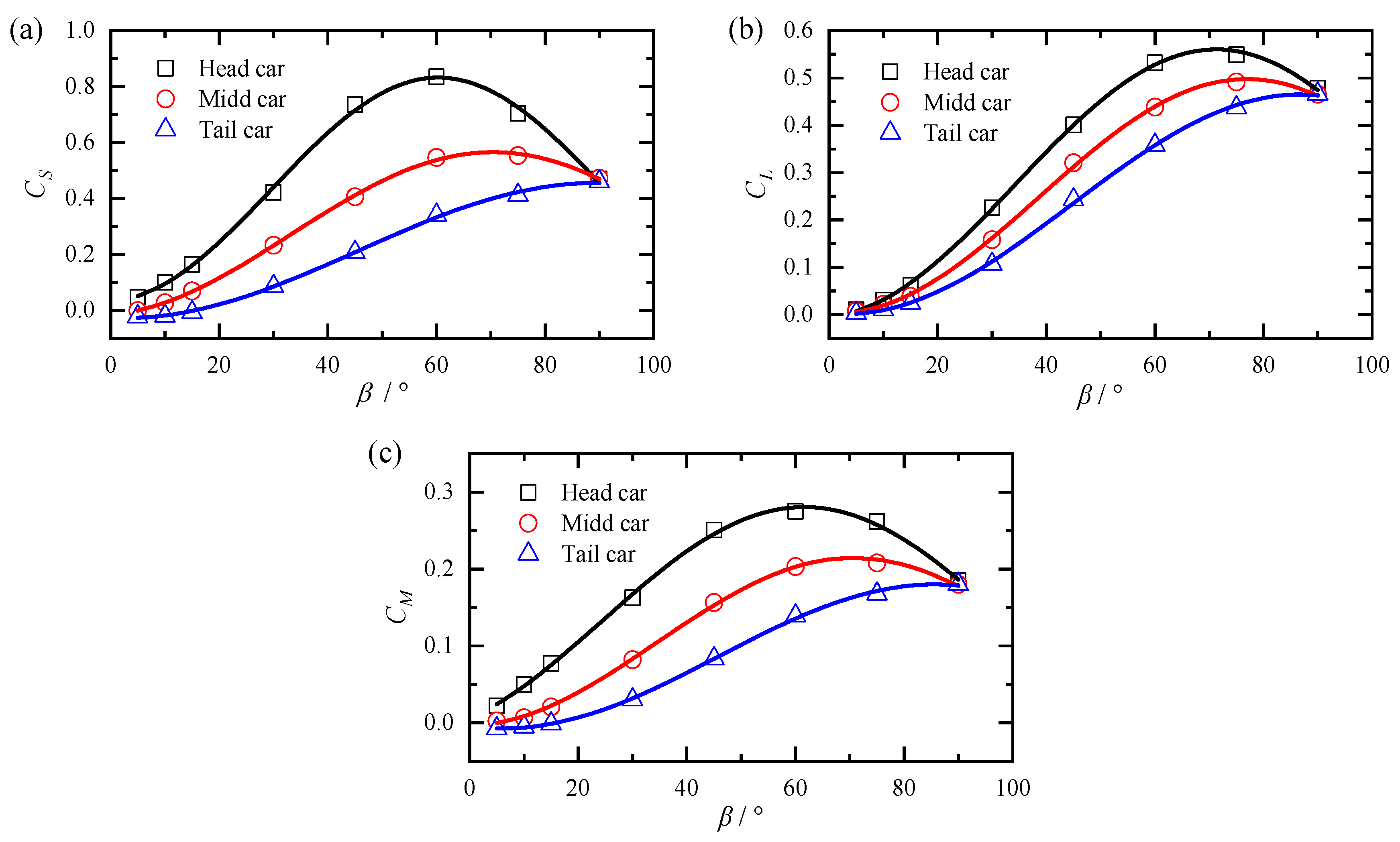
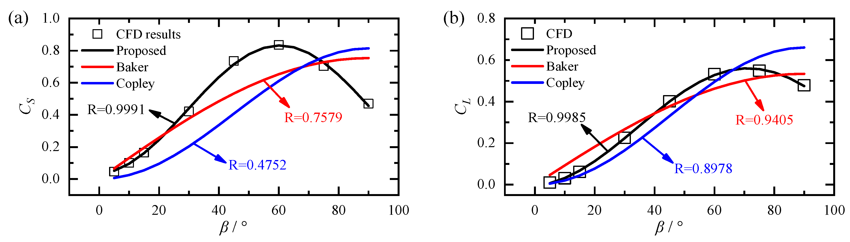
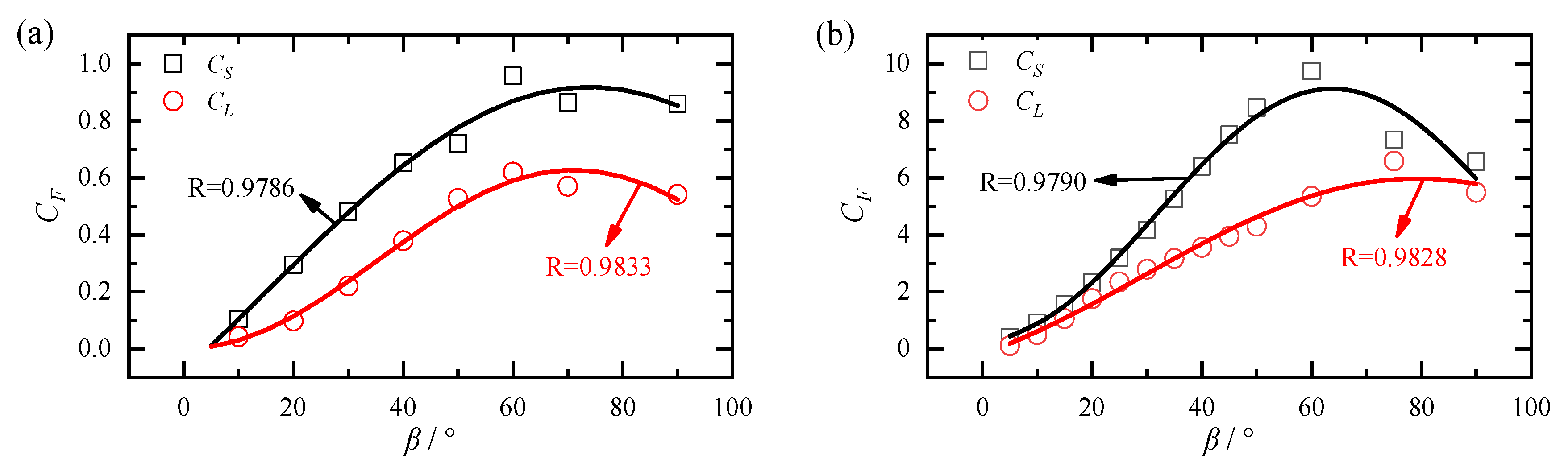
3.2. Aerodynamic Coefficients

Figure 11 shows the simulated aerodynamic coefficients of a moving train at the resultant yaw angle ranging from 0° to 90°. It is apparent that the aerodynamic coefficient of the head car is greater than that of the middle and tail cars. It is known from previous analysis that the flow structure of a moving train is featured by a three-dimensional characteristic due to the aerodynamic interaction between the train-induced wind and natural wind, which can be mapped onto the surface pressure distribution of the train along the length, leading to different forces on cars. Also, it can be found that the aerodynamic coefficient of the head and middle cars increases at low yaw angles but decreases at higher yaw angles. A similar trend also can be observed on the leading vehicle in terms of previous investigations [14,34]. However, it should be noted that there is a steady increase in the aerodynamic coefficient of the tail car as the yaw angle increases. In addition, the trend of the rolling coefficient in the resultant yaw angle is noticeably similar to that of the side coefficient, indicating that the rolling moment mainly results from the side force.

As discussed above, the resultant yaw angle is essential to the aerodynamic coefficient of a moving train. In general, it is a fact that when the train speed and wind speed with an incoming direction are given, we can obtain the corresponding aerodynamic coefficient of the train by calculating the resultant yaw angle. Thus, it is fundamental to explore the explicit expression between the resultant yaw angle and aerodynamic coefficient.

The experimental study carried out by Chiu and Squire [32] found that, the aerodynamic coefficient at large yaw angles follows the curve $C_F\left(\beta \right){=C}_F\left(90°\right)·{\sin }^2\left(\beta \right)$, where “F” means “S”, “L” or “R”, and $C_F\left(90°\right)$ is the force coefficient at 90° yaw angle. In the simulation of unsteady aerodynamic cross wind forces on trains, Baker [34] gave a crude approximation of the side and lift coefficient $C_F\left(\beta \right){=C}_F\left(90°\right)·\sin \left(\beta \right)$. Despite the fact that these expressions given by Chiu and Squire [32] and Baker [34] are quite simple and easy, they are not robust for a variety of vehicles. To solve this problem, this study attempts to propose a generalized prediction formula of the aerodynamic coefficient, expressed as follows:

$$C_F\left(\beta \right)=a+b\sin \left(c\beta +d\right)$$

(8)

where a, b, c, and d are the fitted parameters based on experimental or numerical data, respectively. With the use of the aerodynamic coefficient of the head car, Figure 12 plots the comparison results by means of different prediction formulas and

Table 1. The fitted parameters for the force coefficient of the head car.

Force Coefficient	Parameter
	a	b	c	d
CS	0.5016	−0.4643	0.0373	2.992
CL	0.2376	−0.2382	0.0997	2.141

lists the fitted coefficients. It is visible that Equation (8) can give a good agreement for the simulated side and lift coefficients when compared to the works by Chiu and Squire [32] and Baker [34], and the coefficient of determination R-squared, usually used to evaluate the fitting accuracy, is close to 1, implying that the prediction results are significantly reliable. A simple explanation for Equation (8) is that when the resultant wind speed is assumed to be a fixed value, the velocity component perpendicular to the car body and mainly determining the aerodynamic force on the train can be written by the sine function between V_R and β. Based on this, there may be a sinusoidal expression between the aerodynamic force coefficient and resultant angle.

In fact, the proposed prediction formula in Equation (8) is not only applicable to the aerodynamic coefficients of the train in this study, but also useful for most railway vehicles. Figure 13 depicts the prediction results of aerodynamic coefficients for different types of trains from the Advanced Passenger Train (APT) reported in the work by Baker [33] and ICE 3 leading vehicle given by European standard EN 14067-6 [44]. It can be seen that whether for the APT or ICE 3, the proposed aerodynamic prediction can agree well with the test results in the C_S and C_L, and the determination coefficients are above 0.97. In particular, at low resultant yaw angles, the prediction results are closely identical to the experimental data. Hence, we can deduct from the above results that a generalized sine prediction formula can be applied to most types of railway vehicles.

Besides, it should be noted that there is a higher cost in the proposed expression when compared to a simple perdition. In order to possibly reduce cost, it is suggested that at least four simulations or experiments should be carried out in actual use for the reason that there are four fitted coefficients in Equation (8).

Note that for the simulation of unsteady force with consideration of the vertical wind turbulence, the effect of the wind attack angle on the aerodynamic coefficient needs to be calculated. In order to economically obtain the aerodynamic data, it is assumed that the prediction formula in Equation (8) is also useful for the given wind attack angle. Thus, we can scale the aerodynamic curve at an attack angle of 0° to obtain the aerodynamic result for other attack angles by adopting the aerodynamic data at a resultant yaw angle of 90°. Although this method is a crude approximation, it is straightforward and practical for calculations. Figure 14 shows the side and lift coefficients of the head car at various attack angles using the approximate approach.

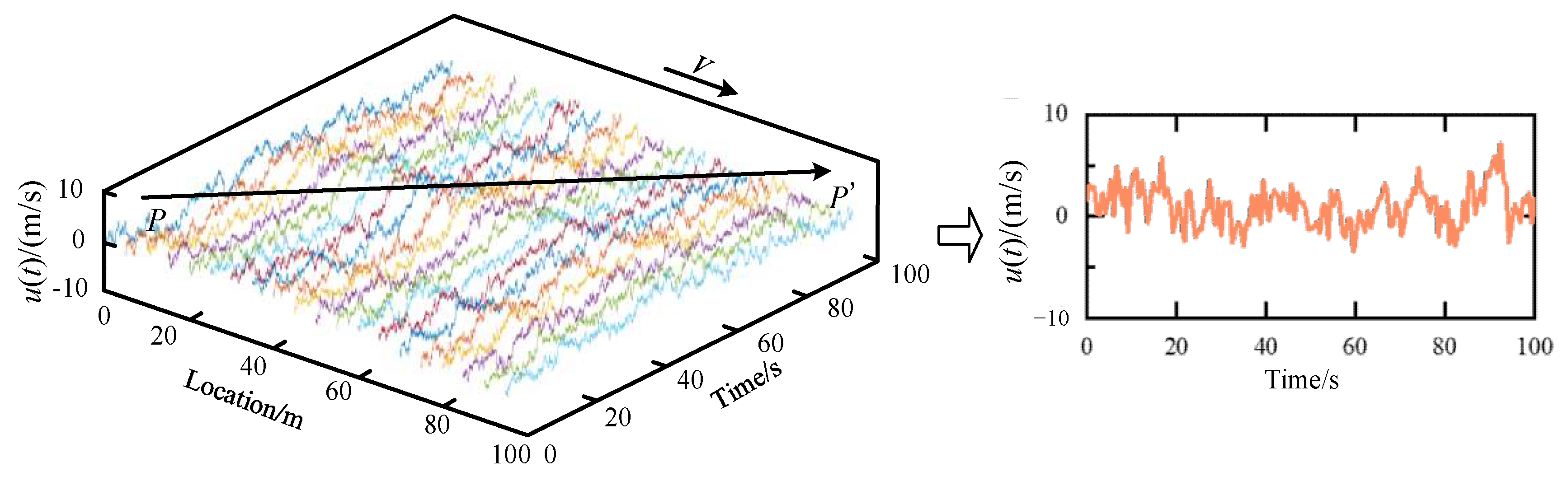
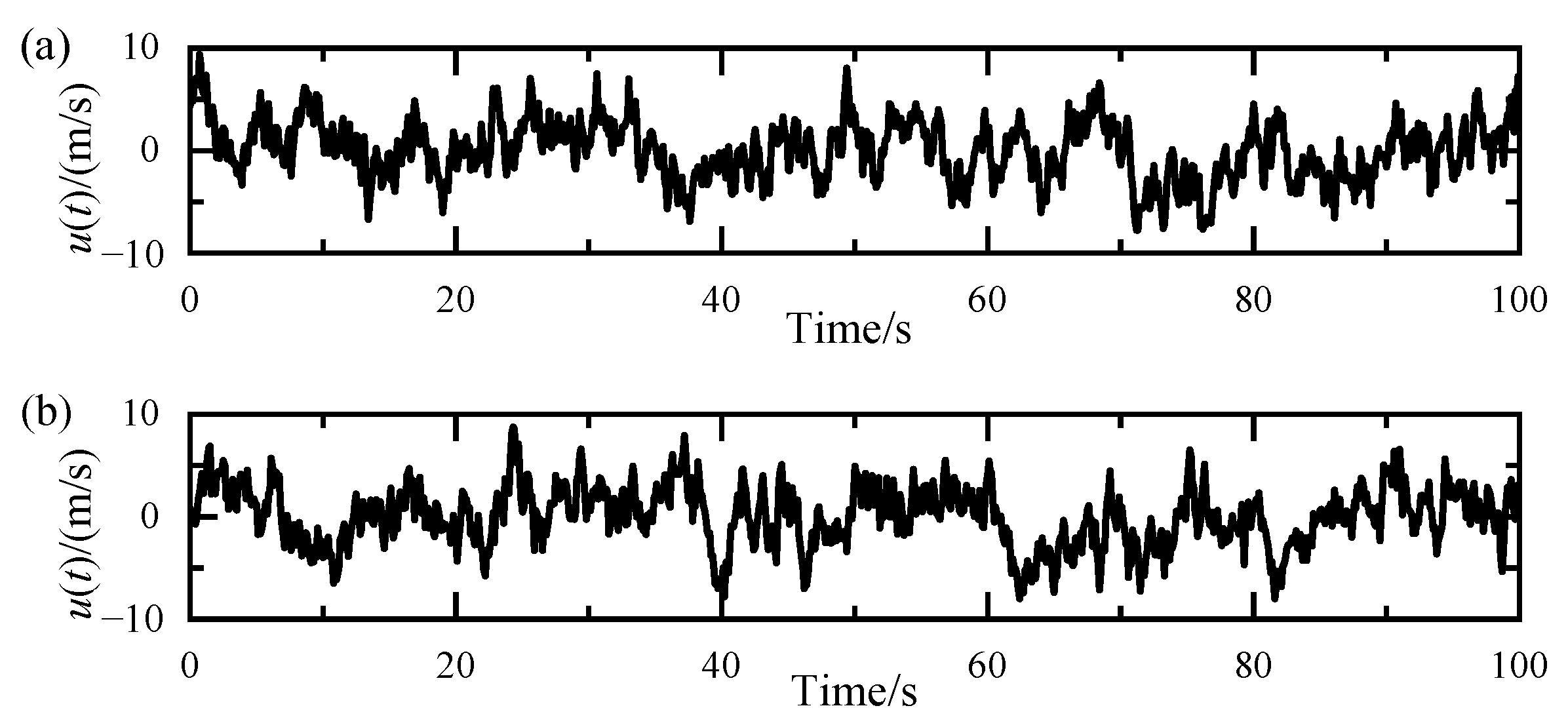
4. Wind Turbulence with Respect to a Moving Train

When a moving train is subjected to a crosswind, it will experience a three-dimensional stochastic wind field. Previous studies [3,14] had revealed that the fluctuating turbulence on a moving train is the time-space distribution, so it is a challenging and complicated procedure to obtain the stochastic wind turbulence. We will introduce two methods for calculating the fluctuating wind velocity at the position of a moving vehicle in this study: an interpolating method from artificially discrete simulated points (which is the stationary ergodic process) and a moving point simulation method based on Cooper’s theory.

The interpolating method from a large number of discrete points along the traveling track for simulating the fluctuating wind field on a moving vehicle had been used in previous researches by Xu et al. [4], Cheli et al. [14] and Montenegro et al. [8]. A typical example of this approach is described in Figure 15. As shown from the picture, when the vehicle moves from a point P in space to another point P′ at a constant speed of V, it is possible to obtain the wind velocity time series experienced by a moving vehicle using an interpolating algorithm between the adjacent discrete points on the track, which clearly reveals that the turbulent wind velocity on a moving train depends on time and location. The fundamental work of this method is to numerically generate the fluctuating wind velocity time histories of discrete points on the ground. In the present study, a fast-spectral representation method proposed by Cao et al. [45] is applied and thus the time histories of turbulent components u_j(t) at the point of j, can be expressed by:

$$u_j(t)=\sqrt{2\Delta \omega }{\displaystyle \sum _{m=1}^j{\displaystyle \sum _{k=1}^N\sqrt{S_u\left({\omega }_{mk}\right)}{G}_{jm}({\omega }_{mk})\cos ({\omega }_{mk}t+{\phi }_{mk})}}$$

(9)

where j = 1, 2, …, n1; n1 is the total number of simulated points; ∆ω is the frequency interval; N is the total number of frequency interval in the spectrum; S_u(ω) is the turbulent wind power spectral density (PSD); φ_mk is a random phase ranging between 0 and 2π; ω_mk = (k − 1)∆ω + m∆ω/n1; m = 1, 2, …, j; k = 1, 2, …, N; t is the time series in the simulation; and G(ω) is the coherence function. There is a significant advantage of the interpolating method that the spectral characteristic of turbulence on a moving train is the same as discrete points on the ground.

Although the interpolating approach is robust and easy to use, it is computationally intensive for a long traveling line where a large number of points along the track are used to divide the continuous wind field. To allow for this, an efficient solution was initially proposed by Cooper [35] to straightforwardly consider the spectral nature of wind turbulence on a running train in a crosswind through the hypothesis of Taylor’s frozen flow field and isotropic turbulence. Taking von Karman spectrum into account, Cooper [35] developed an analytical model of the fluctuating wind velocity spectrum with respect to a moving vehicle in the condition of a perpendicular wind direction, which had been applied in several researches by Baker [34], Yu et al. [36]. A numerical resolution with regard to Kaimal spectrum was performed by Wu et al. [37] and then, Li et al. [3], Yan et al. [38] and Hu et al. [39] proposed an analytical model for the different turbulence spectra with consideration of varying crosswind direction angles.

Figure 16 shows a diagram of a moving point and equivalent point in the application of Taylor’s frozen turbulence hypothesis. As the vehicle travels from P point at the time t to the P′ position at the time (t + τ) with a constant speed V, referring to Taylor’s hypothesis, the corresponding equivalent point P_e′ with regard to the P′ can be found in the frozen flow with a short duration time τ. Therefore, the cross-correlation coefficient functions between the P position and the P′ can be expressed by that of the P position and the P_e′, straightforwardly written as

$$\gamma \left({\Delta }_{P{P}^{\prime }},\tau \right)=\gamma \left({\Delta }_{P{P}_e^{\prime }},0\right)$$

(10)

where γ is the cross-correlation coefficient function; ∆ is the distance between two points in the spatial flow field. According to Equation (10), furthermore, the auto-correlation function can be calculated to obtain the power spectrum relative to a moving vehicle adopting the Fourier transform. The introductions of this method in detail were presented in the papers by Cooper [35], Wu et al. [37], Li et al. [3].

When the spectral density of a moving train is obtained, it is easy to calculate the wind velocity time series with the use of following expression:

$$u(t)=\sqrt{2\Delta \omega }{\displaystyle \sum _{k=1}^N\sqrt{S_u{}^M\left({\omega }_k\right)}\cos ({\omega }_{k}t+{\phi }_k)}$$

(11)

where S_u^M(ω) is the power spectra of a moving train, and the rest parameters remain the same as Equation (9). In contrast with the interpolating approach, the complex correlation characteristics of discrete points on the ground wind field need not to be generated in the moving point method, and thus the inefficient multivariable stochastic simulation can be simplified to a single random process to reduce the computing time and resource. The simulated longitudinal wind fluctuations of a moving train using two methods are shown in Figure 17. There are no significant differences in the simulated time series with the use of the interpolating method and the moving point algorithm.

From what has been described above, it is known that the simulation of unsteady wind velocity by a moving point scheme is more efficient in comparison with that of an interpolating method from a large number of artificial discrete fixed points. Nevertheless, it is necessary to be noted that there is a distinct limitation that the moving point method cannot consider the wind loads on the infrastructure where the vehicle travels. Previous investigations [4,8,40,46,47] revealed for the vehicle running on a bridge, the deflection and vibration from the bridge had significant impacts on the dynamic response of vehicles. The crosswind effect not only can act on the moving body but also on the bridge to form a complex coupled wind-vehicle-bridge system. Thus, the interpolating algorithm must be applied in such a case.

5. Unsteady Aerodynamic Forces Prediction with a Complete Turbulence

5.1. Prediction Model

When a complete turbulence field with a longitudinal component u(t), lateral component v(t), and vertical component w(t), is considered, the transient speed vectors on a moving train are drawn in Figure 18. It should be noted that the resultant wind speed V_R and yaw angle β are time-varying as a result of the fluctuating turbulence, which can be expressed by:

$$V_R=\overline{V_R}+{V_R}^{\prime }$$

(12)

$$\beta =\overline{\beta }+{\beta }^{\prime }+{\beta }^{″}$$

(13)

$$\overline{V_R}=\sqrt{{\left(V+U\cos \alpha \right)}^2+{\left(U\sin \alpha \right)}^2}$$

(14)

$$\overline{\beta }=\arctan \left(\frac{U\sin \alpha }{V+U\cos \alpha }\right)$$

(15)

where $\overline{V_R}$ and ${V_R}^{\prime }$ are the mean component and the fluctuating component of the resultant wind speed, respectively; $\overline{\beta }$ is the mean component of the resultant wind yaw angle; ${\beta }^{\prime }$ and ${\beta }^{″}$ are the fluctuating components resulting from the longitudinal turbulence u(t) and lateral turbulence v(t), respectively. Noting that the resultant wind speed also can be given in terms of the geometrical relations shown in Figure 18:

$$V_R{}^2={\left[V+\left(U+u\right)\cos \alpha +v\sin \alpha \right]}^2+{\left[(U+u)\sin \alpha -v\cos \alpha \right]}^2+w^2$$

(16)

It is assumed that the train speed V and wind speed U are significantly greater than the fluctuating components. Neglecting the high-order fluctuations of wind turbulence, an approximate expression from Equations (12), (14) and (16) can be obtained:

$$V_R{}^2\approx {\overline{V_R}}^2+2\overline{V_R}{V_R}^{\prime }\approx {\overline{V_R}}^2+2u\left(U+V\cos \alpha \right)+2Vv\sin \alpha$$

(17)

Thus, the fluctuation turbulence on a moving train can be written as

$${V_R}^{\prime }\approx \frac{\left(U+V\cos \alpha \right)u+Vv\sin \alpha }{\overline{V_R}}$$

(18)

It can be seen from Equation (18) that the resultant wind turbulence of a moving train depends on the longitudinal and lateral turbulence. It should be noted that the following geometrical relations are possible to be observed from Figure 18:

$$\left\{\begin{array}{l}\cos \left(\alpha -\overline{\beta }\right)=\frac{U+V\cos \alpha }{\overline{V_R}}\\ \sin \left(\alpha -\overline{\beta }\right)=\frac{V\sin \alpha }{\overline{V_R}}\end{array}\right.$$

(19)

Hence, an equivalent expression of Equation (17) can be obtained

$${V_R}^{\prime }\approx u\cos \left(\alpha -\overline{\beta }\right)+v\sin \left(\alpha -\overline{\beta }\right)$$

(20)

Based on the quasi-steady hypothesis, the unsteady aerodynamic forces F of a moving vehicle, consisting of a mean $\overline{F}$ and a fluctuation $F^{\prime }$, can be expressed by a mean resultant speed $\overline{V_R}$ and a fluctuating resultant speed ${V_R}^{\prime }$:

$$F=\overline{F}+F^{\prime }=0.5\rho A{C}_F\left(\beta ,\theta \right){\left(\overline{V_R}+{V_R}^{\prime }\right)}^2$$

(21)

Through Taylor series expansion at θ = 0 and $\beta =\overline{\beta }$, the aerodynamic coefficient can be written as an approximate expression:

$$C_F\left(\theta ,\beta \right)\approx C_F\left(\overline{\beta },0\right)+{\left.\frac{\partial C_F}{\partial \beta }\right|}_{\begin{array}{l}\theta =0\\ \beta =\overline{\beta }\end{array}}\left({\beta }^{\prime }+{\beta }^{″}\right)+{\left.\frac{\partial C_F}{\partial \theta }\right|}_{\begin{array}{l}\theta =0\\ \beta =\overline{\beta }\end{array}}\theta$$

(22)

The following simplification is utilized for the sake of the easy writing:

$$C_F\left(\beta ,\theta \right)\approx C_F\left(\overline{\beta }\right)+{C_F}^{\prime }\left(\overline{\beta }\right)\left({\beta }^{\prime }+{\beta }^{″}\right)+{C_F}^{\prime }\left(0\right)\theta$$

(23)

Due to the small longitudinal and lateral turbulence, the fluctuation of a resultant yaw angle can be approximated:

$${\beta }^{\prime }+{\beta }^{″}\approx \sin \left(\beta -\overline{\beta }\right)=\sin \beta \cos \overline{\beta }-\cos \beta \sin \overline{\beta }$$

(24)

Referring to Figure 18, it is easy to be found:

$$\left\{\begin{array}{l}\sin \overline{\beta }=\frac{U\sin \alpha }{\overline{V_R}}\\ \cos \overline{\beta }=\frac{V+U\cos \alpha }{\overline{V_R}}\\ \sin \beta =\frac{\left(U+u\right)\sin \alpha -v\cos \alpha }{\overline{V_R}+{V_R}^{\prime }}\\ \cos \beta =\frac{V+\left(U+u\right)\cos \alpha +v\sin \alpha }{\overline{V_R}+{V_R}^{\prime }}\end{array}\right.$$

(25)

Equations (24) and (25) lead to

$${\beta }^{\prime }+{\beta }^{″}\approx \frac{u\sin \left(\alpha -\overline{\beta }\right)-v\cos \left(\alpha -\overline{\beta }\right)}{\overline{V_R}}$$

(26)

It is clear that the lateral turbulence contributes to a negative effect on the resultant fluctuating yaw angle. The small attack angle θ is probably calculated by

$$\theta \approx \sin \theta \approx \frac{w}{\overline{V_R}}$$

(27)

Substituting Equations (18), (23), (26) and (27) into Equation (21), the unsteady aerodynamic force of a moving train in a complete turbulence field can be written as:

$$\begin{array}{ll}F& =\overline{F}+F^{\prime }=\overline{F}+{F_u}^{\prime }+{F_v}^{\prime }+{F_w}^{\prime }\\ & \approx \frac{1}{2}\rho A{C}_F\left(\overline{\beta }\right){\overline{V_R}}^2+\frac{1}{2}\rho A{C}_u\overline{V_R}u+\frac{1}{2}\rho A{C}_v\overline{V_R}v+\frac{1}{2}\rho A{C}_w\overline{V_R}w\end{array}$$

(28)

where

$$\left\{\begin{array}{l}{C}_u=2C_F\left(\overline{\beta }\right)\cos \left(\alpha -\overline{\beta }\right)+{C_F}^{\prime }\left(\overline{\beta }\right)\sin \left(\alpha -\overline{\beta }\right)\\ C_v=2C_F\left(\overline{\beta }\right)\sin \left(\alpha -\overline{\beta }\right)-{C_F}^{\prime }\left(\overline{\beta }\right)\cos \left(\alpha -\overline{\beta }\right)\\ C_w={C_F}^{\prime }\left(0\right)\end{array}\right.$$

(29)

${F_u}^{\prime }$, ${F_v}^{\prime }$, and ${F_w}^{\prime }$ are the fluctuating value caused by the longitudinal, lateral, and vertical turbulence, respectively.

When only the longitudinal turbulence u(t) is included and crosswind is perpendicular to the traveling line (α = 90°), the fluctuating value with respect to unsteady force can be simplified as follows:

$$F^{\prime }=\frac{1}{2}\rho A\left[2C_F\left(\overline{\beta }\right)\sin \left(\overline{\beta }\right)+{C_F}^{\prime }\left(\overline{\beta }\right)\cos \left(\overline{\beta }\right)\right]\overline{V_R}u$$

(30)

which is an equivalent form proposed by Baker [34]. For a case where the longitudinal turbulence u(t) and vertical turbulence w(t) are concerned, and assume β′ = 0 and α = 90°, it can lead to:

$$F^{\prime }=\frac{1}{2}\rho A\overline{V_R}\left[2C_F\left(\overline{\beta }\right)\sin \left(\overline{\beta }\right)u+{C_F}^{\prime }\left(0\right)w\right]$$

(31)

which is similar to the results by Li et al. [40]. While the fluctuating turbulence u(t) and v(t) are taken into account, we can obtain the same results by Yu et al. [36].

It should be mentioned that force fluctuation through the use of the quasi-steady theory fully follows the velocity fluctuation. In reality, this assertion does not hold completely since the shape and suspension characteristics of vehicles are able to filter out some small scales and high frequency turbulences [34,48,49]. To allow for this the aerodynamic weighting function h_F(τ) approach is used to relate the instantaneous variations from force to wind velocity in the time domain. The fluctuating component in Equation (28) is corrected by

$$F^{\prime }=\frac{1}{2}\rho A\overline{V_R}\left[C_u{\displaystyle {\int }_0^{\infty }{h}_F(\tau )u(t-\tau )d\tau }+C_v{\displaystyle {\int }_0^{\infty }{h}_F(\tau )v(t-\tau )d\tau +C_w{\displaystyle {\int }_0^{\infty }{h}_F(\tau )w(t-\tau )d\tau }}\right]$$

(32)

The weighting function can be obtained by the aerodynamic admittance function X_F(ω) in frequency domain through a Fourier transform

$$h_F(\tau )={\displaystyle {\int }_0^{\infty }\left|X_F(\omega )\right|}{e}^{2\pi \omega i}d\omega$$

(33)

where ω is the frequency in Hz and i is the square root of −1. In practice the admittance function is a ratio of the force spectrum $S_F\left(\omega \right)$ to the wind spectrum $S_W\left(\omega \right)$, in general measured through by means of a series of scaled wind tunnel experiments [48,49] or full-scale field tests [13], defined as:

$${\left|{{\rm X}}_F\left(\omega \right)\right|}^2=\frac{1}{{\left(\rho A{C}_F\overline{V_R}\right)}^2}\frac{S_F\left(\omega \right)}{S_W\left(\omega \right)}$$

(34)

Through a large amount of experimental data, Sterling et al. [48] parameterized an approximate expression of the admittance function in regard to railway vehicles. Baker [34] further facilitated the admittance function form and derived the weighting function expression in time domain:

$$h_F\left(\overline{\tau }\right)={\left(2\pi \overline{n^{\prime }}\right)}^2\overline{\tau }{e}^{-2\pi \overline{n^{\prime }}\overline{\tau }}$$

(35)

where $\overline{\tau }$ is the reduced time ($\overline{\tau }=\tau U/l$, l is the length of car body); $\overline{n^{\prime }}$ is a fitting parameter from available experimental data, approximately given by

$$\overline{n^{\prime }}=\gamma \sin \overline{\beta }$$

(36)

γ = 2.0 for side force and γ = 2.5 for lift force.

5.2. Case Study

With the use of aerodynamic parameters described above and taking the head car as an example, Figure 19 plots the simulated unsteady aerodynamic forces time histories of a moving train about 100 s by means of the quasi-steady calculation and the weighting function approach. It is obvious that the fluctuating parts of unsteady side and lift forces always oscillate up and down around the mean value, which is to be expected as the aerodynamic force is derived from the fluctuating time series swinging around the mean wind velocity. According to the definition of unsteady force in Equation (32), it can be found that the significant difference between the quasi-steady approach and the weighting function approach is how fluctuation in the turbulence leads to variation in the force. It is clear from Figure 19 that the side and lift force curves through the weighting function approach are smoother for the reason that some high frequency turbulences are filtered. In addition, the unsteady force in the weighting function exhibits a slight time lag in comparison with the quasi-steady result, which follows the turbulence fluctuation exactly. Note that the following discussion of unsteady force will be based on the result obtained from the weighting function method.

When the train speed and wind speed are given, the varying crosswind direction can lead to impacts on the aerodynamic coefficient and resultant wind speed to affect the unsteady loads of a moving train. Figure 20 shows the effect of crosswind direction on the mean side force. It clearly illustrates that the increasing crosswind angle brings out an increase in the mean component of unsteady force firstly and then a decrease, and the corresponding maximum appears around 80°–90° incoming flow direction of crosswind that is approximately perpendicular to the travel line, which is possible to be unfavorable to the train’s stability.

Figure 21 shows the simulated side force time histories at three typical crosswind directions (30°, 90°, 150°) to explore different wind turbulence effects on the unsteady force. Observing the results at 90° wind direction, we can see that the unsteady force time series resulting from both longitudinal and lateral turbulences are similar to the results only including the longitudinal turbulence, indicating there is no visible effect of lateral turbulence on the force fluctuation. However, at conditions of 30° and 150° crosswind angles, it is clearly visible that the longitudinal, lateral and vertical turbulence can considerably contribute to the unsteady force curves. One explanation might simply be that when the crosswind direction swings around 90°, lateral turbulence is approximately parallel to the moving direction of the vehicle, which can only contribute to less effective turbulent components normal to the car-body to produce small fluctuation in the force. Besides, it also can be found that the wind turbulence in the vertical direction has a great impact on the unsteady force throughout the crosswind direction because it is always normal to the moving train.

The extreme value of unsteady force, in general, related to the extreme index used to assess the running safety and ride quality of railway vehicles, is of great importance. Considering different wind turbulences and using simulated 100s realizations of the unsteady force time series, Figure 22 shows the ratio of the maximum value to the mean. We can see from Figure 22a that as train speed increases, the force peak value/mean ratio decreases steadily, and the result including the complete wind turbulence is significantly larger, implying that considering only part of turbulence in the simulation of unsteady force perhaps underestimate the crosswind effect on vehicle stability. Also, for the varying crosswind direction, we can obtain from Figure 22b the maximum peak/mean ratio in a complete turbulence field. On the other hand, with the increasing crosswind direction, the variation of peak/mean ratio caused by the longitudinal turbulence is similar to that of the mean force, namely increasing firstly and then decreasing, and the maximum being near 90° crosswind angle. As discussed above, the lateral turbulence has almost no impact on the peak/mean ratio around 90° crosswind angle. Nevertheless, for cases far away from 90° crosswind direction, the effect of the lateral turbulence on the peak/mean ratio cannot be neglected. Especially for high incoming flow direction of crosswind, the peak/mean ratio is significantly dominated by the lateral turbulence.

6. Conclusions and Further Works

Aerodynamic forces are significantly essential to the dynamic response analysis and overturning risk assessment of trains in crosswinds. Starting with the simulation of aerodynamic characteristics using the CFD method, an analytical model for predicting unsteady aerodynamic forces of a moving train subjected to a crosswind was set out in this study. Compared to the conventional approach widely used in previous investigations, the newly proposed model can capture the effects of both three-dimensional wind turbulence and varying flow direction of natural wind. The following conclusions can be drawn:

(1)

The flow pattern of a moving train exposed to a crosswind is characterized by three-dimensional structures on account of the aerodynamic coupling effect of the train-induced wind and crosswind, and it is mainly determined by the resultant wind speed V_R and yaw angle β, related to the train speed V and wind speed U with a flow angle of α.

(2)

A generalized sine expression can be used to predict the aerodynamic coefficient of a moving train varying with the resultant wind yaw angle, and based on wind tunnel test data, it is proved that the prediction formula is possible to be applied to most types of trains.

(3)

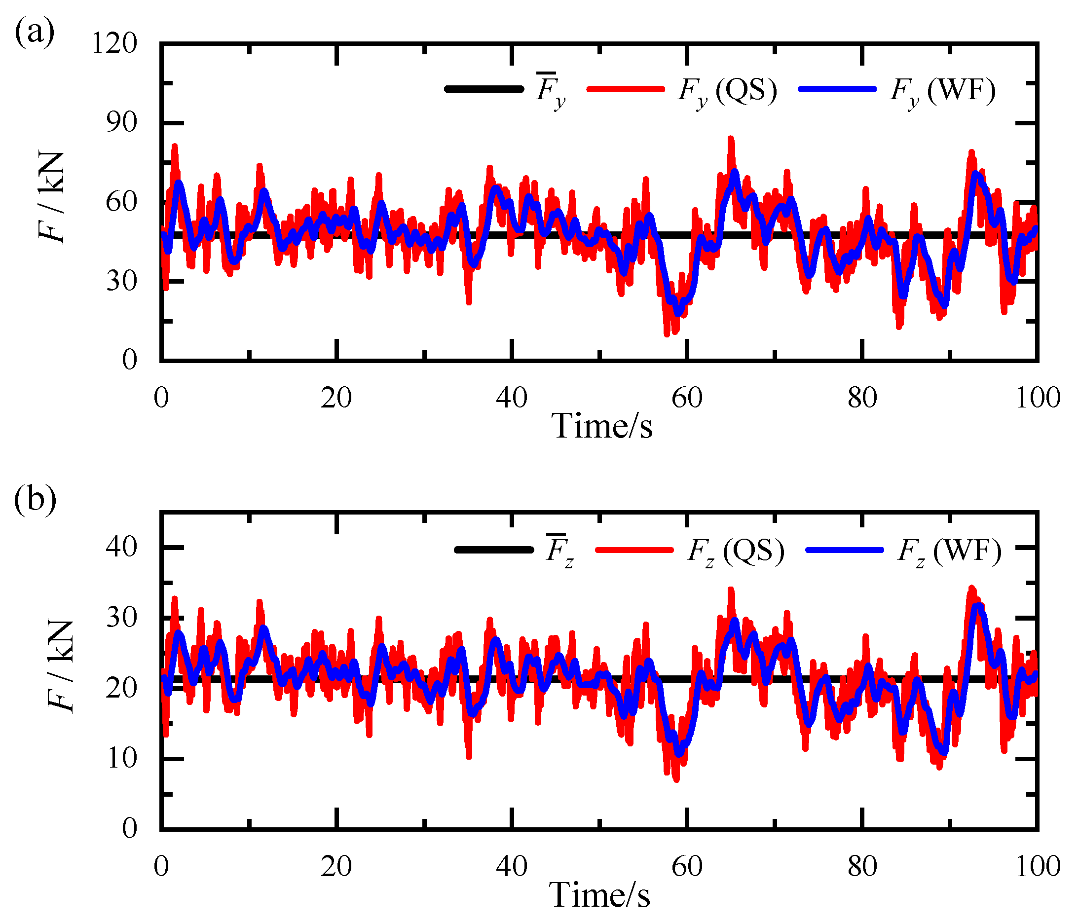
The quasi-steady and weighting function methods are developed through a mathematical process to calculate unsteady aerodynamic forces of a moving vehicle in a three-dimensional stochastic wind field, which shows good agreements with previous models. Moreover, the filtering and time lag effects are found in the weighting function approach.

(4)

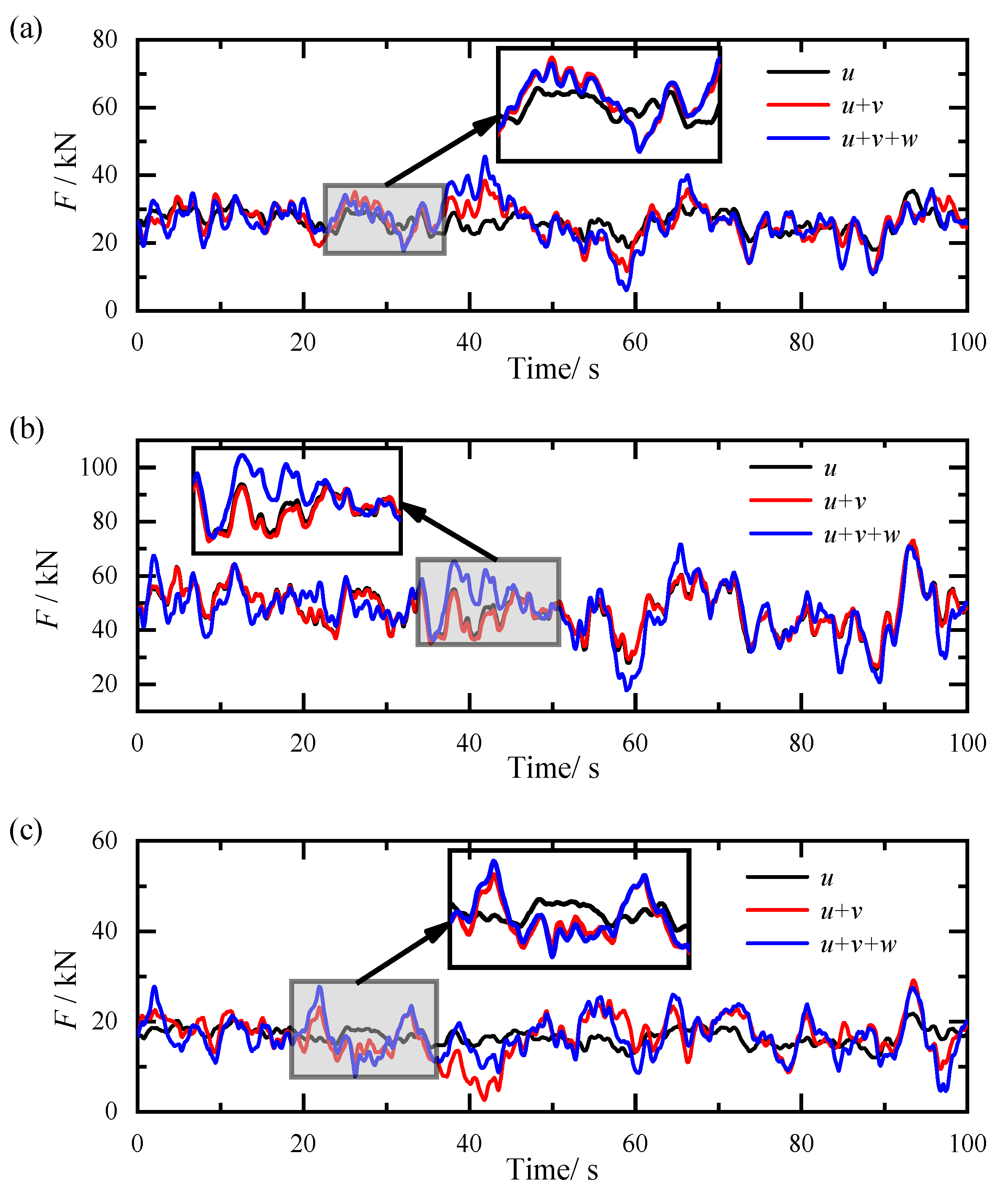
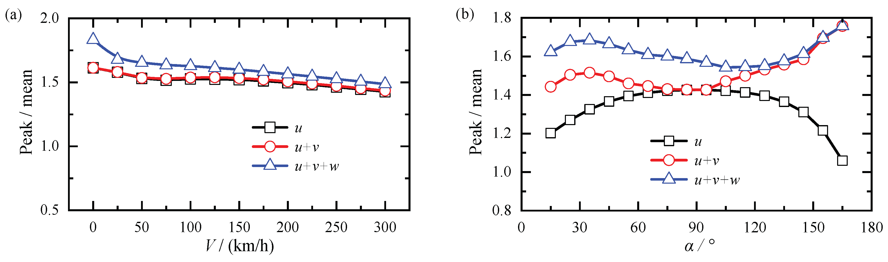
When the complete wind turbulence is considered, greater force fluctuation and peak can be found, and also, variations in the wind direction are crucial to unsteady aerodynamic forces of moving trains, which can lead to maximum mean force at approximately 90° wind direction. However, when the flow direction of crosswind deviates from 90°, consideration of only a portion of the turbulence components may underestimate the dynamic response of trains.

Our next work is the use of the simulated results to calculate the dynamic responses of trains in crosswinds with considerations of the track irregularity, track defects, foundation settlement, etc., which can also give some significant suggestions for the optimization and design of trains. Moreover, the simulated forces are useful in being applied to determine the characteristic wind curves of trains through a dynamic multi-body simulation. However, we acknowledge that some fundamental issues in the simulation remain to be explored and studied in further research, for example, the determination of aerodynamic admittance function.

References

- Andersson, E.; Häggström, J.; Sima, M.; Stichel, S. Assessment of train-overturning risk due to strong cross-winds. Proc. Inst. Mech. Eng. Part F J. Rail Rapid Transit 2004, 218, 213–223. [Google Scholar] [CrossRef]
- Baker, C.; Cheli, F.; Orellano, A.; Paradot, N.; Proppe, C.; Rocchi, D. Cross-wind effects on road and rail vehicles. Veh. Syst. Dyn. 2009, 47, 983–1022. [Google Scholar] [CrossRef]
- Li, X.; Xiao, J.; Liu, D.; Wang, M.; Zhang, D. An analytical model for the fluctuating wind velocity spectra of a moving vehicle. J. Wind Eng. Ind. Aerodyn. 2017, 164, 34–43. [Google Scholar] [CrossRef]
- Xu, Y.; Ding, Q. Interaction of railway vehicles with track in cross-winds. J. Fluids Struct. 2006, 22, 295–314. [Google Scholar] [CrossRef]
- Zhai, W.; Yang, J.; Li, Z.; Han, H. Dynamics of high-speed train in crosswinds based on an air-train-track interaction model. Wind Struct. 2015, 20, 143–168. [Google Scholar] [CrossRef]
- Baker, C. Risk analysis of pedestrian and vehicle safety in windy environments. J. Wind Eng. Ind. Aerodyn. 2015, 147, 283–290. [Google Scholar] [CrossRef]
- He, X.; Shi, K.; Wu, T. An efficient analysis framework for high-speed train-bridge coupled vibration under non-stationary winds. Struct. Infrastruct. Eng. 2020, 16, 1326–1346. [Google Scholar] [CrossRef]
- Montenegro, P.; Barbosa, D.; Carvalho, H.; Calçada, R. Dynamic effects on a train-bridge system caused by stochastically generated turbulent wind fields. Eng. Struct. 2020, 211, 110430. [Google Scholar] [CrossRef]
- Neto, J.; Montenegro, P.; Vale, C.; Calçada, R. Evaluation of the train running safety under crosswinds-a numerical study on the influence of the wind speed and orientation considering the normative Chinese Hat Model. Int. J. Rail Transp. 2021, 9, 204–231. [Google Scholar] [CrossRef]
- Yao, Z.; Zhang, N. Overturning assessment of railway vehicles under cross winds. Wind Struct. 2021, 33, 1–11. [Google Scholar] [CrossRef]
- Han, Y.; Zhang, X.; Wang, L.; Zhu, Z.; Cai, C.S.; He, X. Running Safety Assessment of a Train Traversing a Long-Span Bridge Under Sudden Changes in Wind Loads Owing to Damaged Wind Barriers. Int. J. Struct. Stab. Dyn. 2022, 22, 2241010. [Google Scholar] [CrossRef]
- Wang, M.; Li, X.; Chen, X. A simplified analysis framework for assessing overturning risk of high-speed trains over bridges under crosswind. Veh. Syst. Dyn. 2022, 60, 1037–1047. [Google Scholar] [CrossRef]
- Baker, C.; Jones, J.; Lopez-Calleja, F.; Munday, J. Measurements of the cross wind forces on trains. J. Wind Eng. Ind. Aerodyn. 2004, 92, 547–563. [Google Scholar] [CrossRef]
- Cheli, F.; Ripamonti, F.; Rocchi, D.; Tomasini, G. Aerodynamic behaviour investigation of the new EMUV250 train to cross wind. J. Wind Eng. Ind. Aerodyn. 2010, 98, 189–201. [Google Scholar] [CrossRef]
- Yao, Z.; Zhang, N.; Chen, X.; Zhang, C.; Xia, H.; Li, X. The effect of moving train on the aerodynamic performances of train-bridge system with a crosswind. Eng. Appl. Comput. Fluid Mech. 2020, 14, 222–235. [Google Scholar] [CrossRef]
- Li, X.; Tan, Y.; Qiu, X.; Gong, Z.; Wang, M. Wind tunnel measurement of aerodynamic characteristics of trains passing each other on a simply supported box girder bridge. Railw. Eng. Sci. 2021, 29, 152–162. [Google Scholar] [CrossRef]
- Wu, J.; Li, X.; Cai, C.S.; Liu, D. Aerodynamic characteristics of a high-speed train crossing the wake of a bridge tower from moving model experiments. Railw. Eng. Sci. 2022, 30, 221–241. [Google Scholar] [CrossRef]
- Li, Y.; Hu, P.; Xu, Y.; Zhang, M.; Liao, H. Wind loads on a moving vehicle-bridge deck system by wind-tunnel model test. Wind Struct. 2014, 19, 145–167. [Google Scholar] [CrossRef]
- Xiang, H.; Li, Y.; Chen, S.; Hou, G. Wind loads of moving vehicle on bridge with solid wind barrier. Eng. Struct. 2018, 156, 188–196. [Google Scholar] [CrossRef]
- Li, X.; Wang, M.; Xiao, J.; Zou, Q.; Liu, D. Experimental study on aerodynamic characteristics of high-speed train on a truss bridge: A moving model test. J. Wind Eng. Ind. Aerodyn. 2018, 179, 26–38. [Google Scholar] [CrossRef]
- He, X.; Zou, S. Crosswind effects on a train-bridge system: Wind tunnel tests with a moving vehicle. Struct. Infrastruct. Eng. 2021, 1–13. [Google Scholar] [CrossRef]
- Hu, Y.; Xu, F.; Gao, Z. A Comparative Study of the Simulation Accuracy and Efficiency for the Urban Wind Environment Based on CFD Plug-Ins Integrated into Architectural Design Platforms. Buildings 2022, 12, 1487. [Google Scholar] [CrossRef]
- Song, J.L.; Li, J.W.; Xu, R.Z.; Flay, R.G. Field measurements and CFD simulations of wind characteristics at the Yellow River bridge site in a converging-channel terrain. Eng. Appl. Comput. Fluid Mech. 2022, 16, 58–72. [Google Scholar] [CrossRef]
- Rizzo, F.; D’Alessandro, V.; Montelpare, S.; Giammichele, L. Computational study of a bluff body aerodynamics: Impact of the laminar-to-turbulent transition modelling. Int. J. Mech. Sci. 2020, 178, 105620. [Google Scholar] [CrossRef]
- Sun, Z.; Yao, S.; Wei, L.; Yao, Y.; Yang, G. Numerical investigation on the influence of the streamlined structures of the high-speed train’s nose on aerodynamic performances. Appl. Sci. 2021, 11, 784. [Google Scholar] [CrossRef]
- Yan, J.; Chen, T.; Deng, E.; Yang, W.; Cheng, S.; Zhang, B. Aerodynamic Response and Running Posture Analysis When the Train Passes a Crosswind Region on a Bridge. Appl. Sci. 2021, 11, 4126. [Google Scholar] [CrossRef]
- Zou, S.; He, X.; Wang, H. Numerical investigation on the crosswind effects on a train running on a bridge. Eng. Appl. Comput. Fluid Mech. 2020, 14, 1458–1471. [Google Scholar] [CrossRef]
- Chen, Z.W.; Rui, E.Z.; Liu, T.H.; Ni, Y.Q.; Huo, X.S.; Xia, Y.T.; Li, W.H.; Guo, Z.J.; Zhou, L. Unsteady Aerodynamic Characteristics of a High-Speed Train Induced by the Sudden Change of Windbreak Wall Structure: A Case Study of the Xinjiang Railway. Appl. Sci. 2022, 12, 7217. [Google Scholar] [CrossRef]
- Wang, B.; Xu, Y.; Zhu, L.; Li, Y. Crosswind effect studies on road vehicle passing by bridge tower using computational fluid dynamics. Eng. Appl. Comput. Fluid Mech. 2014, 8, 330–344. [Google Scholar] [CrossRef]
- Wang, M.; Li, X.; Xiao, J.; Zou, Q.; Sha, H. An experimental analysis of the aerodynamic characteristics of a high-speed train on a bridge under crosswinds. J. Wind Eng. Ind. Aerodyn. 2018, 177, 92–100. [Google Scholar] [CrossRef]
- Wang, Y.; Xia, H.; Guo, W.; Zhang, N.; Wang, S. Numerical analysis of wind field induced by moving train on HSR bridge subjected to crosswind. Wind Struct. 2018, 27, 29–40. [Google Scholar] [CrossRef]
- Chiu, T.; Squire, L. An experimental study of the flow over a train in a crosswind at large yaw angles up to 90. J. Wind Eng. Ind. Aerodyn. 1992, 45, 47–74. [Google Scholar] [CrossRef]
- Baker, C. Ground vehicles in high cross winds part I: Steady aerodynamic forces. J. Fluids Struct. 1991, 5, 69–90. [Google Scholar] [CrossRef]
- Baker, C. The simulation of unsteady aerodynamic cross wind forces on trains. J. Wind Eng. Ind. Aerodyn. 2010, 98, 88–99. [Google Scholar] [CrossRef]
- Cooper, R. Atmospheric turbulence with respect to moving ground vehicles. J. Wind Eng. Ind. Aerodyn. 1984, 17, 215–238. [Google Scholar] [CrossRef]
- Yu, M.; Liu, J.; Liu, D.; Chen, H.; Zhang, J. Investigation of aerodynamic effects on the high-speed train exposed to longitudinal and lateral wind velocities. J. Fluids Struct. 2016, 61, 347–361. [Google Scholar] [CrossRef]
- Wu, M.; Li, Y.; Chen, X.; Hu, P. Wind spectrum and correlation characteristics relative to vehicles moving through cross wind field. J. Wind Eng. Ind. Aerodyn. 2014, 133, 92–100. [Google Scholar] [CrossRef]
- Yan, N.; Chen, X.; Li, Y. Assessment of overturning risk of high-speed trains in strong crosswinds using spectral analysis approach. J. Wind Eng. Ind. Aerodyn. 2018, 174, 103–118. [Google Scholar] [CrossRef]
- Hu, P.; Han, Y.; Cai, C.; Cheng, W.; Lin, W. New analytical models for power spectral density and coherence function of wind turbulence relative to a moving vehicle under crosswinds. J. Wind Eng. Ind. Aerodyn. 2019, 188, 384–396. [Google Scholar] [CrossRef]
- Li, Y.; Qiang, S.; Liao, H.; Xu, Y. Dynamics of wind-rail vehicle-bridge systems. J. Wind Eng. Ind. Aerodyn. 2005, 93, 483–507. [Google Scholar] [CrossRef]
- Cheli, F.; Corradi, R.; Tomasini, G. Crosswind action on rail vehicles: A methodology for the estimation of the characteristic wind curves. J. Wind Eng. Ind. Aerodyn. 2012, 104–106, 248–255. [Google Scholar] [CrossRef]
- Sha, H. Aerodynamic Characteristics of Simply Supported Beam High Speed Train System under Crosswinds. Master’s Thesis, Southwest Jiaotong University, Chendu, China, 2019. [Google Scholar]
- Copley, J. The three-dimensional flow around railway trains. J. Wind Eng. Ind. Aerodyn. 1987, 26, 21–52. [Google Scholar] [CrossRef]
- EN 14067-6; Railway Applications Aerodynamics Part 6: Requirements and Test Procedures for Cross Wind Assessment. CEN: Brussels, Belgium, 2018.
- Cao, Y.; Xiang, H.; Zhou, Y. Simulation of stochastic wind velocity field on long-span bridges. J. Eng. Mech. 2000, 126, 1–6. [Google Scholar] [CrossRef]
- Cai, C.; Hu, J.; Chen, S.; Han, Y.; Zhang, W.; Kong, X. A coupled wind-vehicle-bridge system and its applications: A review. Wind Struct. 2015, 20, 117–142. [Google Scholar] [CrossRef] [Green Version]
- Olmos, J.M.; Astiz, M.A. Improvement of the lateral dynamic response of a high pier viaduct under turbulent wind during the high-speed train travel. Eng. Struct. 2018, 165, 368–385. [Google Scholar] [CrossRef]
- Sterling, M.; Baker, C.; Bouferrouk, A.; ONeil, H.; Wood, S.; Crosbie, E. An investigation of the aerodynamic admittances and aerodynamic weighting functions of trains. J. Wind Eng. Ind. Aerodyn. 2009, 97, 512–522. [Google Scholar] [CrossRef] [Green Version]
- Tomasini, G.; Cheli, F. Admittance function to evaluate aerodynamic loads on vehicles: Experimental data and numerical model. J. Fluids Struct. 2013, 38, 92–106. [Google Scholar] [CrossRef]