Abstract
Elevating the accuracy of streamflow forecasting has always been a challenge. This paper proposes a three-step artificial intelligence model improvement for streamflow forecasting. Step 1 uses long short-term memory (LSTM), an improvement on the conventional artificial neural network (ANN). Step 2 performs multi-step ahead forecasting while establishing the rates of change as a new approach. Step 3 further improves the accuracy through three different kinds of optimization algorithms. The Stormwater and Road Tunnel project in Kuala Lumpur is the study area. Historical rainfall data of 14 years at 11 telemetry stations are obtained to forecast the flow at the confluence located next to the control center. Step 1 reveals that LSTM is a better model than ANN with R 0.9055, MSE 17,8532, MAE 1.4365, NSE 0.8190 and RMSE 5.3695. Step 2 unveils the rates of change model that outperforms the rest with R = 0.9545, MSE = 8.9746, MAE = 0.5434, NSE = 0.9090 and RMSE = 2.9958. Finally, Stage 3 is a further improvement with R = 0.9757, MSE = 4.7187, MAE = 0.4672, NSE = 0.9514 and RMSE = 2.1723 for the bat-LSTM hybrid algorithm. This study shows that the model has consistently yielded promising results while the metaheuristic algorithms are able to yield additional improvement to the model’s results.
1. Introduction
The natural water movement on our planet is known as the hydrological cycle. Streamflow is one of the main components of this cycle. The streamflow characteristic is often associated with climate and land use conditions [1]. Under-capacity rivers can trigger frequent flooding in the surrounding catchment due to excess runoff. On the other hand, water scarcity can also happen during dry weather. Therefore, the state of streamflow can transpire in future events. Streamflow forecasting can optimize water resource allocation [2].
For this reason, researchers have been developing various methods to forecast streamflow [3]. The conventional approach relies on preserving mass, momentum and energy [4] to retrieve broad basin information. However, data collection is time-consuming and costly as the conventional method requires a wide range of parameters. As more and more flooding occurs due to climate change, a more accurate forecasting model is required to pursue better flood management and disaster preparedness [5]. Artificial intelligence is seen as a better alternative to the conventional method. A study has shown that the adaptation of artificial intelligence allows better river and drought management [1]. It can establish the association of predictors and predictand variables without considering hydrological complexity.
Although many studies have shown promising results, standalone models (e.g., artificial neural network) display specific drawbacks of overfitting due to large datasets. In addition, past states of network retrieved from time-series data are not kept for the benefit of information related to data sequence [6]. These drawbacks can be tackled through the implementation of deep learning that can generate higher accuracy through better extraction of obscure data with higher computing power and complex mapping ability. This ability has contributed to significant developments in many fields, such as speech recognition, language processing and hydrological studies, such as river flood forecasting, runoff forecasting, streamflow forecasting and groundwater level forecasting [7].
Xiang and Demir (2020) proposed a study applying a deep recurrent neural network, specifically the neural runoff model, to predict streamflow in the state of Iowa. The model successfully incorporated multiple measurements and model results to produce long-term rainfall–runoff modeling [7]. Ahmed et al. (2021) applied a deep-learning hybrid model to forecast the monthly streamflow water level in the Murray Darling Basin that yielded improved results when optimized with Boruta [1]. Lin et al. (2021) developed three components of the hybrid DIFF-FFNN-LSTM model to forecast hourly streamflow, which accomplished better results than statistical methods [6]. Granata et al. (2022) performed a comparison study between the stacked model of random forest and the multilayer perceptron algorithm with bidirectional LSTM. The bidirectional LSTM model significantly outperformed the stacked model for low-flow prediction [8]. Elbeltagi et al. (2022) developed a study comparing four machine learning algorithms, namely random subspace, M5P, random forest and bagging, to predict streamflow in the Des Moines watershed. The M5P algorithm yielded the best prediction [9].
Increasing accessibility to the latest research has triggered tremendous advancement in science and technology. A modern measuring device can quickly secure physical hydrological data with standard intervals. As more significant obscured knowledge is extracted, more demands for complex engineering optimization start to the surface [10]. This requirement comes with multiple purposes, multi-level conditions and numerous restrictions.
In response, more recent research has been integrating machine learning methods with a metaheuristic algorithm to solve the optimization complexity [11]. This integration leads to a more efficient, effective and robust search, resulting in faster convergence.
Khosravi et al. (2022) introduced an optimized deep learning model integrating a convolutional neural network (CNN) with the BAT metaheuristic algorithm to predict daily streamflow in the Korkorsar catchment in northern Iran. This model outperformed the other algorithms [12].
Machine learning is a subset of artificial intelligence that exploits algorithms and statistical methods to provide computers with learning ability [13]. It aims to optimize experimental arrangements for a data structure [14]. A continuous source of data from actual observation is fed into the system, improving the learning over time. Artificial intelligence closely resembles how human brains capture internal data relationship patterns [15]. The acquired knowledge enriches the machine’s ability to generalize a real-world position [16].
Metaheuristics denote high-level computational intelligence algorithm frameworks that are problem-independent and are employed to solve complex optimization demands [17]. A robust, iterative search process is involved in the metaheuristics algorithm to generate an approximation that does not guarantee an optimum solution [18] but instead an adequately good global solution within a reasonable computational time. The algorithm can self-tune the global exploration and local exploitation to reach greater search abilities [19].
Metaheuristics can be categorized into nature-inspired and non-nature-inspired. The nature-inspired category can be further classified into evolutionary algorithms [20] and swarm intelligence. Evolutionary algorithms include genetic algorithms, genetic programming, evolution strategy and differential evolution based on biological transformation. Swarm intelligence includes artificial bee colony algorithm, ant colony optimization, crow search algorithm, jellyfish search optimizer, firefly optimization and bat algorithm. The non-nature-inspired category consists of the Jaya algorithm, imperialist competitive algorithm, simulated annealing, harmony search and forensic-based investigation algorithm.
All evolutionary and swarm intelligence algorithms involve proper tuning of standard controlling parameters such as population size and generation boundary. In addition, each algorithm has its algorithm-specific control parameters such as mutation probability, crossover probability and selection operator for the genetic algorithm. Failure to properly tune can decrease computational speed and entrap in local optimal. Swarm intelligence algorithms are also subjected to slow convergence and are challenging to integrate with a particular artificial intelligence model [21]. In order to avoid algorithm-specific non-performance, the teaching learning-based optimization algorithm and the Jaya algorithm can be implemented [22].
The bat algorithm is used in tuning residential HVAC controller parameters to optimize energy consumption and obtain thermal comfort. It is also used for controlling illumination and air quality [23]. Other applications are wind power forecasting [24] and transportation [25].
The firefly algorithm has been used in numerous fields to solve complex applications such as breast cancer recognition, vehicle communication problem, path planning, privacy protection and forecast power consumption. It can also be used in structural optimization and image processing [26].
The Jaya algorithm has been developed for many engineering works such as structural damage identification [27], welding optimization, heat exchangers optimization, path selection for a wireless network, waterjet machines, dam monitoring [28], wind power systems and cart position control [29].
From the authors’ observation, there is a lack of research in the area of optimization for deep learning using hybrid models.
In order to fill this gap, this study aims to improve the deep learning model for better streamflow simulation and forecasting using optimization algorithm hybrid models, which will lead to a better early warning system.
The contributions of this paper can be simplified as follows:
- Application of the LSTM model as a deep learning model for simulation and multi-step ahead streamflow forecasting;
- A new approach to using rates of change in the artificial learning model to minimize input errors;
- To improve the performance of LSTM models by introducing a novel method in deep learning through metaheuristic algorithms to form hybrid models.
2. Methodology
This study involves numerous deep learning models and metaheuristic algorithms such as the bat, firefly and Jaya algorithms. The study area and model development are also discussed.
2.1. Long Short-Term Memory (LSTM)
LSTM is an improved version of a recurrent neural network (RNN) [30]. It is a deep learning algorithm that has been set up to perform forecasting in the field of hydrology and water resources [31]. It eliminates the issue of overfitting and can yield better generalization than standalone models. The network captures long-term dependencies and deals with vanishing gradient limitations that exist in the original RNN [32]. The LSTM network (see Figure 1) comprises blocks of memory cells, an input gate, an output gate and a forget gate. The network operates like a chain [33] and can deal with delays such as seasonal and trend patterns [34]. The input gate manages the extra information added to the cell state.
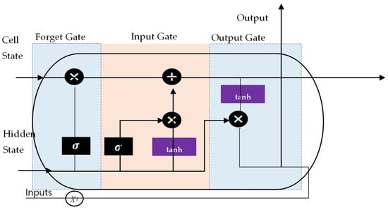
Figure 1.
Architecture of LSTM blocks.
The forget gate eliminates information from the cell state. The ability of LSTM to store or remove information outperforms other neural networks [35]. Information can be carried over multiple time steps and provide for learning of sequential dependency in the input data, making it relevant even for long time series [36]. This gives an advantage to the LSTM when it comes to modeling time series, particularly hydrologic variables, which employ common hyperparameters, such as precipitation, flow or water level, for streamflow prediction, water quality modeling and flood forecasting [37]. Although the training process is longer than other data-driven models, LSTM can yield higher accuracy [38].
2.2. Bat Algorithm
The bat algorithm (see Figure 2) is a swarm intelligence algorithm inspired by the echolocation produced by bats when interacting with their surroundings [23]. The echolocation starts with the emission of short and loud sound waves released by bats to identify their prey, obstacles or resting cracks in the dark. The time-lapse for the emitted sound to bounce back reveals the prey’s distance, direction and speed. All bats use echolocation to measure distance and distinguish between targets and obstacles [39]. The algorithm keeps a record of the bat’s velocity, position, frequency, varying wavelength, loudness and pulse emission. The loudness is measured in the range between Amin and A0, while the pulse emission is logged between 0 and 1, where 0 represents no pulse, and 1 refers to the highest rate of the bat’s emission. The bat algorithm is suitable to handle both continuous and discrete optimization matters. One of the advantages of this algorithm is the ability to reach quick convergence at the initial stage and shift from exploration to exploitation when optimality is near [40].
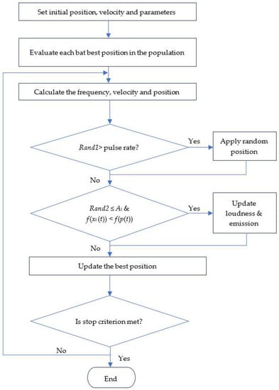
Figure 2.
Bat algorithm flowchart.
The mathematical equations that relate to the velocity and location can be defined as:
where:
is the random vector from a uniform distribution;
is the initial frequency;
is the velocity at iteration;
is location at iteration in a d-dimensional search or solution space.
The loudness and pulse emission rates are represented below:
where:
0 < < 1 and > 0 are constants;
is the constant reducing loudness, and is the constant increasing pulse rate.
2.3. Firefly Algorithm
Bioluminescence refers to the biochemical process that provides the insects’ ability to flicker. The flashing light is visible, particularly at night, to court potential mates and gives a warning signal for potential predators nearby. The emission of the rays can be controlled towards brighter or dimmer light [41].
The firefly algorithm (see Figure 3) is considered a swarm intelligence algorithm that originated from the flickering behaviors of insects. It is a popular algorithm in the swarm intelligence domain [42]. Flashlight without gender distinction is simulated to entice fireflies with less brightness to draw toward the individual. Under this algorithm (see Figure 3), two significant features are considered, mainly brightness and attractiveness. The brightness echoes the firefly’s position and establishes the path of movement. At the same time, the attraction indicates the distance the firefly travels. The algorithm’s goal is to continuously update the brightness and attractiveness status [15].
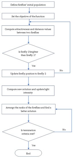
Figure 3.
Firefly algorithm flowchart.
The light brightness will decrease as distance increases. Since the brighter fireflies attract the dimmer ones, the latter will move toward the former position. The brightness indicates the fitness value of the algorithm. The greater the brightness, the better will be the fitness value. If two adjacent fireflies transmit similar brightness, the fireflies will move randomly.
The algorithm is set to adhere to the three following rules [43]:
- (a)
- All fireflies are considered unisex, and therefore, they are attracted to others regardless of their sex;
- (b)
- Attractiveness is based on the brightness of the light. The dimmer one will move towards the brighter one. If brightness is equal, movement will be random;
- (c)
- The brightness is associated with the objective of the function.
When firefly is attracted to , then the new position of the firefly will be computed as follows:
where:
is the new position of the firefly ;
is the original position of the firefly ;
is the attractiveness parameter;
is the absorption coefficient;
is randomization parameter (0 to 1);
r is the distance between two fireflies;
is random number.
2.4. Jaya Algorithm
Jaya algorithm (see Figure 4) is a population-based algorithm that constantly searches for the best solutions and avoids bad ones [29,44]. Two main parameters, the population size and the maximum number of iterations, are used to define the framework of the algorithm [45]. The iteration process will continue to be executed to find a better solution [46] than the current state with the following equation:
where:
is the current state;
is the best solution;
is the worst solution.

Figure 4.
Jaya algorithm.
Figure 4.
Jaya algorithm.

The process will remain until the stopping criteria are met. Jaya algorithm is suitable for controlled and unrestricted optimization [22].
2.5. Rates of Change
Rates of change () is introduced as a new model development method to replace the conventional method of utilizing flow or water level as the prediction model output. The current research on streamflow forecasting concentrates mainly on the prediction of the flow or water level as the output variables of the forecasted value (. The mathematical expression of a forecast flowrate is as follows:
where:
is the forecast flowrate;
is the initial flowrate at the time, t;
is the rate of change.
A rate of change is proposed in this study based on the mathematical relationship as follows:
where:
is the rate of change;
is the flowrate at current time, ;
is the initial flowrate at a previous time interval;
is the current time;
is the last time interval.
By applying the rates of change (, the fluctuation can be controlled to improve the model’s accuracy. For this research, the will be based on 30 min.
2.6. Model Performance Evaluation
In this study, the performance of each model is evaluated based on four types of performance indices. The evaluation includes both the absolute and relative aspects of the errors, such as the root mean square error (RMSE), mean absolute error (MAE), correlation coefficient (R), Nash–Sutcliffe efficiency (NSE) and mean absolute percentage error (MAPE).
2.6.1. Root Mean Square Error, RMSE
RMSE measures the deviations between predicted values and observed values. The variations, also known as the prediction errors, are developed from computation performed over out-of-sample data. RMSE is sensitive to maximum and minimum errors and can better reflect the predicted results. However, it is not sensitive to linear offsets between the observed and simulated values resulting in a low RMSE value [47]. RMSE with a value close to 0 indicates a higher level of prediction accuracy.
where:
are the observed values of the criterion;
are the simulated values of the criterion;
n = sample size.
2.6.2. Mean Absolute Error, MAE
MAE measures the significance of average error in a model with the same criteria [48].
The mathematical representation of MAE is as follows:
where:
are the observed values of the criterion;
are the simulated values of the criterion;
= sample size.
2.6.3. Nash-Sutcliffe Efficiency (NSE)
NSE measures the relative differences between the observed and predicted values. A higher value of NSE indicates the model’s superiority. When NSE is 1, it means a perfect match of the observed and predicted. Otherwise, if NSE is 0, the predicted values are similar to the average of the observed values [49]. The model accuracy can be categorized as very good for 0.75 < NSE ≤ 1, good for 0.65 < NSE ≤ 0.75, satisfactory for 0.50 < NSE ≤ 0.65 or unsatisfactory for NSE ≤ 0.50 [50].
The mathematical representation of NSE is as follows:
where:
Yi is the predicted values of the criterion;
Yt is the measured value of the criterion variable (dependent) variable Y;
is the mean of the measured values of Y;
= sample size.
2.6.4. Mean Absolute Percentage Error (MAPE)
MAPE is an error metric used to measure the accuracy of forecasting values. It denotes the average absolute percentage deviation of each dataset entry between actual and forecast values [51]. As absolute values are applied, the possibility of negative and positive errors canceling each other out can be avoided. The lower the value of MAPE, the better the model will forecast.
where:
is the actual value;
is the forecast value;
= sample size.
2.7. Study Area and Data Description
Malaysia’s climate is hot and with high humidity all year round. The country is exposed to two major monsoon seasons, mainly the north-east monsoon from November to February and the south-west monsoon from May to August. During the north-east monsoon, a significant increase in rainfall occurrence can be detected in the eastern and southern regions of the country. Moreover, the south-west monsoon and inter-monsoon seasons of March to April and September to October can cause intense convective rainfall on the country’s west coast.
Kuala Lumpur is Malaysia’s capital city, as shown in Figure 5. The city is highly urbanized and covers an area of 243 km2 with an estimated population density of 6696 residents per square kilometer [52]. Changes in land use and land cover have been intense since the 1980s due to the economic boom. The city receives an average annual rainfall of 2600 mm and is subjected to flash floods. It is situated in the middle of the Klang River basin with a watershed area of 1288 km2. The Klang River flows through a 120 km distance [53], with 11 major tributaries flowing across Selangor state and Kuala Lumpur [54]. Batu, Gombak, Ampang and upper Klang River at the upper catchment of Kuala Lumpur are the main tributaries of Klang River that contribute significantly to the flow at the downstream point of Masjid Jamek, which is a famous historical site and a tourist attraction.
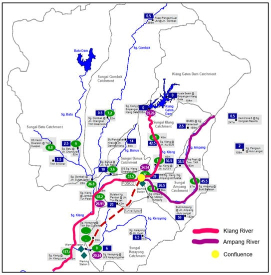
Figure 5.
Map of study location at the Klang River Catchment.
The flash flood occurrence in 1971 that lasted for five days with massive damage of RM36 million prompted the government to develop a comprehensive Kuala Lumpur Flood Mitigation Plan (KLFM) [55]. The Stormwater Management and Road Tunnel (SMART) project built in 2007 is part of the early plan to divert flow from the upper catchment of the Klang River and Ampang River to the Kerayong River downstream [56].
SMART is a mega project to construct a 9.7 km tunnel that combines wet and dry systems [52]. During a major storm, mode 2 is activated when the flow reaches more than 70 m3/s at the confluence of the Klang and Ampang rivers [57]. Moreover, Mode 3 is activated when the flow at the confluence reaches 150 m3/s. Total storage of 3 million3 infrastructure is available to cater for the excess stormwater. During regular days, a total length of 3 km is available for dual-deck motorway use [57].
Study Data
The SMART catchment has an area of 160 km2 equipped with a rain gauge and doppler current meter at 28 hydrological stations. The sensors collect rainfall and flow data and transmit the data to the control center using telemetry. Within the 28 hydrological stations, data from 11 telemetry stations are used for modeling. The rest of the stations are meant for observation only. This study collects historical data of 30 min interval rainfall at the 11 telemetry stations and the flow at the confluence of the Klang River and Ampang River from January 2008 to August 2021. Seventy percent of the historical data from January 2008 to August 2019 are used for training, while the rest are used for testing. Normal flow at the confluence of Ampang and Klang Rivers is generally within the range of 5 to 10 m3/s. However, this flow can increase tremendously above 150 m3/s depending on the intensity of the precipitation.
2.8. Model Development
As shown in Figure 6, the proposed artificial intelligence model is intended to seek the best fit that yields the best results for deployment purposes. Input data for the model consist of historical rainfall data from 11 telemetry stations at the upper catchment of the Klang River basin taken from 1 January 2008 to August 2021 with an interval of 30 min. Moreover, the target data consist of flow data at the confluence between the Ampang–Klang rivers with equal intervals and similar time ranges. The confluence is considered the point of interest in this study as the current flow will determine the mode of operation, as mentioned earlier. Three steps of model development are introduced to pursue the best relationship between historical data and predictors.
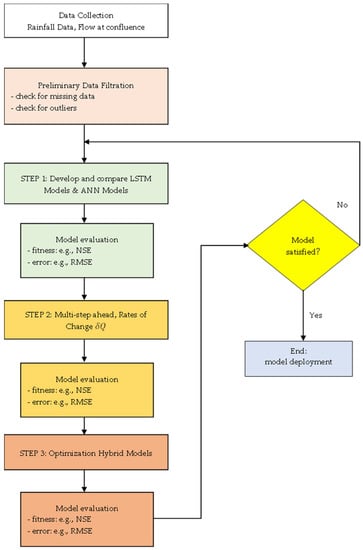
Figure 6.
Model development flowchart.
Step 1 employs the LSTM model as the deep learning framework for streamflow prediction, and ANN is the benchmark model. Several performance indices are performed to compare the models.
Step 2 introduces the novel rates of change method and implements multi-step ahead forecasting to analyze the results better. The models’ performance on fitness and errors are checked.
Step 3 develops the novel optimization method for deep learning using metaheuristics to find the near-optimum weights and biases. Three optimization algorithms were picked for this study: bat algorithm, firefly algorithm and Jaya algorithm. After going through the optimization algorithm, the data are fed into the LSTM model. Performances on fitness and errors are checked. The best model is deployed after the three steps.
3. Results and Discussion
This section unveils the results acquired from the training and testing of various LSTM models. There are three steps involved (refer to Figure 6). For Step 1, numerous LSTM and ANN models are employed to perform streamflow prediction. The performance is evaluated for the goodness of fit by executing several measures listed in Section 2.6. Table 1 lists the best model results of the LSTM and ANN. Figure 7 and Figure 8 show the graphs of observed flow vs. forecast flow for the ANN model and LSTM model, respectively.

Table 1.
Best LSTM and ANN models for prediction.
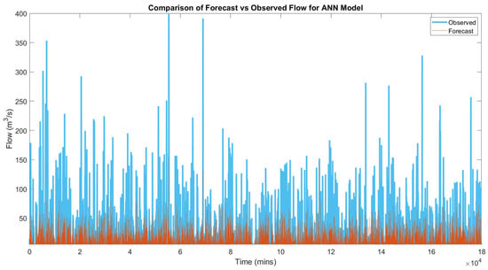
Figure 7.
Graph of ANN model observed flow vs. simulated flow.
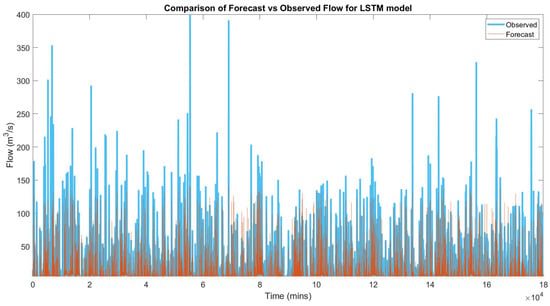
Figure 8.
Graph of LSTM observed flow vs. simulated flow.
Step 2 introduces rates of change and executes multi-step ahead forecasting to facilitate the flood mitigation operation better. LSTM models are performed on multiple conditions, mainly simulation, 30 min ahead forecasting, 1 h ahead forecasting and rates of change . Table 2 lists the performance of this exercise.
Table 2.
LSTM forecasting models.
Step 3 develops several new hybrids of artificial intelligence. Three metaheuristic frameworks are selected for execution with the deep learning LSTM models: the bat algorithm, firefly algorithm and Jaya algorithm. Table 3 shows the streamflow prediction performance models for the hybrid model of the bat algorithm and LSTM. The parameters set for these models consist of maximum iteration = 40, alpha = 0.95, gamma = 0.95, bat numbers = 4, bat minimum frequency = 0, bat maximum frequency = 1 and maximum epochs = 500.
Table 3.
Performance of LSTM with bat algorithm models for streamflow.
Table 4 displays the performance of the LSTM model after integration with the firefly algorithm. The parameters set for these models consist of maximum iteration = 40, alpha = 0.95, betta = 1, gamma = 0.95, firefly numbers = 4 and maximum epochs = 500.
Table 4.
Performance of LSTM with firefly algorithm models for streamflow.
Table 5 shows the performance of the LSTM model with the Jaya algorithm. The parameters set for these models consist of maximum iteration = 30, population = 5 and maximum epochs = 500.
Table 5.
Performance of LSTM with Jaya algorithm models for streamflow simulation.
Figure 9 displays graphs of observed vs. forecast flow based on simulation, 30 min ahead forecasting, 1 h ahead forecasting and rates of change model.
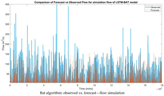

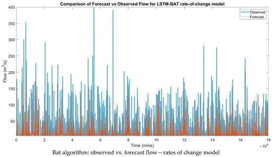
Figure 9.
Graphs of optimization-LSTM hybrid models.
A further check is performed on the hybrid optimization models to determine the MAPE, MAE and maximum error values for the flows equal to or greater than 150 m3/s. This ensures the accuracy of forecasting high flow values, which is important in a flood mitigation operation.
3.1. Performance of Step 1
In Step 1, the LSTM and ANN algorithms were developed and compared. It was found that LSTM performed much better than ANN. Several literature reviews also supported this by identifying the LSTM as the best deep learning model for time series data due to its ability to keep selective memory. LSTM algorithm could also filter the hydrological noise and retrieve the intrinsic characteristics of the hydrological series for simulation and future forecasting purposes.
Table 1 indicated that the ANN model had a regression of 0.4520, MSE 78.4215, MAE 3.7135 m3/s, NSE 0.1994 and RMSE 8.8556 m3/s. Furthermore, the best LSTM had regression 0.9055, MSE 17,8532, MAE 1.4365 m3/s, NSE 0.8190 and RMSE 5.3695 m3/s. Generally, it had shown a double improvement in overall results.
3.2. Performance of Step 2
Step 2 introduced rates of change as an innovative approach to the model development. In addition, multi-step ahead forecasting was performed as a requirement for flood mitigation operations. Table 2 revealed that the worst result was acquired for the 1 h ahead forecasting, where the regression value for training was the lowest at 0.8849. However, it had a better regression value for testing when compared to simulation. This trend was applicable to MSE and MAE for having the worst values. The NSE value also turned out to be the worst. Considering the longer forecasting time, the results of this study were still regarded as logical and satisfactory. The longer the forecasting time, the more uncertainties and missing information would appear.
The output from 30 min ahead forecasting turned out to be quite good as it had a regression training value of 0.9470, and the regression value for testing was not far off, which was 0.9476. The MSE and MAE values were low, which was good, with acceptable values for NSE and RMSE.
However, the best performance of the model was discovered with the novel method when applying rates of change as the target values. The regression value for training was the highest, 0.9545, while the error values were the lowest. The NSE value was the highest, 0.9090, while the RMSE was the lowest at 2.9958 m3/s. The model was the most superior among the four models tested.
The study did not seek an experiment of more than 1 h forecasting as the lag time determined was 30 min for this catchment. The results would deteriorate further as the time of forecasting increased.
3.3. Performance of Step 3
Step 3 was one of the main contributions of this study. Current metaheuristics studies mainly concentrate on developing a hybrid model with ANN or primary neural networks. Therefore, this study initiated the hybrid models for the deep learning algorithm, mainly the LSTM. Three metaheuristic frameworks, the bat algorithm, firefly algorithm and Jaya algorithm, were selected for this study. The bat algorithm and firefly algorithm belonged to swarm intelligence algorithms. They required trials on nature-based characteristics to find the optimum yield. Jaya algorithm, on the other hand, was designed based on searching for the best solutions. The effort to introduce numerous hybrid optimization algorithms was intended to further enhance the model performance results from steps 1 and 2.
Table 3, Table 4 and Table 5 represent each of the selected optimization algorithms. From the three tables, it was determined that all the hybrid models produced better results. However, the best model identified was the bat-LSTM hybrid algorithm where the model yielded R.train 0.9757, R.test 0.9046, MSE.train 4.7187, MSE.test 19.8966, MAE.train 0.4672 m3/s, MAE.test 0.8565 m3/s, NSE 0.9514 and RMSE 2.1723 m3/s.
The results also proved that the choice of metaheuristic algorithms did not significantly impact the performance. The performance inclination is still the same as the LSTM-only model in step 2, where 30 min ahead of forecasting yielded the best results. As the time of forecasting increased, the results deteriorated accordingly. models consistently yielded the best results by keeping the error values to a minimum.
This process was then followed by the plotting of a peak-to-peak flow graph between the observed and the forecast values. Figure 9 indicated that the best graph with the highest accuracy was the models.
A further experiment was performed to seek high flow performance for each hybrid model in terms of MAPE, MAE and maximum error. This study concentrates on the flows equal to or greater than 150 m3/s, which was the high flow indicator to initiate modes 3 and 4 in the SMART control center’s standard operating procedure. The results are tabulated in Table 6. From the results, it could be seen that models again outperformed the rest with the smallest error values, where the bat and Jaya algorithms yielded the best with MAPE 6.33%, MAE 12.2865 m3/s and maximum error 97.70% for bat-LSTM algorithm while MAPE 6.22%, MAE 12.6687 m3/s and maximum error 97.70% for Jaya-LSTM algorithm. The maximum error values could be ignored in this case as they could not represent the overall performance of the models.
Table 6.
Performance of LSTM-optimization algorithm models for streamflow forecasting.
4. Conclusions
The effectiveness of flood management and disaster preparedness is in tandem with the ability to accurately forecast the immediate condition of streamflow in the catchment area. This study intended to develop the best deep learning model for the SMART control center in managing the river flow through streamflow forecasting. The aim was to create a novel approach in using rates of change for model development and introduce new metaheuristic algorithms with LSTM hybrid models to enhance the performance results.
This study employed LSTM models to develop and train historical data at the Ampang River and Klang River. The task is to forecast river streamflow with simulation, 30 min ahead, 1 h ahead and rates-of-change models. In order to ascertain the best performance that can be achieved, three steps of the improvement process were introduced.
Step 1 is where the comparison of ANN and LSTM models is performed. The best results come from the LSTM model with regression 0.9055, MSE 17,8532, MAE 1.4365 m3/s, NSE 0.8190 and RMSE 5.3695 m3/s. ANN yielded weaker results, and therefore LSTM model is the center of this research.
Step 2 introduces rates of change and performs multi-step ahead streamflow forecasting. The best result comes from the model with performance values of R (training) = 0.9545, R (testing) = 0.9214, MSE (training) = 8.9746, MSE (testing) = 15.6981, MAE (training) = 0.5434 m3/s, MAE (testing) = 0.8108 m3/s, NSE = 0.9090 and RMSE = 2.9958 m3/s. The finding reveals that a shorter forecasting time yields better performance results. The second finding shows that applying new rate changes in model development has significantly improved the model results.
The last step of the experiment is to introduce new hybrid models between optimization and LSTM algorithms. The bat algorithm, firefly algorithm and Jaya algorithm were selected for this study. From the results, all hybrid models demonstrate better outcomes. Therefore, the third finding shows that metaheuristic algorithms play a role in model improvement. Under this study, it is also noticeable that the selection of an optimization algorithm does not significantly affect performance.
model for the bat algorithm with LSTM hybrid model yielded the best results with R (training) = 0.9757, R (testing) = 0.9046, MSE (training) = 4.7187, MSE (testing) = 19.8966, MAE (training) = 0.4672 m3/s, MAE (testing) = 0.8565 m3/s, NSE = 0.9514 and RMSE = 2.1723 m3/s.
Findings from this study are beneficial to improving the deep learning process so that the performance can yield better results with higher precision. This knowledge also helps elevate a new approach to flood mitigation operations. This study is significant as it has presented several new steps to improve the learning process leading to a better relationship between the input and output data. The current study is limited to a small catchment area and several optimization models. The results may differ for bigger catchments and with more optimization models. In order to further improve the experiment, it is suggested to try reinforcement learning for future studies.
Author Contributions
All authors contributed to the study and design. Material preparation, data collection, investigation, resources, data curation and analysis were performed by W.Y.T.; S.H.L. contributed to conceptualization, methodology, software teaching and supervision; F.Y.T. contributed to supervision; D.J.A. contributed to resources and funding acquisition; K.P. contributed to the software development; and A.E.-S. contributed to project management, visualization and supervision. The first draft of the manuscript was written by W.Y.T. and all authors commented on previous versions of the manuscript. All authors have read and agreed to the published version of the manuscript.
Funding
This research did not receive any specific grant from funding agencies in the public, commercial, or not-for-profit sectors.
Institutional Review Board Statement
Not applicable.
Informed Consent Statement
Not applicable.
Data Availability Statement
The data is available but subject to approval from the original data owner first.
Conflicts of Interest
The authors declare no conflict of interest.
References
- Ahmed, A.M.; Deo, R.C.; Feng, Q.; Ghahramani, A.; Raj, N.; Yin, Z.; Yang, L. Deep learning hybrid model with Boruta-Random forest optimiser algorithm for streamflow forecasting with climate mode indices, rainfall, and periodicity. J. Hydrol. 2021, 599, 126350. [Google Scholar] [CrossRef]
- Reis, G.B.; da Silva, D.D.; Filho, E.I.F.; Moreira, M.C.; Veloso, G.V.; Fraga, M.D.S.; Pinheiro, S.A.R. Effect of environmental covariable selection in the hydrological modeling using machine learning models to predict daily streamflow. J. Environ. Manag. 2021, 290, 112625. [Google Scholar] [CrossRef] [PubMed]
- Ni, L.; Wang, D.; Wu, J.; Wang, Y.; Tao, Y.; Zhang, J.; Liu, J. Streamflow forecasting using extreme gradient boosting model coupled with Gaussian mixture model. J. Hydrol. 2020, 586, 124901. [Google Scholar] [CrossRef]
- Marechal, D. A Soil-Based Approach to Rainfall-Runoff Modelling in Ungauged Catchments for England and Wales. Ph.D. Thesis, Cranfield University, Cranfield, UK, 2004; p. 145. [Google Scholar]
- Kao, I.-F.; Liou, J.-Y.; Lee, M.-H.; Chang, F.-J. Fusing stacked autoencoder and long short-term memory for regional multistep-ahead flood inundation forecasts. J. Hydrol. 2021, 598, 126371. [Google Scholar] [CrossRef]
- Lin, Y.; Wang, D.; Wang, G.; Qiu, J.; Long, K.; Du, Y.; Xie, H.; Wei, Z.; Shangguan, W.; Dai, Y. A hybrid deep learning algorithm and its application to streamflow prediction. J. Hydrol. 2021, 601, 126636. [Google Scholar] [CrossRef]
- Xiang, Z.; Demir, I. Distributed long-term hourly streamflow predictions using deep learning—A case study for State of Iowa. Environ. Model. Softw. 2020, 131, 104761. [Google Scholar] [CrossRef]
- Granata, F.; Di Nunno, F.; de Marinis, G. Stacked machine learning algorithms and bidirectional long short-term memory networks for multi-step ahead streamflow forecasting: A comparative study. J. Hydrol. 2022, 613, 128431. [Google Scholar] [CrossRef]
- Elbeltagi, A.; Di Nunno, F.; Kushwaha, N.L.; de Marinis, G.; Granata, F. River flow rate prediction in the Des Moines watershed (Iowa, USA): A machine learning approach. Stoch. Environ. Res. Risk Assess. 2022, 36, 3835–3855. [Google Scholar] [CrossRef]
- Peng, H.; Xiao, W.; Han, Y.; Jiang, A.; Xu, Z.; Li, M.; Wu, Z. Multi-strategy firefly algorithm with selective ensemble for complex engineering optimization problems. Appl. Soft Comput. 2022, 120, 108634. [Google Scholar] [CrossRef]
- Karimi-Mamaghan, M.; Mohammadi, M.; Meyer, P.; Karimi-Mamaghan, A.M.; Talbi, E.-G. Machine learning at the service of meta-heuristics for solving combinatorial optimization problems: A state-of-the-art. Eur. J. Oper. Res. 2022, 296, 393–422. [Google Scholar] [CrossRef]
- Khosravi, K.; Golkarian, A.; Tiefenbacher, J.P. Using Optimized Deep Learning to Predict Daily Streamflow: A Comparison to Common Machine Learning Algorithms. Water Resour. Manag. 2022, 36, 699–716. [Google Scholar] [CrossRef]
- Gambella, C.; Ghaddar, B.; Naoum-Sawaya, J. Optimization problems for machine learning: A survey. Eur. J. Oper. Res. 2021, 290, 807–828. [Google Scholar] [CrossRef]
- Bayındır, Y.; Yolcu, O.C.; Temel, F.A.; Turan, N.G. Evaluation of a cascade artificial neural network for modeling and optimization of process parameters in co-composting of cattle manure and municipal solid waste. J. Environ. Manag. 2022, 318, 115496. [Google Scholar] [CrossRef] [PubMed]
- Zhang, W.; Gu, X.; Tang, L.; Yin, Y.; Liu, D.; Zhang, Y. Application of machine learning, deep learning and optimization algorithms in geoengineering and geoscience: Comprehensive review and future challenge. Gondwana Res. 2022, 109, 1–17. [Google Scholar] [CrossRef]
- Ibrahim, K.S.M.H.; Huang, Y.F.; Ahmed, A.N.; Koo, C.H.; El-Shafie, A. A review of the hybrid artificial intelligence and optimization modelling of hydrological streamflow forecasting. Alex. Eng. J. 2021, 61, 279–303. [Google Scholar] [CrossRef]
- Horne, A.; Szemis, J.M.; Kaur, S.; Webb, J.A.; Stewardson, M.J.; Costa, A.; Boland, N. Optimization tools for environmental water decisions: A review of strengths, weaknesses, and opportunities to improve adoption. Environ. Model. Softw. 2016, 84, 326–338. [Google Scholar] [CrossRef]
- Song, H.; Triguero, I.; Özcan, E. A review on the self and dual interactions between machine learning and optimisation. Prog. Artif. Intell. 2019, 8, 143–165. [Google Scholar] [CrossRef]
- Li, H.; Song, B.; Tang, X.; Xie, Y.; Zhou, X. A multi-objective bat algorithm with a novel competitive mechanism and its application in controller tuning. Eng. Appl. Artif. Intell. 2021, 106, 104453. [Google Scholar] [CrossRef]
- Ben, U.C.; Akpan, A.E.; Urang, J.G.; Akaerue, E.I.; Obianwu, V.I. Novel methodology for the geophysical interpretation of magnetic anomalies due to simple geometrical bodies using social spider optimization (SSO) algorithm. Heliyon 2022, 8, e09027. [Google Scholar] [CrossRef]
- Ahmed, A.N.; Van Lam, T.; Hung, N.D.; Van Thieu, N.; Kisi, O.; El-Shafie, A. A comprehensive comparison of recent developed meta-heuristic algorithms for streamflow time series forecasting problem. Appl. Soft Comput. 2021, 105, 107282. [Google Scholar] [CrossRef]
- Rao, R.V. Jaya: A simple and new optimization algorithm for solving constrained and unconstrained optimization problems. Int. J. Ind. Eng. Comput. 2016, 7, 19–34. [Google Scholar] [CrossRef]
- Malek, M.R.A.; Aziz, N.A.A.; Alelyani, S.; Mohana, M.; Baharudin, F.N.A.; Ibrahim, Z. Comfort and energy consumption optimization in smart homes using bat algorithm with inertia weight. J. Build. Eng. 2022, 47, 103848. [Google Scholar] [CrossRef]
- Lu, P.; Ye, L.; Zhao, Y.; Dai, B.; Pei, M.; Tang, Y. Review of meta-heuristic algorithms for wind power prediction: Methodologies, applications and challenges. Appl. Energy 2021, 301, 117446. [Google Scholar] [CrossRef]
- Calvet, L.; de Armas, J.; Masip, D.; Juan, A.A. Learnheuristics: Hybridizing metaheuristics with machine learning for optimization with dynamic inputs. Open Math. 2017, 15, 261–280. [Google Scholar] [CrossRef]
- Yang, X.-S. Multiobjective firefly algorithm for continuous optimization. Eng. Comput. 2012, 29, 175–184. [Google Scholar] [CrossRef]
- Ding, Z.; Hou, R.; Xia, Y. Structural damage identification considering uncertainties based on a Jaya algorithm with a local pattern search strategy and L0.5 sparse regularization. Eng. Struct. 2022, 261, 114312. [Google Scholar] [CrossRef]
- Kang, F.; Wu, Y.; Li, J.; Li, H. Dynamic parameter inverse analysis of concrete dams based on Jaya algorithm with Gaussian processes surrogate model. Adv. Eng. Inform. 2021, 49, 101348. [Google Scholar] [CrossRef]
- Degertekin, S.; Bayar, G.Y.; Lamberti, L. Parameter free Jaya algorithm for truss sizing-layout optimization under natural frequency constraints. Comput. Struct. 2020, 245, 106461. [Google Scholar] [CrossRef]
- Xu, Y.; Hu, C.; Wu, Q.; Jian, S.; Li, Z.; Chen, Y.; Zhang, G.; Zhang, Z.; Wang, S. Research on particle swarm optimization in LSTM neural networks for rainfall-runoff simulation. J. Hydrol. 2022, 608, 127553. [Google Scholar] [CrossRef]
- Alizadeh, B.; Bafti, A.G.; Kamangir, H.; Zhang, Y.; Wright, D.B.; Franz, K.J. A novel attention-based LSTM cell post-processor coupled with bayesian optimization for streamflow prediction. J. Hydrol. 2021, 601, 126526. [Google Scholar] [CrossRef]
- Johny, K.; Pai, M.L.; Adarsh, S. A multivariate EMD-LSTM model aided with Time Dependent Intrinsic Cross-Correlation for monthly rainfall prediction. Appl. Soft Comput. 2022, 123, 108941. [Google Scholar] [CrossRef]
- Dikshit, A.; Pradhan, B.; Huete, A. An improved SPEI drought forecasting approach using the long short-term memory neural network. J. Environ. Manag. 2021, 283, 111979. [Google Scholar] [CrossRef] [PubMed]
- Ishii, K.; Sato, M.; Ochiai, S. Prediction of leachate quantity and quality from a landfill site by the long short-term memory model. J. Environ. Manag. 2022, 310, 114733. [Google Scholar] [CrossRef] [PubMed]
- Ni, L.; Wang, D.; Singh, V.P.; Wu, J.; Wang, Y.; Tao, Y.; Zhang, J. Streamflow and rainfall forecasting by two long short-term memory-based models. J. Hydrol. 2020, 583, 124296. [Google Scholar] [CrossRef]
- Anshuman, A.; Eldho, T. Entity aware sequence to sequence learning using LSTMs for estimation of groundwater contamination release history and transport parameters. J. Hydrol. 2022, 608, 127662. [Google Scholar] [CrossRef]
- Sadler, J.M.; Appling, A.P.; Read, J.S.; Oliver, S.K.; Jia, X.; Zwart, J.A.; Kumar, V. Multi-Task Deep Learning of Daily Streamflow and Water Temperature. Water Resour. Res. 2022, 58, e2021WR030138. [Google Scholar] [CrossRef]
- Han, H.; Morrison, R.R. Improved runoff forecasting performance through error predictions using a deep-learning approach. J. Hydrol. 2022, 608, 127653. [Google Scholar] [CrossRef]
- Yang, X.-S.; He, X. Bat algorithm: Literature review and applications. Int. J. Bio-Inspired Comput. 2013, 5, 141–149. [Google Scholar] [CrossRef]
- Fister, I.; Yang, X.-S.; Fong, S.; Zhuang, Y. Bat algorithm: Recent advances. In Proceedings of the 2014 IEEE 15th International symposium on computational intelligence and informatics (CINTI), Budapest, Hungary, 19–21 November 2014; pp. 163–167. [Google Scholar] [CrossRef]
- Kumar, V.; Kumar, D. A Systematic Review on Firefly Algorithm: Past, Present, and Future. Arch. Comput. Methods Eng. 2020, 28, 3269–3291. [Google Scholar] [CrossRef]
- Li, J.; Wei, X.; Li, B.; Zeng, Z. A survey on firefly algorithms. Neurocomputing 2022, 500, 662–678. [Google Scholar] [CrossRef]
- Yang, X. Firefly Algorithms for Multimodal Optimization. In International Symposium on Stochastic Algorithms; Springer: Berlin/Heidelberg, Germany, 2009; Volume 5792, pp. 169–178. [Google Scholar]
- Abu Zitar, R.; Al-Betar, M.A.; Awadallah, M.A.; Abu Doush, I.; Assaleh, K. An Intensive and Comprehensive Overview of JAYA Algorithm, Its Versions and Applications. Arch. Comput. Methods Eng. 2021, 29, 763–792. [Google Scholar] [CrossRef] [PubMed]
- Aslay, S.E.; Dede, T. 3D cost optimization of 3 story RC constructional building using Jaya algorithm. Structures 2022, 40, 803–811. [Google Scholar] [CrossRef]
- Zhao, F.; Zhang, H.; Wang, L.; Ma, R.; Xu, T.; Zhu, N. A surrogate-assisted Jaya algorithm based on optimal directional guidance and historical learning mechanism. Eng. Appl. Artif. Intell. 2022, 111, 104775. [Google Scholar] [CrossRef]
- Jackson, E.K.; Roberts, W.; Nelsen, B.; Williams, G.P.; Nelson, E.J.; Ames, D.P. Introductory overview: Error metrics for hydrologic modelling—A review of common practices and an open source library to facilitate use and adoption. Environ. Model. Softw. 2019, 119, 32–48. [Google Scholar] [CrossRef]
- Althoff, D.; Rodrigues, L.N. Goodness-of-fit criteria for hydrological models: Model calibration and performance assessment. J. Hydrol. 2021, 600, 126674. [Google Scholar] [CrossRef]
- Feng, Z.-K.; Shi, P.-F.; Yang, T.; Niu, W.-J.; Zhou, J.-Z.; Cheng, C.-T. Parallel cooperation search algorithm and artificial intelligence method for streamflow time series forecasting. J. Hydrol. 2022, 606, 127434. [Google Scholar] [CrossRef]
- Kim, T.; Yang, T.; Gao, S.; Zhang, L.; Ding, Z.; Wen, X.; Gourley, J.J.; Hong, Y. Can artificial intelligence and data-driven machine learning models match or even replace process-driven hydrologic models for streamflow simulation? A case study of four watersheds with different hydro-climatic regions across the CONUS. J. Hydrol. 2021, 598, 126423. [Google Scholar] [CrossRef]
- Ding, Y.; Zhu, Y.; Feng, J.; Zhang, P.; Cheng, Z. Interpretable spatio-temporal attention LSTM model for flood forecasting. Neurocomputing 2020, 403, 348–359. [Google Scholar] [CrossRef]
- Mohtar, W.H.M.W.; Abdullah, J.; Maulud, K.N.A.; Muhammad, N.S. Urban flash flood index based on historical rainfall events. Sustain. Cities Soc. 2020, 56, 102088. [Google Scholar] [CrossRef]
- Zabidi, H.; De Freitas, M.H. Re-evaluation of rock core logging for the prediction of preferred orientations of karst in the Kuala Lumpur Limestone Formation. Eng. Geol. 2011, 117, 159–169. [Google Scholar] [CrossRef]
- Othman, F.; Alaaeldin, M.; Seyam, M.; Ahmed, A.N.; Teo, F.Y.; Fai, C.M.; Afan, H.A.; Sherif, M.; Sefelnasr, A.; El-Shafie, A. Efficient river water quality index prediction considering minimal number of inputs variables. Eng. Appl. Comput. Fluid Mech. 2020, 14, 751–763. [Google Scholar] [CrossRef]
- Kim-Soon, N.; Isah, N.; Ali, M.B.; Bin Ahmad, A.R. Relationships Between Stormwater Management and Road Tunnel Maintenance Works, Flooding and Traffic Flow. Adv. Sci. Lett. 2016, 22, 1845–1848. [Google Scholar] [CrossRef]
- Bell, V.; Rehan, B.; Hasan-Basri, B.; Houghton-Carr, H.; Miller, J.; Reynard, N.; Sayers, P.; Stewart, E.; Toriman, M.E.; Yusuf, B.; et al. Flood Impacts across Scales: Towards an integrated multi-scale approach for Malaysia. In Proceedings of the 4th European Conference on Flood Risk Management (FLOODrisk2020), Online, 22–24 June 2021. [Google Scholar] [CrossRef]
- Alrabie, N.A.; Mohamat-Yusuff, F.; Rohasliney, H.; Zulkeflee, Z.; Amal, M.N.A.; Arshad, A.; Zulkifli, S.Z.; Wijaya, A.R.; Masood, N.; Sani, M.S.A. Preliminary Evaluation of Heavy Metal Contamination and Source Identification in Kuala Lumpur SMART Stormwater Pond Sediments Using Pb Isotopic Signature. Sustainability 2021, 13, 9020. [Google Scholar] [CrossRef]


Publisher’s Note: MDPI stays neutral with regard to jurisdictional claims in published maps and institutional affiliations. |
© 2022 by the authors. Licensee MDPI, Basel, Switzerland. This article is an open access article distributed under the terms and conditions of the Creative Commons Attribution (CC BY) license (https://creativecommons.org/licenses/by/4.0/).