
Crack Location and Degree Detection Method Based on YOLOX Model


Abstract
:1. Introduction
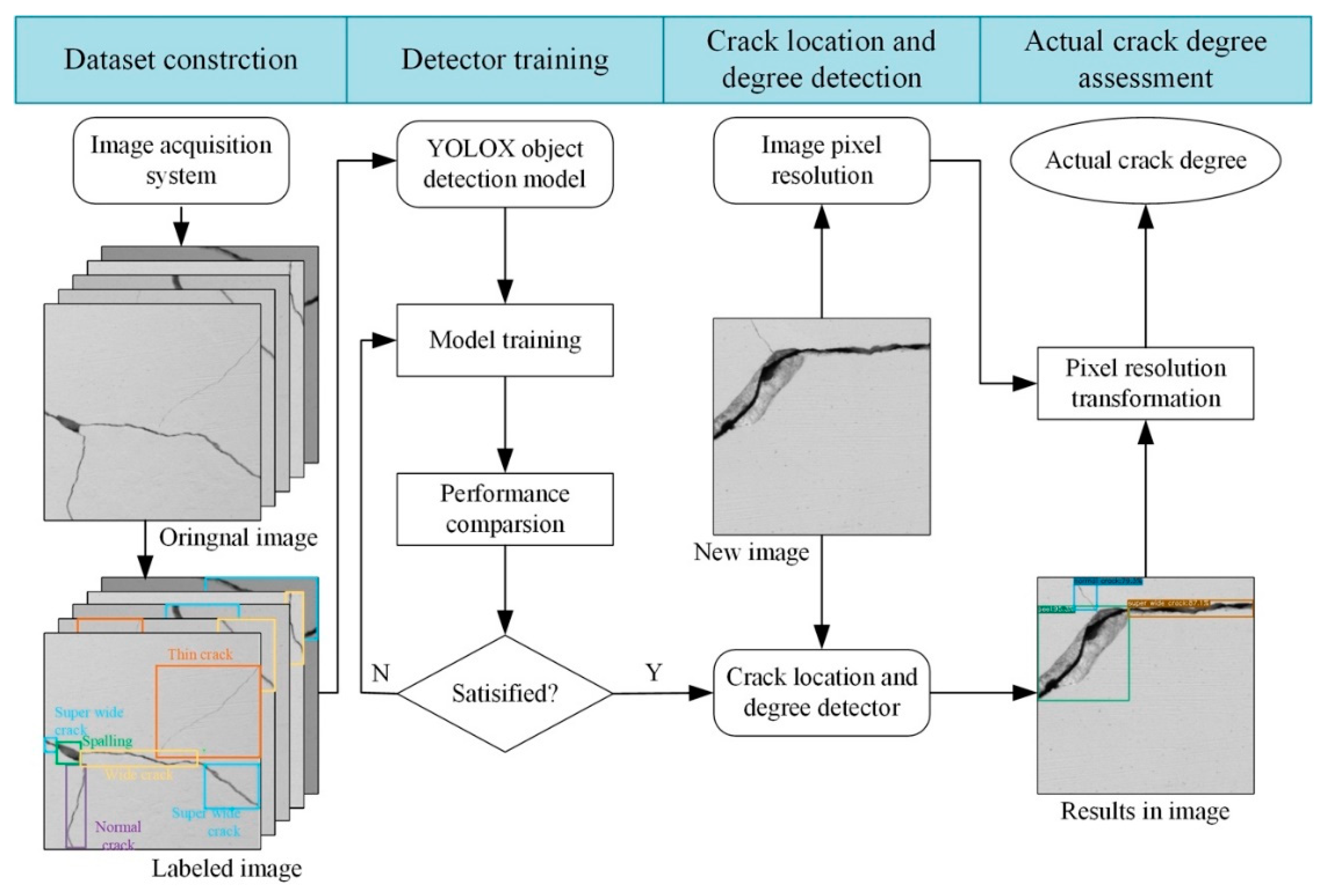
2. Methodology
2.1. The Detection Principle of the Proposed Detector
2.1.1. Input Part
2.1.2. Backbone Network
2.1.3. Neck Network
2.1.4. Prediction Part
2.1.5. The Loss Function of YOLOX
2.2. The Transformation of Crack Degree
3. Dataset Construction
3.1. Image Acquisition System
3.2. Establish Image Dataset with Labels
4. Experimental Results and Analysis
4.1. Model Evaluation Metrics
4.1.1. AP and mAP
4.1.2. Detection Speed and Inference Time
4.2. Training Setting
4.3. Training Results and Analysis
4.4. Test Results and Discussion
4.5. Crack Degree Transformation Test and Results
5. Conclusions and Future Work
Author Contributions
Funding
Institutional Review Board Statement
Informed Consent Statement
Data Availability Statement
Acknowledgments
Conflicts of Interest
References
- Jang, K.; An, Y.-K. Multiple crack evaluation on concrete using a line laser thermography scanning system. Smart Struct. Syst. 2018, 22, 201–207. [Google Scholar] [CrossRef]
- Kim, H.; Lee, J.; Ahn, E.; Cho, S.; Shin, M.; Sim, S.-H. Concrete crack identification using a UAV incorporating hybrid image processing. Sensors 2017, 17, 2052. [Google Scholar] [CrossRef] [PubMed] [Green Version]
- Kim, B.; Yuvaraj, N.; Sri, K.R.; Arun, R. Surface crack detection using deep learning with shallow CNN architecture for enhanced computation. Neural Comput. Appl. 2021, 33, 9289–9305. [Google Scholar] [CrossRef]
- Zhang, H.; Li, J.; Kang, F.; Zhang, J. Monitoring and evaluation of the repair quality of concrete cracks using piezoelectric smart aggregates. Constr. Build. Mater. 2022, 317, 125775. [Google Scholar] [CrossRef]
- Liu, Y.; Cho, S.; Spencer, B.F.; Fan, J. Automated assessment of cracks on concrete surfaces using adaptive digital image processing. Smart Struct. Syst. 2014, 14, 719–741. [Google Scholar] [CrossRef]
- Li, G.; Li, X.; Zhou, J.; Liu, D.; Ren, W. Pixel-level bridge crack detection using a deep fusion about recurrent residual convolution and context encoder network. Measurement 2021, 176, 109171. [Google Scholar] [CrossRef]
- Savino, P.; Tondolo, F. Automated classification of civil structure defects based on convolutional neural network. Front. Struct. Civ. Eng. 2021, 15, 305–317. [Google Scholar] [CrossRef]
- Jahanshahi, M.R.; Masri, S.F.; Sukhatme, G.S. Multi-image stitching and scene reconstruction for evaluating defect evolution in structures. Struct. Health Monit. 2011, 10, 643–657. [Google Scholar] [CrossRef] [Green Version]
- Yang, C.; Chen, J.; Li, Z.; Huang, Y. Structural crack detection and recognition based on deep learning. Appl. Sci. 2021, 11, 2868. [Google Scholar] [CrossRef]
- Jahanshahi, M.R.; Kelly, J.S.; Masri, S.F.; Sukhatme, G.S. A survey and evaluation of promising approaches for automatic image-based defect detection of bridge structures. Struct. Infrastruct. Eng. 2009, 5, 455–486. [Google Scholar] [CrossRef]
- Wang, W.; Hu, W.; Wang, W.; Xu, X.; Wang, M.; Shi, Y.; Qiu, S.; Tutumluer, E. Automated crack severity level detection and classification for ballastless track slab using deep convolutional neural network. Autom. Constr. 2021, 124, 103484. [Google Scholar] [CrossRef]
- Koch, C.; Georgieva, K.; Kasireddy, V.; Akinci, B.; Fieguth, P. A review on computer vision based defect detection and condition assessment of concrete and asphalt civil infrastructure. Adv. Eng. Inform. 2015, 29, 196–210. [Google Scholar] [CrossRef] [Green Version]
- Li, B.; Wang, K.C.P.; Zhang, A.; Yang, E.; Wang, G. Automatic classification of pavement crack using deep convolutional neural network. Int. J. Pavement Eng. 2018, 21, 457–463. [Google Scholar] [CrossRef]
- Mei, Q.; Gül, M.; Azim, M.R. Densely connected deep neural network considering connectivity of pixels for automatic crack detection. Autom. Constr. 2020, 110, 103018. [Google Scholar] [CrossRef]
- Zheng, M.; Lei, Z.; Zhang, K. Intelligent detection of building cracks based on deep learning. Image Vis. Comput. 2020, 103, 03987. [Google Scholar] [CrossRef]
- Bae, H.; Jang, K.; An, Y.-K. Deep super resolution crack network (SrcNet) for improving computer vision–based automated crack detectability in in situ bridges. Struct. Health Monit. 2021, 20, 1428–1442. [Google Scholar] [CrossRef]
- Saleem, M.R.; Park, J.-W.; Lee, J.-H.; Jung, H.-J.; Sarwar, M.Z. Instant bridge visual inspection using an unmanned aerial vehicle by image capturing and geo-tagging system and deep convolutional neural network. Struct. Health Monit. 2020, 20, 1760–1777. [Google Scholar] [CrossRef]
- Xu, Y.; Li, D.; Xie, Q.; Wu, Q.; Wang, J. Automatic defect detection and segmentation of tunnel surface using modified Mask R-CNN. Measurement 2021, 178, 109316. [Google Scholar] [CrossRef]
- Huang, H.-W.; Li, Q.-T.; Zhang, D.-M. Deep learning based image recognition for crack and leakage defects of metro shield tunnel. Tunn. Undergr. Space Technol. 2018, 77, 166–176. [Google Scholar] [CrossRef]
- Tang, J.; Mao, Y.; Wang, J.; Wang, L. Multi-task enhanced dam crack image detection based on Faster R-CNN. In Proceedings of the IEEE 4th International Conference on Image, Vision and Computing, Xiamen, China, 5–7 July 2019; pp. 336–340. [Google Scholar] [CrossRef]
- Zhang, L.; Yang, F.; Zhang, Y.D.; Zhu, Y.J. Road crack detection using deep convolutional neural network. In Proceedings of the IEEE International Conference on Image Processin, Phoenix, AZ, USA, 25–28 September 2016; pp. 3708–3712. [Google Scholar] [CrossRef]
- Wang, B.; Zhao, W.; Gao, P.; Zhang, Y.; Wang, Z. Crack damage detection method via multiple visual features and efficient multi-task learning model. Sensors 2018, 18, 1796. [Google Scholar] [CrossRef] [Green Version]
- Cha, Y.-J.; Choi, W.; Büyüköztürk, O. Deep learning-based crack damage detection using convolutional neural networks. Comput. Aided Civ. Infrastruct. Eng. 2017, 32, 361–378. [Google Scholar] [CrossRef]
- Chen, F.-C.; Jahanshahi, M.R. NB-CNN: Deep learning-based crack detection using convolutional neural network and naïve bayes data fusion. IEEE Trans. Ind. Electron. 2018, 65, 4392–4400. [Google Scholar] [CrossRef]
- Gopalakrishnan, K.; Khaitan, S.K.; Choudhary, A.; Agrawal, A. Deep convolutional neural networks with transfer learning for computer vision-based data-driven pavement distress detection. Constr. Build. Mater. 2017, 157, 322–330. [Google Scholar] [CrossRef]
- Zhang, A.; Wang, K.C.P.; Li, B.; Yang, E.; Dai, X.; Peng, Y.; Fei, Y.; Liu, Y.; Li, J.Q.; Chen, C. Automated pixel-level pavement crack detection on 3D asphalt surfaces using a deep-learning network. Comput. Aided Civ. Infrastruct. Eng. 2017, 32, 805–819. [Google Scholar] [CrossRef]
- Fan, Z.; Wu, Y.; Lu, J.; Li, W. Automatic pavement crack detection based on structured prediction with the convolutional neural network. arXiv 2018, arXiv:1802.02208. [Google Scholar]
- Kim, I.H.; Jeon, H.; Baek, S.C.; Hong, W.H.; Jung, H.J. Application of crack identification techniques for an aging concrete bridge inspection using an unmanned aerial vehicle. Sensors 2018, 18, 1881. [Google Scholar] [CrossRef] [Green Version]
- Dorafshan, S.; Thomas, R.J.; Maguire, M. Comparison of deep convolutional neural networks and edge detectors for image-based crack detection in concrete. Constr. Build. Mater. 2018, 186, 1031–1045. [Google Scholar] [CrossRef]
- Jang, K.; Kim, N.; An, Y.K. Deep learning–based autonomous concrete crack evaluation through hybrid image scanning. Struct. Health Monit. 2019, 18, 1722–1737. [Google Scholar] [CrossRef]
- Guo, L.; Li, R.; Jiang, B.; Shen, X. Automatic crack distress classification from concrete surface images using a novel deep-width network architecture. Neurocomputing 2020, 397, 383–392. [Google Scholar] [CrossRef]
- Li, S.; Gu, X.; Xu, X.; Xu, D.; Zhang, T.; Liu, Z.; Dong, Q. Detection of concealed cracks from ground penetrating radar images based on deep learning algorithm. Constr. Build. Mater. 2021, 273, 121949. [Google Scholar] [CrossRef]
- Girshick, R.; Donahue, J.; Darrell, T.; Malik, J. Rich feature hierarchies for accurate object detection and semantic segmentation. In Proceedings of the IEEE Conference on Computer Vision and Pattern Recognition, Columbus, OH, USA, 23–28 June 2014; pp. 580–587. [Google Scholar] [CrossRef] [Green Version]
- Girshick, R. Fast R-CNN. In Proceedings of the IEEE International Conference on Computer Vision, Santiago, Chile, 7–13 December 2015; pp. 1440–1448. [Google Scholar] [CrossRef]
- Ren, S.; He, K.; Girshick, R.; Sun, J. Faster R-CNN: Towards real-time object detection with region proposal networks. IEEE Trans Pattern Anal. Mach. Intell. 2017, 39, 1137–1149. [Google Scholar] [CrossRef] [PubMed] [Green Version]
- Redmon, J.; Divvala, S.; Girshick, R.; Farhadi, A. You only look once: Unified, real-time object detection. In Proceedings of the IEEE Conference on Computer Vision and Pattern Recognition, Las Vegas, NA, USA, 27–30 June 2016; pp. 779–788. [Google Scholar] [CrossRef] [Green Version]
- Redmon, J.; Farhadi, A. YOLO9000: Better, faster, stronger. In Proceedings of the IEEE Conference on Computer Vision and Pattern Recognition, Honolulu, HI, USA, 21–26 July 2017; pp. 6517–6525. [Google Scholar] [CrossRef] [Green Version]
- Redmon, J.; Farhadi, A. Yolov3: An incremental improvement. arXiv 2018, arXiv:1804.02767. [Google Scholar]
- Bochkovskiy, A.; Wang, C.Y.; Liao, H.Y.M. Yolov4: Optimal speed and accuracy of object detection. arXiv 2020, arXiv:2004.10934. [Google Scholar]
- Jocher, G. Yolov5 Github Repository. 2021. Available online: https://github.com/ultralytics/yolov5 (accessed on 1 August 2021).
- Ge, Z.; Liu, S.; Wang, F.; Li, Z.; Sun, J. Yolox: Exceeding yolo series in 2021. arXiv 2021, arXiv:2107.08430. [Google Scholar]
- Liu, W.; Anguelov, D.; Erhan, D.; Szegedy, C.; Reed, S.; Fu, C.Y.; Berg, A.C. SSD: Single shot multibox detector. In Proceedings of the 14th European Conference, Amsterdam, The Netherlands, 11–14 October 2016; Springer: Cham, Switzerland, 2016; pp. 21–37. [Google Scholar] [CrossRef] [Green Version]
- Fu, C.Y.; Liu, W.; Ranga, A.; Tyagi, A.; Berg, A.C. Dssd: Deconvolutional single shot detector. arXiv 2017, arXiv:1701.06659. [Google Scholar]
- He, K.; Zhang, X.; Ren, S.; Sun, J. Spatial pyramid pooling in deep convolutional networks for visual recognition. IEEE Trans. Pattern Anal. Mach. Intell. 2015, 37, 1904–1916. [Google Scholar] [CrossRef] [PubMed] [Green Version]
- Rezatofighi, H.; Tsoi, N.; Gwak, J.; Sadeghian, A.; Reid, I.; Savarese, S. Generalized Intersection Over Union: A metric and a loss for bounding box regression. In Proceedings of the 2019 IEEE/CVF Conference on Computer Vision and Pattern Recognition (CVPR), Long Beach, CA, USA, 15–20 June 2019; pp. 658–666. [Google Scholar] [CrossRef] [Green Version]
- Everingham, M.; Gool, L.V.; Williams, C.K.I.; Winn, J.; Zisserman, A. The pascal visual object classes (VOC) challenge. Int. J. Comput. Vis. 2010, 88, 303–338. [Google Scholar] [CrossRef]
- Ma, H.; Liu, Y.; Ren, Y.; Yu, J. Detection of collapsed buildings in post-earthquake remote sensing images based on the improved YOLOv3. Remote Sens. 2020, 12, 44. [Google Scholar] [CrossRef]


| Brand | Model | Main Parameters |
|---|---|---|
| Vision Datum Mars | MARS4112S-23UM | Sensor: 1.1” CMOS Pixel size: 3.45 × 3.45 μm Resolution: 4096 × 3000 |
| Vision Datum Mars | LEM5020CD-H2 | Focal length: 25 mm M.O.D: 0.15 m |
| Crack Type | Super Wide Crack | Wide Crack | Normal Crack | Thin Crack | Spalling 1 |
|---|---|---|---|---|---|
| Crack characteristics | Crack width > 0.3 mm | Crack width between 0.2 mm and 0.3 mm | Crack width between 0.1 mm and 0.2 mm | Crack width 0.1 mm | Block Spalling |
| Brand | Model | Test Range | Measurement Accuracy | Magnification |
|---|---|---|---|---|
| HaiChuangGaoKe | HC-CK103 | 0~8 mm | 0.01 mm | 40 |
| Model | mAP (%) | FPS | Inference Time (ms) | Training Time (h) |
|---|---|---|---|---|
| YOLOXs | 88.78 | 284.90 | 3.51 | 0.583 |
| YOLOXm | 89.98 | 159.74 | 6.26 | 0.900 |
| YOLOXl | 90.17 | 112.36 | 8.90 | 1.517 |
| YOLOXx | 91.05 | 68.49 | 14.60 | 2.533 |
| Faster R-CNN | 69.77 | 22.69 | 44.07 | 1.867 |
| DSSD | 88.92 | 97.47 | 10.26 | 4.822 |
| YOLOv5s | 85.85 | 500.00 | 2.00 | 0.343 |
| YOLOv5m | 86.33 | 212.77 | 4.70 | 0.598 |
| YOLOv5l | 87.85 | 121.95 | 8.20 | 0.889 |
| YOLOv5x | 85.11 | 65.79 | 15.20 | 1.811 |
| Model | mAP (%) | AP (%) | ||||
|---|---|---|---|---|---|---|
| Super Wide Crack | Wide Crack | Normal Crack | Thin Crack | Spalling 1 | ||
| YOLOXs | 88.78 | 90.58 | 91.98 | 86.98 | 74.48 | 99.86 |
| YOLOXm | 89.98 | 91.67 | 91.88 | 86.04 | 80.90 | 99.43 |
| YOLOXl | 90.17 | 90.08 | 92.59 | 88.44 | 80.28 | 99.47 |
| YOLOXx | 91.05 | 89.83 | 90.04 | 91.65 | 84.75 | 99.01 |
| Faster R-CNN | 69.77 | 78.86 | 81.95 | 65.21 | 33.80 | 89.01 |
| DSSD | 88.92 | 91.43 | 89.57 | 82.21 | 84.72 | 96.69 |
| YOLOv5s | 85.85 | 92.16 | 87.51 | 77.56 | 73.35 | 98.67 |
| YOLOv5m | 86.33 | 92.91 | 87.12 | 82.05 | 71.11 | 98.46 |
| YOLOv5l | 87.85 | 95.23 | 91.10 | 81.35 | 73.04 | 98.53 |
| YOLOv5x | 88.11 | 95.36 | 88.57 | 81.32 | 76.58 | 98.72 |
Publisher’s Note: MDPI stays neutral with regard to jurisdictional claims in published maps and institutional affiliations. |
© 2022 by the authors. Licensee MDPI, Basel, Switzerland. This article is an open access article distributed under the terms and conditions of the Creative Commons Attribution (CC BY) license (https://creativecommons.org/licenses/by/4.0/).
Share and Cite
Wang, L.; Li, J.; Kang, F. Crack Location and Degree Detection Method Based on YOLOX Model. Appl. Sci. 2022, 12, 12572. https://doi.org/10.3390/app122412572
Wang L, Li J, Kang F. Crack Location and Degree Detection Method Based on YOLOX Model. Applied Sciences. 2022; 12(24):12572. https://doi.org/10.3390/app122412572
Chicago/Turabian StyleWang, Linlin, Junjie Li, and Fei Kang. 2022. "Crack Location and Degree Detection Method Based on YOLOX Model" Applied Sciences 12, no. 24: 12572. https://doi.org/10.3390/app122412572
APA StyleWang, L., Li, J., & Kang, F. (2022). Crack Location and Degree Detection Method Based on YOLOX Model. Applied Sciences, 12(24), 12572. https://doi.org/10.3390/app122412572