Article

Controls of Land Surface Temperature between and within Local Climate Zones: A Case Study of Harare in Zimbabwe

by
Terence Darlington Mushore
1,2,*,
John Odindi
1 and
Onisimo Mutanga
1
1
Discipline of Geography, School of Agricultural, Earth and Environmental Sciences, University of KwaZulu-Natal, P/Bag X01, Scottsville, Pietermaritzburg 3209, South Africa
2
Department of Space Science and Applied Physics, Faculty of Science, University of Zimbabwe, MP167, Mt Pleasant, Harare 00263, Zimbabwe
*
Author to whom correspondence should be addressed.
Appl. Sci. 2022, 12(24), 12774; https://doi.org/10.3390/app122412774
Submission received: 24 November 2022 / Revised: 3 December 2022 / Accepted: 8 December 2022 / Published: 13 December 2022
(This article belongs to the Special Issue Applications of Remote Sensing and GIS in Land Surface Observation)

Abstract

:
Urban growth-related changes in land use and land cover have segmented urban areas into zones of distinct surface and air temperatures (i.e., Local Climate Zones—LCZ). While studies have revealed inter-LCZ temperature variations, understanding controls of variations in Land Surface Temperature (LST) within LCZs has largely remained uninvestigated. In view of the need for LCZ-specific heat mitigation strategies, this study investigated factors driving LST variations within LCZs. To achieve this, an LCZ map for Harare was developed and correlated with LST, both derived using Landsat 8 data. The contribution index (CI) was then used to determine the relative contribution of LCZs to cooling and warming of the city. The contribution of the Normalized Difference Vegetation Index (NDVI), Normalized Difference Bareness Index (NDBaI), Normalized Difference Built-up Index (NDBI), Modified Normalized Difference Water Index (MNDWI), Urban Index (UI), and Aspect and Elevation as quantitative measures of surface controls of LST were investigated between and within LCZs. LST generally increased with built-up density and reduced with increases in surface water and vegetation. The study showed that the cooling effect of water bodies was reduced in contribution to their insignificant proportion of the study area. At the city scale, NDVI, MNDWI, NDBI, and UI had the strongest influence on LST (correlation coefficient > 0.5). At the intra-LCZ scale, the contribution of these surface properties remained significant, though to varied extents. The study concluded that surface wetness is a significant cooling determinant in densely built-up LCZs, while in other LCZs, it combines with vegetation abundance and health to mitigate elevated surface temperature. Aspect and elevation had low but significant correlations with LST in most LCZs. The study recommends that intra-LCZ controls of LST must be considered in heat mitigation efforts.

1. Introduction

Urban growth alters the spatial structure of land use and land cover (LULC) types, thus altering the configuration of Land Surface Temperature (LST) determined by surface characteristics [1,2,3]. The changes are mainly characterized by the replacement of natural covers with urban fabric with high heat absorption capacities [4,5]. These results in elevated temperatures in urbanized areas are associated with challenges that include heat health risks and increased energy and water demands [6,7,8,9,10]. Generally, LST within an urban area depends on variations in land cover characteristics; mainly varying extents of built-up properties (types of materials used, roof colors, built-up densities, and building heights) and heterogeneity in other LULC types, such as vegetation. As such, densely built-up areas are generally associated with high temperatures, while water and dense vegetation areas have low temperatures [11,12,13]. Understanding and monitoring these temperature patterns is essential for reducing the impact of related disasters. For example, the huge rock and ice avalanche which caused the disaster at Charmoli could possibly have been lessened if the temperature dynamics had been adequately understood prior to the disaster [14]. Hence, an in-depth understanding of the interactions between LULC and LST is an important factor toward the mitigation of temperature extremes and the alleviation of associated impacts in urban areas.
The use of Local Climate Zones (LCZ), developed as a standard and universal description of local landscape types [15,16], is fast gaining popularity over the traditional use of area-specific and subjective schemes in understanding the effect of LULCs on the thermal environment. Local Climate Zones capture variations in microclimates that characterize neighborhoods in cities and segment them for the determination of respective climatic characteristics [17,18]. They also segment cities into exclusive regions of uniform surface cover, structure, material, and human activities, ranging from an area of a few hundred meters to kilometers. Typically, the scheme consists of ten built-up regions (LCZ1 to LCZ10, with urban fabric, density and height of buildings decreasing from 1 to 10) and seven land-cover-based classes (LCZ—A to G). An area’s LCZ maps are commonly developed using the freely available and easy to use standardized Word Urban Database and Access Portal Tool (WUDAPT) data and software [19,20,21,22]. LCZ data are useful for a variety of climate studies that include pollution, energy patterns, and thermal comfort analysis [23]. In Urban Heat Island (UHI) studies, the use of LCZ is preferred as it eliminates subjectivity associated with standardizing the definition of a rural pixel due to global variations. Therefore, LCZ schemes enable the standardization of analysis of the global relationships between LULC.
To data, most studies have investigated the influence of LULC dynamics on LST using the traditional area specific zonation of LULC schemes, impeding effective global comparability e.g., [12,24,25,26,27]. Fortunately, recent literature has shown progression in the use of LCZs in place of traditional LULC categories for urban thermal studies e.g., [22,28,29,30]. As such, while past studies mostly used the urban-rural temperature difference to define Urban Heat Island (UHI) effect, recent studies have adopted inter-LCZ temperature differences in such analysis [18,31,32,33]. For instance, Zhang and Estoque [33] derived Surface Urban Heat Island Intensity from the LST difference between other LCZs and LCZD in Beijing, China. Studies which compare LST patterns in different LCZs have also become popular globally. For instance, Zhang and Estoque [33] found that LCZ2 was the warmest of the densely built-up classes, while LCZ8 had higher Surface Heat Island Intensity than other open categories. Nassar et al. [34] also recorded highest LST outside the LCZ1 with densely packed high rise buildings but in the compact midrise (LCZ2) in the Arabian Gulf. In Delhi, India, Budhiraja et al. [35] observed that LSTs skewed negatively from the mean in LCZs A, C, D, F and 9 with natural pervious surfaces. In Budapest, Hungary, highest LST was recorded in the city center where building density was high and intensities were higher in summer than winter [36]. While inter-LCZ LST differences have been explored, variations within LCZs require attention. Intra-LCZ dynamics are valuable in generating LCZ-specific heat mitigation approaches, especially in built-up areas.
Analysis of intra-LCZ thermal conditions can show variability in LST within each category. Understanding variations of LST in each LCZ requires in-depth and detailed analysis of the contribution of urban structure and surface cover properties. Surface temperatures are known to vary with the extent of urbanization/built-up, vegetation health and density, and surface water content [37,38,39,40]. Indices such as the Normalized Difference Vegetation Index (NDVI) [41] provide quantitative measures of urban properties which affect LST distribution between and within LCZs. NDVI signifies vegetation distribution and health, making use of the absorption of red radiation by chlorophyll and maximum reflection of near-infrared (NIR) by leaf cells [41,42]. It can be used to assess whether an area targeted by remote sensing contains live green vegetation [43]. Vegetation cover such as forests influence surface properties, as well as their monitoring using remote sensing [44,45]. On the other hand, the varying extent of built-up can be mapped using the Normalized Difference Bareness Index [46]. The Normalized Difference Bareness Index (NDBaI) can be further included to separate barren from built-up and other categories, which cannot be adequately done using NDBI alone. Xu [47] developed the Modified Normalized Difference Water Index (MNDWI), with very high capabilities to map surface water by removing noise from built-up, vegetation, and water backgrounds. The MNDWI also reflects the degree of purity due to its wide dynamic range; Sun et al. [48]. The Urbanization Index (UI) also relates to the extent of built-up and urban fabric in an area [49,50]. Using Landsat data, these indices are retrieved at 30 m resolution, which can be used for detailed analysis of variations in urban structures and forms with LCZs.
The NDVI, NDBI, NDBaI, MNDWI, and UI have been used to quantify the relationships between LST and the respective surface properties they represent. Although at various strength of correlation, most studies have indicated a negative correlation between LST with NDVI and MNDWI, and a positive correlation with NDBaI, NDBI, and UI [37,42,51,52,53]. Chen et al. [54] found a negative correlation between LST and NDVI, NDWI and NDBaI, and a positive correlation with NDBI in the Pearl River Delta, Guangdong, China. In Guangzhou, China, the correlation of LST with NDBI and NDBaI was found to be positive [48]. In addition to the indices, Sun et al. [48] also included elevation from the Digital Elevation Model (DEM), for which the correlation with LST was negative. According to Kayet et al. (2016) [51], a positive correlation between LST and NDBI (R = 0.037) showed the effects of UHI in areas occupied by industrial land use and man-made coatings in the Saranda forest of Jharkhand. Variations in the indices can evidently be used to determine LST drivers at a range of spatial and temporal scales. This will enhance approaches in determining area-specific heat mitigation strategies and recommendations for future development trajectories based on drivers of LST variations. For example, in Delhi, since LCZ3 and LCZ8 were the most heat loaded, Budhiraja et al. [35] recommended that urban expansion in the city should be restricted to LCZ5 and LCZ6. While the aforementioned studies explored the link between LCZ types and LST at the city scale, detailed analysis should focus on understanding causes of intra-LCZ LST variations.
The value of surface characteristics should vary in different LCZs, given that it has shown variation between LCZs, between cities, and in different seasons. While LCZ schemes partition a city at a scale ranging from hundreds of meters to several kilometers, LST variations must be expected within the different LCZs. To the best of our knowledge, no study has explained the variations of LST within an LCZ category. Furthermore, the differential strengths of the correlation of LST with surface properties, such as water content and vegetation distribution, have not been investigated at the intra-LCZ scale. While quantitative measures of surface properties such as NDVI, MNDWI, NDBaI, NDBI, UI, and DEM have shown correlations with LST at the inter-LCZ and city scales, they have not been used to explain intra-LCZ LST variations. Furthermore, the contribution of these surface properties has not been compared between the inter- and intra-LCZ scales. Hence, the objective of this study was: (i) to determine inter-LCZ variations in LST and contributions of the different LCZs to heating or cooling of the city; (ii) to explain the causes of inter-LCZ LST variations; (iii) to compare the contribution of surface properties to LST variations between inter-LCZ and intra-LCZ scales using quantitative measures of surface properties (NDVI, NDBaI, NDBI, MNDWI, Elevation, and Aspect); and (iv) to quantify the variations in the contributions of surface properties to intra-LCZ LST variations in Harare, Zimbabwe.

2. Datasets and Methods

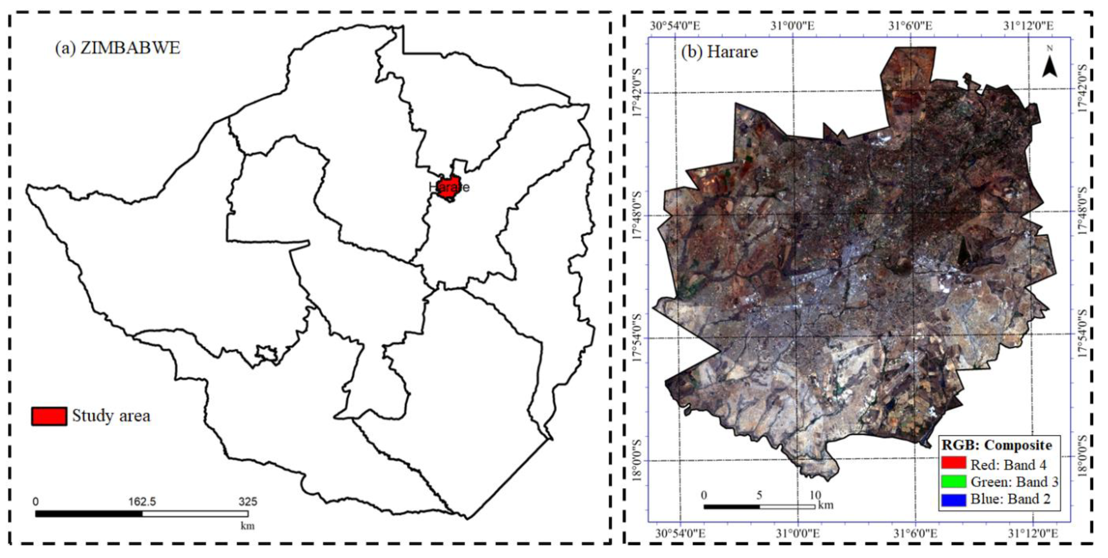
2.1. The City of Harare

Harare (Figure 1) is the largest city in Zimbabwe. The city is fast growing, as indicated by population growth and the expansion of built-up areas for settlement and business activities. The city had a population of 1,435,784 during the 2012 census [55]. The 2022 census revealed that the city’s population had grown to 2,427,209, with the largest number of households (653,562) compared to other cities [56]. According to [57], the expansion of the city has seen a peripheral retreat of natural vegetation, as built-up areas congest around the Central Business District (CBD). However, even within the city’s built-up areas, some open land of varying sizes and fragmentation levels can still be found. Some of them alternate as bare land, croplands, and grasslands in different seasons of the year. The other open lands are occupied by parks and sporting fields, which are well maintained in areas very close to the CBD and in spacious settlements, occupied by middle and high income strata. Settlements in Harare are stratified on the basis of income, with the northern half dominated by spacious low to medium density residential areas, where occupants are perceived to be middle to high income earners [58]. In these areas, land areas are large and green spaces are well maintained throughout the year. On the other, there are varying extents of high density residential areas occupied by low to medium income strata. The land areas in these locations are small, with houses closely packed. This stratum also includes some informal settlements where very small houses are closely packed and built using low quality materials. Informal settlements are also characterized by low roof height, which may affect indoor comfort, especially from a thermal environment perspective. These variations in settlement types and built-up extent affect the distribution of temperatures between and within strata. Hence, understanding these variations is a valuable guide to designing optimal urban climate strategies, as well as ensuring sustainable cities.

2.2. Mapping of Local Climate Zones

A field survey was conducted to identify Local Climate Zones (LCZs) in the city, guided by the standard template as described by Bechtel et al. [15]. The LCZs identified were the compact midrise (LCZ2), the compact lowrise (LCZ3), open midrise (LCZ5), open lowrise (LCZ6), lightweight lowrise (LCZ7), dense forest (LCZA), low plants (LCZD), and water (LCZG). Compact midrise and compact lowrise were mainly found in the CBD and industrial areas congested in the center of the city. Buildings which could be classified as compact highrise and open highrise were also found in and around the CBD. However, they were few and insufficient to constitute a local climate zone and were merged with a closest category. Ground control points of representative samples of each LCZ were collected using a handheld GPS. The points were overlaid on Google Earth imagery coinciding with the date of the Landsat data (used for LCZ mapping). In Google Earth, polygons were digitized to create samples to train classification of each LCZ category as prescribed by the World Urban Database and Access Portal Tool (WUDAPT) procedure [21,59,60]. LCZ mapping was conducted using the Random Forest Classifier in SAGA GIS software, as guided by the WUDAPT procedure. Post-classification accuracy assessment was determined using Overall Accuracy (OA), Kappa (k), Producer Accuracy (PA), and User Accuracy (UA) as quantitative measures.

2.3. Retrieval of Land Surface Temperature Using a Single Channel Algorithm

A single channel algorithm was employed to derive Land Surface Temperature (LST) from Landsat 8′s thermal data (Band 10). Following steps in Bhatti and Tripathis [61], digital numbers of band were converted to radiances (Lλ) using Equation (1):
L λ = M L Q c a l + A L
ML and AL are band-specific multiplicative and additive coefficients obtained from the metadata file downloaded together with imageries, while Qcal is the thermal band digital numbers.
Equation (2) is the Planck’s equation for Landsat 8 used to convert thermal radiances of Band 10 to blackbody of brightness temperature (Tb)
T b = K 2 ln ( K 1 L λ + 1 )
In Equation (2), K1 and K2 are calibration constants taking values of 774.89 and 1321.08 for Band 10 of Landsat 8, respectively [40].
Brightness temperatures do not account for differences in surface properties, as it assumes that all objects have a uniform emissivity of 1. This assumption is not ideal, especially in a city where thermal properties vary within short distances. In order to solve this challenge, brightness temperature is converted to land surface temperature (LST) per pixel, by way of emissivity correction using Equation (3):
L S T = T b [ 1 + ( λ T b σ ) ln ε ]
σ is equivalent to h c λ taking a value of 1.438 × 10⁻² mk, h is Planck’s constant (6.63 × 10⁻³⁴ Js), c is the speed of electromagnetic radiation (3 × 10⁸ ms−1), while σ is the Boltzmann constant (1.38 × 10⁻²³ J/K)—[62]. ε is surface emissivity calculated per every 30 m resolution pixel using Equation (4):
ε = 0.004 P V + 0.986
PV is the proportion of vegetation in a pixel obtained using Equation (5):
P V = [ N D V I N D V I m i n N D V I m a x N D V I m i n ] 2
NDVImax and NDVImin are global maximum and minimum values in the NDVI image, respectively [62]. The normalized difference vegetation index (NDVI) is retrieved from the reflectivity of red ( ρ R e d ) and near-infrared ( ρ N I R ) using Equation (6):
N D V I = ρ N I R ρ R e d ρ N I R + ρ R e d

2.4. Processing of Elevation Data and Retrieval Landsat 8-Derived Indices

A 30 m resolution Digital Elevation Model (DEM) in raster format from an Advanced Space-borne Thermal Emission and Reflection Radiometer (ASTER) corresponding to Harare city was downloaded from the United States Geological Survey’s (USGS) earth explorer website. The clip function in ArcGIS was used to confine the DEM to the boundary of Harare to reduce demand for storage and facilitate analysis. The DEM was used to derive Aspect at 30 m resolution. Landsat data were used to derive MNDWI, NDBaI, NDBI, and UI using Equations (7)–(10) [42,48,50,61,63,64]:
M N D W I = ρ G r e e n ρ S W I R 2 ρ ρ G r e e n + ρ S W I R 2
N D B I = ρ S W I R 2 ρ N I R ρ S W I R 2 ρ N I R
N D B a I = N I R M I R N I R + M I R
U I = S W I R 2 N I R S W I R 2 + N I R
Visual inspection was used to analyze the variations of the physical properties represented by these indices in the city.

2.5. Analysis of LST Variations between and within LCZ

2.5.1. LST Variations between LCZs

Visual inspection of the derived LCZ and LST maps was used to determine the qualitative relationship between LCZs and LST. The Zonal Statistics overlay function in ArcGIS was used to obtain the mean LST of each LCZ category. Furthermore, 1000 points were created for each LCZ and used to extract values from the LST layer. The values obtained were further used to generate boxplots which depicted the variations in LST between and within LCZs. Since LCZs are qualitative classes, quantitative analysis of the relationship between surface temperature and LST was performed using Elevation, Aspect, MNDWI, NDBaI, NDBI, NDVI, and UI. The overlay was employed to obtain the global correlation between LST and each of the factors which influence surface temperature distribution. This was conducted in order to understand the extent to which a factor influences LST, as well as to then establish if the same correlations would stand at individual LCZ scale.
While each LCZ can contribute to either the cooling or warming of the city, understanding how respective sizes affect the overall thermal environment of a city is important. In this study, this was achieved using the Contribution Index (CI), which considers whether a category causes warming or cooling, and its overall significance is determined by its proportion of the entire study area [65]. The Contribution Index for each LCZ category was calculated using Equation (11):
C I = D t × S
Dt is the difference between the average temperature of an LCZ category and the mean LST of the entire study area, S is the proportion of the study area occupied by the LCZ (as a decimal). The CI was also useful to gauge how trends in LCZs of high mitigation value could affect the entire thermal environment of a city.

2.5.2. LST Variations within LCZs

The quantitative relationship between LST and surface properties was also determined using DEM retrievals (Elevation and Aspect) and five land cover indices (MNDWI, NDBaI, NDBI, NDVI, and UI). Using the same 1000 random points per LCZ, additional values were extracted from the seven layers. The correlation between LST and each of the factors was determined for each LCZ category. The strengths of the correlations were used to identify the major causes of LST variations within an LST, while p-values were used to assess the statistical significance of each effect. Analysis was also used to determine if the effects of these factors changed from one LCZ type to another. This was necessary in order to identify the type of development or adjustments needed to avoid excessive LST in each LCZ.

2.6. Summary of Approach Used in This Study

Figure 2 provides a summary of the steps followed in the study, which include LCZ mapping, computation of land surface temperature, retrieval of land surface characteristics, and analyzing their link with spatial structures of land surface temperature. While ground truth data was used for LCZ mapping and accuracy assessment, the study was largely based on freely available remotely sensed data.

3. Results and Discussions

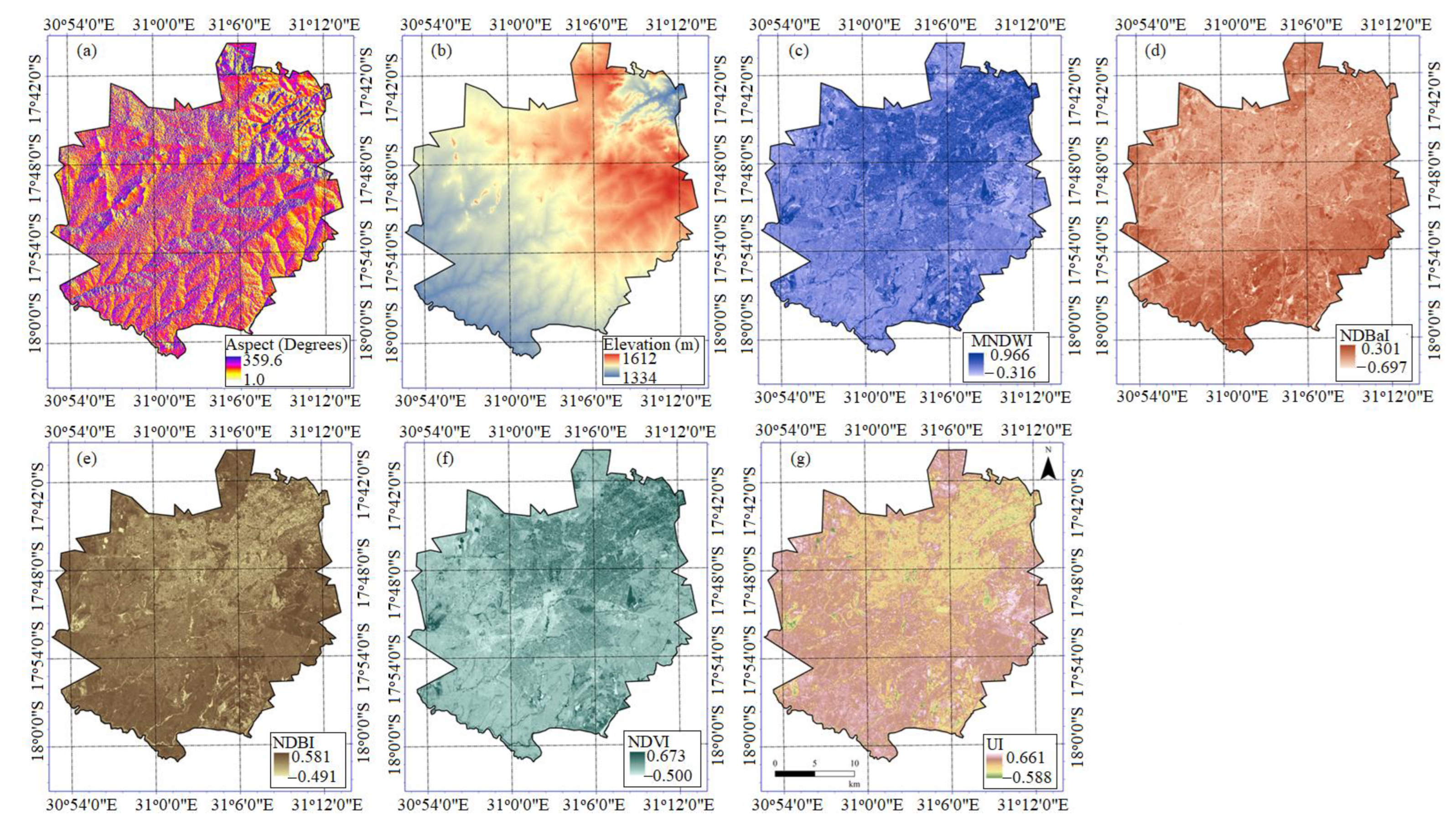
3.1. Distribution of Drivers of Land Surface Temperature Variations in Harare

Visual inspection of Figure 3a shows variations in terms of aspect within short distances. Significant variations in terms of aspect were observed in the northeastern quarter of the city. A southwest to northeast gradient observed in other factors was also evident. Statistical analysis using normalized aspect showed a standard deviation of 0.281 (101.298 m using absolute value without normalization). The city is generally on high ground, with elevation ranging between 1324 and 1612 m, with a standard deviation of 48.145 m (0.173 after normalization) (Figure 3b). There was a general southwest to northeast increase in elevation, with the city almost equally divided into high and low ground stretching from the center of the city. Lowest values of NDVI (Figure 3e) and NDWI (Figure 3f) were concentrated at the center of the city, where NDBaI (Figure 3c), NDBI (Figure 3d) and UI (Figure 3g) were highest. Generally, NDBaI, NDBI, and UI were very high in the southwestern quarter, as well is in the eastern areas of the city, where NDVI and MNDWI values were low. There was an inverse relationship between NDBaI, NDBI, and UI with NDWI and NDVI. The standard deviation was 0.107, 0.086, 0.076, 0.075, and 0.066 for NDVI, UI, NDWI, NDBaI, and NDBI, respectively. This indicated that NDVI followed after Aspect and Elevation as the most variable factors in the city, while variations in UI were also notable.

3.2. Accuracy of LCZ Mapping

LCZs for Harare were mapped with very high accuracy, as indicated by an Overall Accuracy of 92.4% and Kappa index value of 0.92 (Table 1). Producer accuracy ranged between 63.47 and 100%, while User Accuracy ranged between 76.45% (in the Compact midrise LCZ) and 100% (in the Water LCZ). User accuracy was at least 76% for all classes, with a lowest value of 76.45% (in the compact lowrise LCZ) and highest of 100% (in the water LCZ). Dense forest, lightweight lowrise, low plants, open lowrise, and water LCZ were mapped with very high accuracies, as indicated by both Producer and User accuracies greater than 90%.

3.3. Transformed Divergence Separability Index (TDSI)

Separability analysis showed that water was the most separable from other LCZs (Transformed Divergence Separability Index (TDSI) = 2) while compact midrise and compact lowrise had similar spectral characteristics (TDSI = 1.071) (Table 2). Spectral similarity between compact lowrise and compact midrise could be due to the high density of buildings, which was common to both LCZ categories [17]. However, TDSI values were greater than 1.000, mostly between 1.071 and 2.000 for any two paired classes, which indicated that the LCZs were largely easily separable from each other using the ground truth and imagery data.

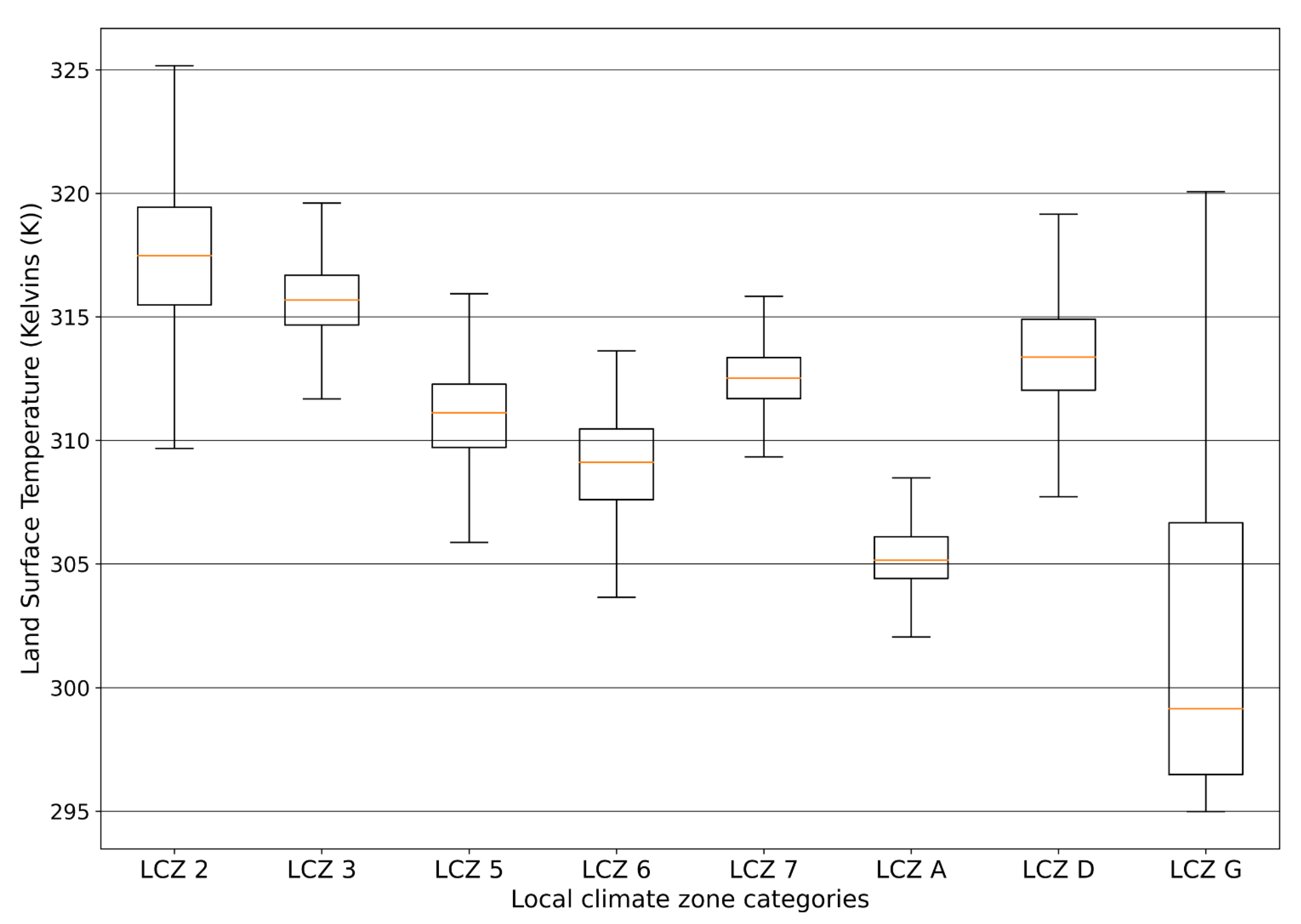
3.4. LCZ Map and Variations of LST in Harare

Figure 4a presents the accuracy LCZ map along with the retrieved LST map for Harare (Figure 4b). The very densely packed built-up LCZ2 and LCZ3 occupied the center of the city, with other categories radiating towards the margins of the city. Another densely built category (LCZ7) occupied much of the southwestern and eastern areas of the city. The sparsely built LCZ5 and LCZ6 occupied a much larger combined area than the densely built-up categories. The northern half and southeastern quarter of the city were dominated by spacious settlement areas. Of the land-cover-based categories, LCZA (dense trees) and LCZG (water) occupied less area and were more fragmented than the low plants category (LCZD). LCZD still dominated the eastern and western flanks of the city and was still visible in other parts of the city. A comparison with Figure 4a,b shows that LSTs were highest in areas corresponding to LCZ2 and LCZ3. Pockets of areas with very high LSTs of the same order as those observed in very densely built LCZs were also observed in other areas, such as in low plants LCZ. Very low LSTs mainly coincided with LCZG, LCZ5, and LCZ6 locations. There was a general southwest to northeast decrease in LST, which was a response to the decrease in the density of buildings in that direction. There was evidence of notably high temperature areas with similar temperature ranges to LCZ2 and LCZ3, mainly in the low plants LCZ.
Figure 5 shows that LCZ 2 was the warmest, followed by LCZ3 and LCZ7. Of the built-up LCZs, LCZ5 and LCZ6 were the coolest, while LCZA and LCZG were the coolest of all categories in the city. LCZD was even warmer than the built-up LCZ5, LCZ6, and LCZ7. LCZ2, LCZD, and LCZG were the most variable, as indicated by long tails, while generally, there were some overlaps.

3.5. Correlation of LST and Indices of Land Surface Characteristics in Harare

At city scale, LST strongly and positively correlated with NDBI (0.659) and UI (0.769), while there was some positive correlation with NDBaI (0.050) (Figure 6). On the other hand, there was a strong negative correlation with NDVI (−0.786) and MNDWI (−0.741), while it was weak with Aspect (−0.019) and Elevation (−0.130).

3.6. Relative Contribution of LCZs to Warming and Cooling in Harare

Although LCZG has key heat mitigation values, the limited area for such category reduces its contribution towards the cooling of the city (Table 3). Although the category has become fragmented, LCZA (dense trees) has remained an important agent for surface cooling in the city. A pronounced cooling contribution (CI = −0.654) in the city comes from LCZ6, which is sparsely built with high vegetation fraction. LCZ2 is the warmest, but its contribution to the net heating of the city (CI = 0.023) is limited by the small proportion of the city it occupies (0.35%).

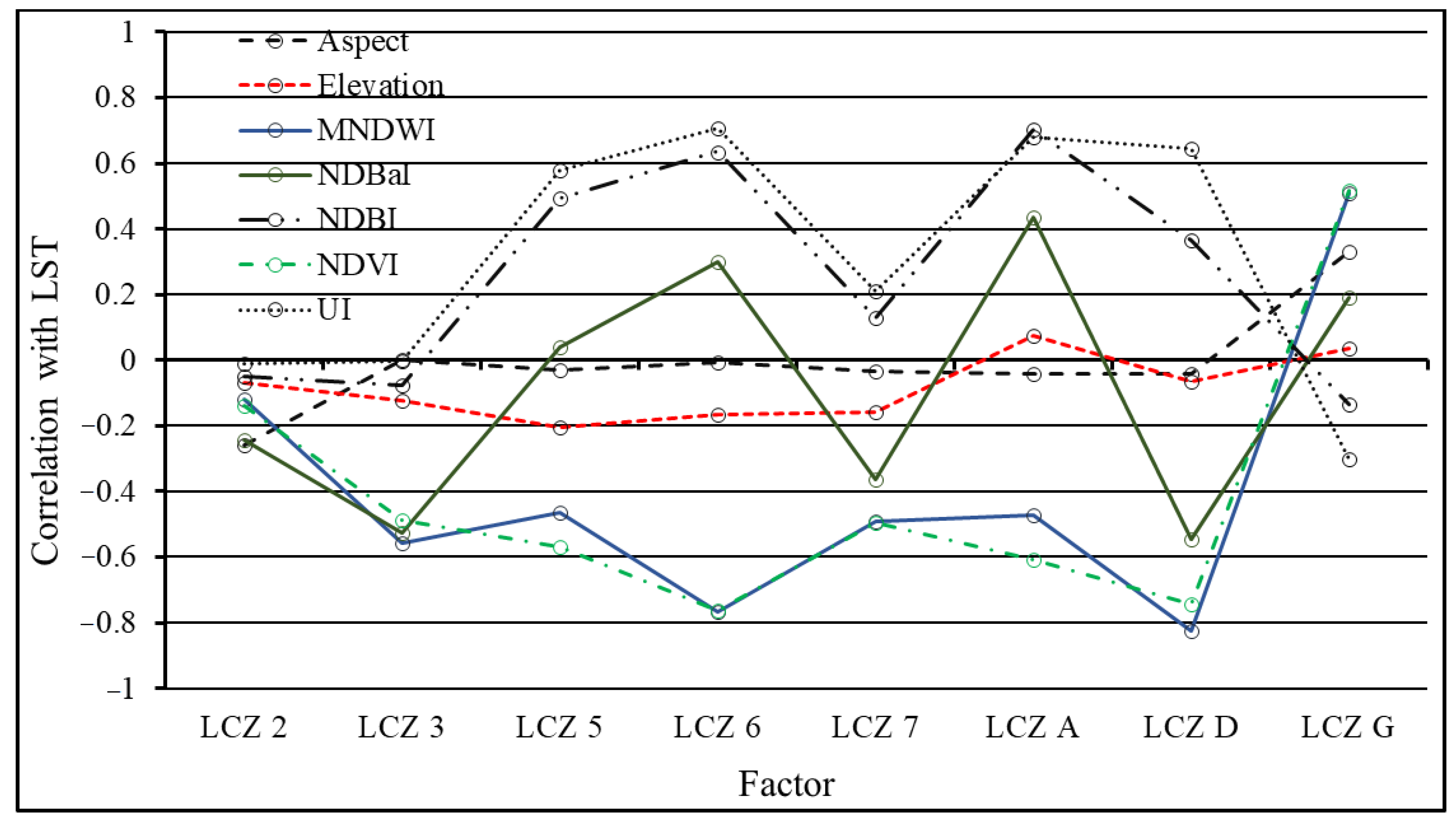
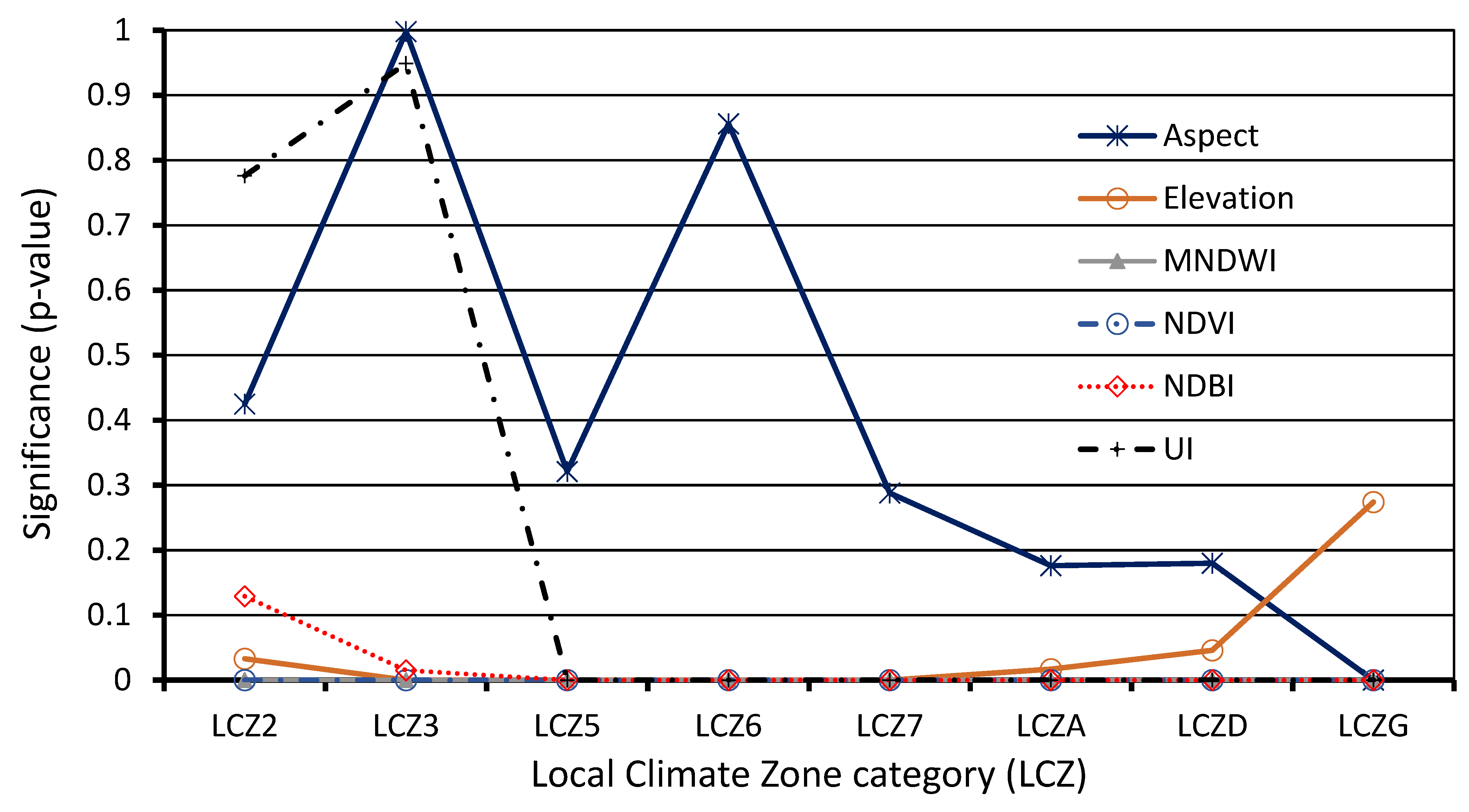
3.7. Intra-LCZ Correlation of LST and Indices of Land Surface Characteristics

Strength and direction of correlations of LST with Aspect, Elevation, MNDWI, NDBaI, NDBI, NDVI, and UI varied between LCZs (Figure 7). This indicated that each LCZ was affected by factors in its own unique way. In LCZ2 and LCZ3, LST negatively and weakly correlated with Aspect, Elevation, MNDWI, NDBaI, NDBI, NDVI, and UI, as evidenced by low correlation coefficients (below 0.3). In LCZ5, there was some negative correlation between LST and Elevation, and negative correlation between LST and MNDWI (r close to −0.5) and NDVI (r close to −0.6). A similar correlation between LST and these factors was also recorded in LCZ7.
Stronger negative correlation between LST and Elevation, and MNDWI and NDVI, was recorded in LCZ6. The correlation between Elevation and LST was very low in LCZA. In LCZD, the extent of urbanization had the highest positive correlation with LST, while surface wetness and vegetation abundance had the strongest negative correlation with LST. Similar to LCZ3 and LCZ7, LST decreased with bareness in LCZD. The thermal behavior of LCZG (water) was adversely affected by the increase in NDVI, NDBI, and NDBaI, resulting in warming.
Figure 8 shows the influence (significant if p-value < 0.05) of Aspect, Elevation, surface wetness (MNDWI), bareness (NDBaI), built-up extent (NDBI), vegetation abundance and health (NDVI), and urbanization extent (UI) on LST within a LCZ. Aspect, built-up extent (NDBI), and urbanization extent weakly influenced LST in LCZ2. Similarly, the extent of urbanization was also not a significant factor governing variations of LST in LCZ3, which is also heavily built-up. In LCZ5, other factors significantly influenced LST, with the exception Aspect and bareness (NDBaI). In LCZ6, LCZ7, LCZA, and LCZD, all other factors significantly affected the LSTs spatial distribution (p < 0.05), with the exception of Aspect (p = 0.18). On water bodies (LCZG), all other factors significantly affected LST distribution, except elevation (p = 0.274). The significance of Aspect in affecting the spatial structure of LST was only high in LCZG.

3.8. Comparison of LST Drivers at City and Intra-LCZ Scales

At the city scale, Aspect and Elevation had very small and negative correlations with LST (correlation coefficients of about −0.15). This pattern was replicated even at the intra-LCZ scale. The magnitude of LST correlations with NDBI, NDVI, NDBaI, MNDWI, and UI exceeded 0.6 at the city scale. The importance of these factors in explaining LST variations with LCZs was variable. As such, the correlation of LST with UI was high (correlation coefficient > 0.6) only in LCZ5, LCZ6, LCZA, and LCZD.

Discussion of Findings

The LCZs were mapped with high accuracy using Landsat 8 multispectral data using the WUDAPT approach. The high accuracy of LCZ mapping can be attributed to Landsat 8′s high quality data [66,67,68,69], as well as Random Forest classifier’s superior performance in mapping land surface characteristics [70,71,72]. The LULC types and spatial structures were largely distinct, resulting in adequate differentiation between the different LCZ categories. The built-up LCZs were also adequately distinguishable. This is consistent with Wania et al. (2014) [58], who noted that Harare had built-up categories which differed in terms of the density of buildings, the sizes of land units, and the distribution of vegetation within the built-up categories. The LCZ map emphasized the differences in built-up densities between the northern and southern areas with spaced out homes and abundant vegetation in the northern half [57,58]. In agreement with Kamusoko et al. (2013) [57], historical growth-induced LULC changes have pushed unbuilt areas towards the margins of the city. The compact midrise and compact lowrise occupy less area than the other built-up LCZs. This can be attributed to high cost and intensive use of land, as these areas correspond to the CBD with more vertical developments and closely packed business units.
There was an inverse relationship between NDBaI, NDBI, and UI with NDWI and NDVI. The increase in LST with the decrease in NDVI concurs with Hansen et al. [73], that changes in vegetation distribution affect climate regulation services offered by vegetation cover areas, such as forests. As an area experiences an increase in urban fabrics, the temperature moderation value of vegetation diminishes, which explains surface warming with the increase in NDBI and UI. The inverse relationship between LST and NDWI explains the implication of vegetation health on their heat mitigation value. Where vegetation is healthy, the plant cells will be turgid and able to transpire, resulting in heat reduction by latent heat transfer [74,75,76]. Additionally, surface wetness and abundance of water of any land surface has a marked temperature reduction effect [40,77]. Our findings indicated that surface wetness and abundance of healthy vegetation were the most pronounced surface heat mitigation measures. On the other hand, the increase in built-up area and urban fabric were the most significant causes of surface warming. However, the increase in bareness also had some warming effects, while the increase in Aspect and Elevation had some cooling effect on LSTs. Generally, built-up density, surface water and vegetation quality, and abundance were the major controlling factors of LST at the city scale in Harare. Buildings and other urban fabrics absorb a lot of heat during the day, and their effect increases with the density of the buildings and the proportion of urban fabrics, such as pavements and tarmacs in a unit area [78,79,80,81].
A comparison of thermal characteristics between LCZs showed that LSTs were highest in areas corresponding to LCZ2 and LCZ3. Pockets of areas with very high LSTs of the same order as those observed in very densely built LCZs were also observed in other areas, such as in low plants LCZ. These were attributed to localized features with high heat absorption capacity, such as dry and impervious surfaces, which elevated surface temperatures in areas of occurrence. Very low LSTs mainly coincided with LCZG, LCZ5, and LCZ6 locations, where either density of urban fabrics was low, or vegetation fraction was high, or surface water content was high. There was a general southwest to northeast decrease in LST, which was a response to the decrease in the density of buildings in that direction. There was evidence of notably high temperature areas with similar temperature ranges to LCZ2 and LCZ3, mainly in the low plants LCZ. The study was conducted during the hot season, when vegetation in some areas is dry and semi-bare to bare low plants areas, hence the elevated temperatures. The LCZ mapping scheme used in this study produced a static map which did not adapt to seasonal changes in vegetation characteristics, which affect land surface and air temperature variations. As such, during the same hot season, variations in vegetation characteristics (greenness, abundance, and health) vary within the city. For example, in built-up LCZs occupied by medium and high income strata, as well as in well maintained greenspaces such as urban parks and sporting fields, the quality of the vegetation may differ from that in natural areas.
LCZ 2 was the warmest, followed by LCZ3 and LCZ7, while, of the built-up LCZs, LCZ5 and LCZ6 were the coolest. LCZA and LCZG were the coolest of all categories in the city. LCZD was even warmer than the built-up LCZ5, LCZ6, and LCZ7. LCZ2, LCZD, and LCZG were the most variable, as indicated by their long tails, while, generally, there were some overlaps. Previous studies have also identified LCZ2 (compact midrise) as the warmest due to the high density of buildings and high sky view factor, even when compared to compact highrise areas [28,82]. The high LST in some LCZD areas was because some of the areas had dry grass and were semi-barren to barren. In such areas, the cooling effect of vegetation was eliminated due to the seasonality of vegetation. This finding is consistent with Badaro-saliba et al. [31], who also determined that the importance of factors to LST variations changed with seasons, such as in Beirut city in Lebanon. The cooling effect of vegetation was evident in the built-up LCZ5, LCZ6, and LCZ7, where buildings were widely spaced and separated by healthy and well-maintained vegetation. This was in agreement with Zhou et al. [23], who noted that LCZs with high vegetation density had low LSTs. The presence of vegetation in LCZ5 and LCZ6 compensates for warming due to large buildings and impervious surfaces in these areas [31]. Similar to Dimitrov et al. (2021) [18], in Sofia, Bulgaria, LCZG (Water) was the coolest, while built-up categories were warmest. The wide variations in LST in LCZG (water) could indicate spatial variations in water quality, as well as the mixed pixel effect on LST, given the small area covered by the LCZ in the city. At a 100 m resolution of Landsat 8′s thermal data, it was possible for an LST pixel in water areas to include other LCZs and widen the variations.
Although LCZG has key heat mitigation values, the limited area for such a category reduces its contribution towards the cooling of the city. LCZ2 was the warmest, but its contribution to the net heating of the city was low due to the small proportion of the city it occupies. Similarly, in Sophia, Bulgaria, LCZ9 had the highest temperature, but its contribution to the city’s temperature was limited by the insignificant area it occupied [18]. The largest contributors to the heat load of the city were LCZ3 and LCZ7 with CI determination values, while LCZ7 is cooler than LCZ3, but has a larger CI due to the large proportion of the city it occupies compared to that occupied by LCZ3.
The strength and direction of correlations of LST with Aspect, Elevation, MNDWI, NDBaI, NDBI, NDVI, and UI varied between LCZs. This indicated that each LCZ was affected by the same factors in its own unique ways. In LCZ2 and LCZ3, LST negatively and weakly correlated with Aspect, Elevation, MNDWI, NDBaI, NDBI, NDVI, and UI, as evidenced by low correlation coefficients. This indicated that cool spots within LCZ2 and LCZ3 were bare, wet, vegetated, and sparsely built-up areas. The study was conducted during the dry season and the contribution of surface wetness to LST with these densely built-up LCZs was negligible; hence, the low correlation with MNDWI. Similarly, the vegetation areas occupy close to negligible proportions in the LCZ, such that their cooling effect is very small. However, even though the effect is small, it still emphasizes the value of urban greenery and surface wetness in reducing LSTs, even within densely built-up areas.
The observed strong correlation between NDVI and LST in sparsely built and natural land covers is attributed to the cooling effect of canopy transpiration [42]. The observation determined the same heat mitigation value of increasing surface wetness and vegetation within built-up areas also indicated in recent studies [23,31,82,83]. In LCZ5 and LCZ6, increasing bareness and built-up proportion were the most prominent factors (highly so in LCZ6) in causing surface warming. The contribution of urban fabric had some influence in increasing surface warming, with a larger effect in LCZ6 than in LCZ5. Conversely, although bareness and built-up extent caused warming in LCZ7, their effect was weaker (low correlation with LST) than the cooling effect of surface water and vegetation cover. Nassar et al. [34] also observed that surface wetness due to proximity to water bodies has significant influence on LST. In terms of LCZA built-up extent, bareness and increasing urban fabric had marked contributions to surface warming. Increasing surface wetness and vegetation cover were the most significant surface cooling approaches in LCZA. There was very low correlation between elevation and LST in LCZA, while the extent of urbanization had the highest positive correlation with LST in LCZD. On the other hand, in LCZD, surface wetness and vegetation abundance had the strongest negative correlation with LST. Similar to LCZ3 and LCZ7, LST decreased with bareness in LCZD. The increase in NDVI, NDBI, and NDBaI, resulting in warming, adversely affected the thermal behavior of LCZG (water). This implies that factors such as water plants compromise the cooling effect that would be attained when an area is covered by a water body. This finding is supported by Sun et al. [48], who noted that pure and polluted water reduces and increases LST, respectively. This implies that the maintenance of high water quality in an area is an important heat mitigation measure. In LCZ2, Aspect, built-up extent (NDBI), and urbanization extent did not have a significant influence of LST. This could be attributed to the built-up and urbanization extent being high and almost homogeneous. Competition between built-up and other functions is minimal, as the region is extensively and compactly constructed, with an almost uniform distribution of LST. This also explains why the correlation of LST with NDBI and UI is weak and insignificant (p > 0.05) in the densely built-up LCZ2 and LCZ3.
The magnitude of LST correlations with NDBI, NDVI, NDBaI, MNDWI, and UI exceeded 0.6 at the city scale. This indicated that the built-up/urbanization extent, vegetation distribution, and surface water explain the variations in LST at the city scale. As such, LCZs with a high density of buildings had higher LSTs than those with spaced out buildings surrounded by vegetation. The importance of these factors in explaining LST variations with LCZs was variable. As such, the correlation of LST with UI was only high in LCZ5, LCZ6, LCZA, and LCZD. In LCZs that are almost uniformly densely built-up, UI was almost homogeneous and no longer a factor controlling LST variations. At the intra-LCZ scale, variations of LST were mostly explained by NDVI, MNDWI, NDBaI, NDBI, and UI. At this scale, NDVI, MNDWI, UI, and NDBI had more control of LST variations than the other factors, and mostly so in LCZs which were not densely built. On the other hand, within densely built-up LCZs, LSTs were low in places with vegetation, surface water, and in barren lands. these places absorb less heat than the built-up sections and, in the cases of vegetation and surface water, they aid cooling by latent heat transfer.

4. Shortcomings of the Study

The study was not exhaustive of all possible factors that can influence land surface temperature within and between LCZs. For instance, variations in wind direction and wind speed have potential to influence surface temperature dynamics, and they were not directly considered in this study. Additionally, other factors such as the effect of shading have influence on LST, which were not considered. Due to the absence of in situ measurements in the study area, LSTs were not assessed in terms of accuracy.

5. Conclusions and Recommendations

This study mapped LCZ and used remotely sensed land surface properties to determine the major drivers of LST variations between and within LCZ in Harare. The study established that the RF algorithm is effective for LCZ classification, as it mapped a complex city with high accuracy. LST varied between LCZs with increased warming as a consequence of the decrease in vegetation proportion, decrease in surface wetness, and increase in built-up extent. The densely built-up LCZ2 and LCZ3 were the warmest, while dense forest and water LCZs were the coolest due to cooling by latent heat transfer. Therefore, urbanization extent, surface wetness and distribution, and health of vegetation were the major determinants of variations in LST between LCZs. Intra-LCZ analysis showed that factors such as increased bareness and elevation made low but significant contributions to LST spatial structure. The effect of these contributing factors was not uniform in strength and direction (warming or cooling) in affecting LST across all LCZs. In the densely built-up LCZ2 and LCZ3, the increase in wetness, bareness, and vegetation density led to a reduction in LST, while changes in terms of built-up extent had no effect, given that the area is almost homogenous and densely built. In other built up LCZs, the increase in built-up extent and urbanization extent were the major causes of warming, while vegetation and surface wetness caused significant cooling. The expansion of buildings into dense vegetation areas caused the most warming than any other transitions in the city. Based on the Contribution Index, we concluded that the heat mitigation value of vegetation and water areas in a city is reduced by their relatively small and diminishing coverage compared to surfaces with warming effects. Additionally, a conclusion was drawn that a reduction in the health of vegetation in areas, as well as the quality of water, reduces their heat mitigation value. The influence of surface characteristics on LST varied at the inter-LCZ scale compared to patterns observed at the intra-LCZ scale. Based on these findings, this study recommends that surface heat mitigation approaches must differ from one LCZ to another, with a consideration of how LSTs respond to surface characteristics. Future studies should consider high resolution datasets (>10 m) to understand the effect of elevation and aspect, as 30 m resolution may be insufficient for this highly dynamic aspect.

Author Contributions

Conceptualization, T.D.M., O.M. and J.O.; methodology, T.D.M.; software, T.D.M.; validation, T.D.M., O.M. and J.O.; formal analysis, T.D.M.; investigation, T.D.M., O.M. and J.O.; resources, T.D.M., O.M. and J.O.; data curation, T.D.M., O.M. and J.O.; writing—original draft preparation, T.D.M.; writing—review and editing, T.D.M., O.M. and J.O.; visualization, T.D.M.; supervision, O.M. and J.O.; project administration, O.M. and J.O.; funding acquisition, T.D.M., O.M. and J.O. All authors have read and agreed to the published version of the manuscript.

Funding

We acknowledge the National Research Foundation (NRF) of South Africa and the Germany DAAD climapAfrica for funding the research. This work was funded by the National Research Foundation of South Africa (NRF) Research Chair in Land Use Planning and Management (Grant Number: 84157). The research of this article was supported by DAAD within the framework of the climapAfrica programme with funds of the Federal Ministry of Education and Research. The publisher is fully responsible for the content.

Informed Consent Statement

Not applicable.

Data Availability Statement

Remotely sensed data used in this study can be freely downloaded from United States Geological Survey (USGS) Earth Explorer website (www.earthexplorer.usgs.gov (accessed on 14 Septemper 2022)). The training data used to map LCZ have been uploaded on the WUDAPT website (https://lcz-generator.rub.de/factsheets/3eb90c0ab4210886bdd0b23f1fc7dccae893c005/3eb90c0ab4210886bdd0b23f1fc7dccae893c005_factsheet.html (accessed on 18 September 2022)).

Acknowledgments

We acknowledge the Climate Modeling Group of the climapAfrica fellowship for inputs during virtual presentations which contributed to the quality of this manuscript. We thank the Discipline of Geography, School of Agricultural, Earth and Environmental Sciences in Pietermaritzburg, South Africa for availing a fruitful research environment. The Department of Space Science and Applied Physics at University of Zimbabwe also provided a working environment for this research.

Conflicts of Interest

The authors declare no conflict of interest.

References

  1. Zhang, H.; Qi, Z.F.; Ye, X.Y.; Cai, Y.B.; Ma, W.C.; Chen, M.N. Analysis of land use/land cover change, population shift, and their effects on spatiotemporal patterns of urban heat islands in metropolitan Shanghai, China. Appl. Geogr. 2013, 44, 121–133. [Google Scholar] [CrossRef]
  2. Zhou, X.; Wang, Y.C. Spatial-temporal dynamics of urban green space in response to rapid urbanization and greening policies. Landsc. Urban Plan. 2011, 100, 268–277. [Google Scholar] [CrossRef]
  3. Acharya, T.D.; Parajuli, J.; Shahi, K.; Poudel, D.; Yang, I. Extraction and Modelling of Spatio-Temporal Urban Change in Kathmandu Valley. Int. J. IT Eng. Appl. Sci. Res. 2015, 4, 1–11. [Google Scholar]
  4. Jalan, S.; Sharma, K. Spatio-temporal assessment of land use/ land cover dynamics and urban heat island of Jaipur city using satellite data. Int. Arch. Photogramm. Remote Sens. Spat. Inf. Sci. ISPRS Arch. 2014, XL-8, 767–772. [Google Scholar] [CrossRef] [Green Version]
  5. Valdiviezo-N, J.C.; Téllez-Quiñones, A.; Salazar-Garibay, A.; López-Caloca, A.A. Built-up index methods and their applications for urban extraction from Sentinel 2A satellite data: Discussion. J. Opt. Soc. Am. A 2018, 35, 35. [Google Scholar] [CrossRef] [PubMed]
  6. Polydoros, A.; Cartalis, C. Assessing thermal risk in urban areas—An application for the urban agglomeration of Athens. Adv. Build. Energy Res. 2014, 8, 74–83. [Google Scholar] [CrossRef]
  7. McMichael, A.J.; Woodruff, R.E.; Hales, S. Climate change and human health: Present and future risks. Lancet 2006, 367, 859–869. [Google Scholar] [CrossRef]
  8. Harlan, S.L.; Ruddell, D.M. Climate change and health in cities: Impacts of heat and air pollution and potential co-benefits from mitigation and adaptation. Curr. Opin. Environ. Sustain. 2011, 3, 126–134. [Google Scholar] [CrossRef]
  9. Pérez-Andreu, V.; Aparicio-Fernández, C.; Martínez-Ibernón, A.; Vivancos, J.L. Impact of climate change on heating and cooling energy demand in a residential building in a Mediterranean climate. Energy 2018, 165, 63–74. [Google Scholar] [CrossRef]
  10. Guhathakurta, S.; Gober, P. The impact of the Phoenix urban heat Island on residential water use. J. Am. Plan. Assoc. 2007, 73, 317–329. [Google Scholar] [CrossRef]
  11. Fu, Y.; Lu, X.; Zhao, Y.; Zeng, X.; Xia, L. Assessment impacts of weather and land use/land cover (LULC) change on urban vegetation net primary productivity (NPP): A case study in guangzhou, China. Remote Sens. 2013, 5, 4125–4144. [Google Scholar] [CrossRef]
  12. Mbithi, D.M.; Demessie, E.T.; Kashiri, T. The Impact of Land Use Land Cover (LULC) Changes on Land Surface Temperature (LST); A Case Study of Addis Ababa City, Ethiopia; Kenya Meteorological Services: Nairobi, Kenya, 2006. [Google Scholar]
  13. Ullah, S.; Ahmad, K.; Sajjad, R.U.; Abbasi, A.M.; Nazeer, A.; Tahir, A.A. Analysis and simulation of land cover changes and their impacts on land surface temperature in a lower Himalayan region. J. Environ. Manag. 2019, 245, 348–357. [Google Scholar] [CrossRef] [PubMed]
  14. Shugar, D.H.; Jacquemart, M.; Shean, D.; Bhushan, S.; Upadhyay, K.; Sattar, A.; Schwanghart, W.; McBride, S.; De Vries, M.V.W.; Mergili, M. A massive rock and ice avalanche caused the 2021 disaster at Chamoli, Indian Himalaya. Science 2021, 373, 300–306. [Google Scholar] [CrossRef]
  15. Bechtel, B.; Langkamp, T.; Böhner, J.; Daneke, C.; Oßenbrügge, J.; Schempp, S. Classification and Modelling of Urban Micro-Climates Using Multisensoral and Multitemporal Remote Sensing Data. ISPRS—Int. Arch. Photogramm. Remote Sens. Spat. Inf. Sci. 2012, XXXIX-B8, 463–468. [Google Scholar] [CrossRef] [Green Version]
  16. Demuzere, M.; Bechtel, B.; Mills, G. Urban Climate Global transferability of local climate zone models. Urban Clim. 2019, 27, 46–63. [Google Scholar] [CrossRef]
  17. Bechtel, B.; Demuzere, M.; Mills, G.; Zhan, W.; Sismanidis, P.; Small, C.; Voogt, J. Urban Climate SUHI analysis using Local Climate Zones—A comparison of 50 cities. Urban Clim. 2019, 28, 100451. [Google Scholar] [CrossRef]
  18. Dimitrov, S.; Popov, A.; Iliev, M. An Application of the LCZ Approach in Surface Urban Heat Island Mapping in Sofia, Bulgaria. Atmosphere 2021, 12, 1370. [Google Scholar] [CrossRef]
  19. Cai, M.; Ren, C.; Xu, Y.; Dai, W.; Wang, X.M. Local Climate Zone Study for Sustainable Megacities Development by Using Improved WUDAPT Methodology—A Case Study in Guangzhou. Procedia Environ. Sci. 2016, 36, 82–89. [Google Scholar] [CrossRef] [Green Version]
  20. Cai, M.; Ren, C.; Xu, Y.; Lau, K.K.; Wang, R. Urban Climate Investigating the relationship between local climate zone and land surface temperature using an improved WUDAPT methodology—A case study of Yangtze River Delta, China. Urban Clim. 2017, 24, 485–502. [Google Scholar] [CrossRef]
  21. Danylo, O.; See, L.; Bechtel, B.; Schepaschenko, D.; Fritz, S. Contributing to WUDAPT: A Local Climate Zone Classification of Two Cities in Ukraine. IEEE J. Sel. Top. Appl. Earth Obs. Remote Sens. 2016, 9, 1841–1853. [Google Scholar] [CrossRef] [Green Version]
  22. Cai, M.; Ren, C.; Xu, Y. Investigating the relationship between Local Climate Zone and land surface temperature. In Proceedings of the 2017 Joint Urban Remote Sensing Event (JURSE), Dubai, United Arab Emirates, 6–8 March 2017; pp. 1–4. [Google Scholar] [CrossRef]
  23. Zhou, X.; Okaze, T.; Ren, C.; Cai, M.; Ishida, Y.; Watanabe, H.; Mochida, A. Evaluation of urban heat islands using local climate zones under the influences of sea-land breeze. Sustain. Cities Soc. 2020, 55, 102060. [Google Scholar] [CrossRef]
  24. Al Kafy, A.; Dey, N.N.; Al Rakib, A.; Rahaman, Z.A.; Nasher, N.M.R.; Bhatt, A. Modeling the relationship between land use/land cover and land surface temperature in Dhaka, Bangladesh using CA-ANN algorithm. Environ. Chall. 2021, 4, 100190. [Google Scholar] [CrossRef]
  25. Tursilowati, L. Urban Climate Analysis on The Land Use and Land Cover Change (LULC) in Bandung-Indonesia with Remote Sensing and GIS. In Proceedings of the United Nation/Austria/ESA Symposium on Space Tools and Solutions for Monitoring the Atmosphere in Support of Sustainable Development, Graz, Austria, 11–14 September 2007; pp. 11–14. [Google Scholar]
  26. Tyubee, B.T.; Anyadike, R.N.C. Investigating the Effect of Land Use / Land Cover on Urban Surface Temperature in Makurdi, Nigeria. In Proceedings of the ICUC9—9th International Conference on Urban Climate Jointly with 12th Symposium on the Urban Environment, Toulouse, France, 20–24 July 2015. [Google Scholar]
  27. Tran, D.X.; Pla, F.; Latorre-Carmona, P.; Myint, S.W.; Caetano, M.; Kieu, H.V. Characterizing the relationship between land use land cover change and land surface temperature. ISPRS J. Photogramm. Remote Sens. 2017, 124, 119–132. [Google Scholar] [CrossRef] [Green Version]
  28. Fricke, C.; Pongrácz, R.; Gál, T.; Savić, S.; Unger, J. Using local climate zones to compare remotely sensed surface temperatures in temperate cities and hot desert cities. Morav. Geogr. Rep. 2020, 28, 48–60. [Google Scholar] [CrossRef]
  29. Mushore, T.D.; Dube, T.; Manjowe, M.; Gumindoga, W.; Chemura, A.; Rousta, I.; Odindi, J.; Mutanga, O. Remotely sensed retrieval of Local Climate Zones and their linkages to land surface temperature in Harare metropolitan city, Zimbabwe. Urban Clim. 2019, 27, 259–271. [Google Scholar] [CrossRef]
  30. Stewart, I.D.; Oke, T.R.; Krayenhoff, E.S. Evaluation of the “local climate zone” scheme using temperature observations and model simulations. Int. J. Climatol. 2014, 34, 1062–1080. [Google Scholar] [CrossRef]
  31. Badaro-saliba, N.; Adjizian-gerard, J.; Zaarour, R.; Najjar, G. LCZ scheme for assessing Urban Heat Island intensity in a complex urban area (Beirut, Lebanon). Urban Clim. 2021, 37, 100846. [Google Scholar] [CrossRef]
  32. Zhao, C.; Jensen, J.L.R.; Weng, Q.; Currit, N. Use of Local Climate Zones to investigate surface urban heat islands in Texas Use of Local Climate Zones to investigate surface urban heat islands in Texas ABSTRACT. GIScience Remote Sens. 2020, 57, 1083–1101. [Google Scholar] [CrossRef]
  33. Zhang, X.; Estoque, R.C. Capturing urban heat island formation in a subtropical city of China based on Landsat images: Implications for sustainable urban development. Environ. Monit. Assess. 2021, 193, 130. [Google Scholar] [CrossRef]
  34. Nassar, A.K.; Blackburn, G.A.; Whyatt, J.D. International Journal of Applied Earth Observation and Geoinformation Dynamics and controls of urban heat sink and island phenomena in a desert city: Development of a local climate zone scheme using remotely-sensed inputs. Int. J. Appl. Earth Obs. Geoinf. 2016, 51, 76–90. [Google Scholar] [CrossRef]
  35. Budhiraja, B.; Gawuc, L.; Agrawal, G. Seasonality of Surface Urban Heat Island in Delhi City Region Measured by Local Climate Zones and Conventional Indicators. IEEE J. Sel. Top. Appl. Earth Obs. Remote Sens. 2019, 12, 5223–5232. [Google Scholar] [CrossRef]
  36. Dian, C.; Pongrácz, R.; Dezső, Z.; Bartholy, J. Annual and monthly analysis of surface urban heat island intensity with respect to the local climate zones in Budapest. Urban Clim. 2020, 31, 100573. [Google Scholar] [CrossRef]
  37. Farina, A. Exploring the Relationship between Land Surface Temperature and Vegetation Abundance for Urban Heat Island Mitigation in Seville, Spain. LUMA-. GIS Thesis, Lund University, Lund, Sweden, 2012; p. 50. [Google Scholar]
  38. Buyadi, S.N.A.; Mohd, W.M.N.W.; Misni, A. Impact of vegetation growth on urban surface temperature distribution. IOP Conf. Ser. Earth Environ. Sci. 2014, 18, 1627–1634. [Google Scholar] [CrossRef] [Green Version]
  39. Zhang, X.; Zhong, T.; Feng, X.; Wang, K. Estimation of the relationship between vegetation patches and urban land surface temperature with remote sensing. Int. J. Remote Sens. 2009, 30, 2105–2118. [Google Scholar] [CrossRef]
  40. Rasul, A.; Balzter, H.; Smith, C. Spatial variation of the daytime Surface Urban Cool Island during the dry season in Erbil, Iraqi Kurdistan, from Landsat 8. Urban Clim. 2015, 14, 176–186. [Google Scholar] [CrossRef] [Green Version]
  41. McFeeters, S.K. The use of the Normalized Difference Water Index (NDWI) in the delineation of open water features. Int. J. Remote Sens. 1996, 17, 1425–1432. [Google Scholar] [CrossRef]
  42. Karnieli, A.; Agam, N.; Pinker, R.T.; Anderson, M.; Imhoff, M.L.; Gutman, G.G.; Panov, N.; Goldberg, A. Use of NDVI and land surface temperature for drought assessment: Merits and limitations. J. Clim. 2010, 23, 618–633. [Google Scholar] [CrossRef]
  43. Gandhi, G.M.; Parthiban, S.; Thummalu, N.; Christy, A. Ndvi: Vegetation change detection using remote sensing and gis—A case study of Vellore District. Procedia Procedia Comput. Sci. 2015, 57, 1199–1210. [Google Scholar] [CrossRef] [Green Version]
  44. Kostadinov, T.S.; Schumer, R.; Hausner, M.; Bormann, K.J.; Gaffney, R.; McGwire, K.; Painter, T.H.; Tyler, S.; Harpold, A.A. Watershed-scale mapping of fractional snow cover under conifer forest canopy using lidar. Remote Sens. Environ. 2019, 222, 34–49. [Google Scholar] [CrossRef]
  45. Muhuri, A.; Gascoin, S.; Menzel, L.; Kostadinov, T.S.; Harpold, A.A.; Sanmiguel-Vallelado, A.; López-Moreno, J.I. Performance Assessment of Optical Satellite-Based Operational Snow Cover Monitoring Algorithms in Forested Landscapes. IEEE J. Sel. Top. Appl. Earth Obs. Remote Sens. 2021, 14, 7159–7178. [Google Scholar] [CrossRef]
  46. Zha, Y.; Gao, J.; Ni, S. Use of normalized difference built-up index in automatically mapping urban areas from TM imagery. Int. J. Remote Sens. 2003, 24, 583–594. [Google Scholar] [CrossRef]
  47. Xu, H. Modification of normalised difference water index (NDWI) to enhance open water features in remotely sensed imagery. Int. J. Remote Sens. 2006, 27, 3025–3033. [Google Scholar] [CrossRef]
  48. Sun, Q.; Wu, Z.; Tan, J. The relationship between land surface temperature and land use/land cover in Guangzhou, China. Environ. Earth Sci. 2012, 65, 1687–1694. [Google Scholar] [CrossRef]
  49. Huang, Q.; Xu, H.; Yang, X.; Shi, P. Study of impacts of urbanization process on phenology using multisource satellite data. In Proceedings of the American Society for Photogrammetry and Remote Sensing Annual Conference 2009 (ASPRS 2009), Baltimore, Maryland, 9–13 March 2009; Volume 1, pp. 300–305. [Google Scholar]
  50. Mushore, T.D.; Odindi, J.; Dube, T.; Mutanga, O. Prediction of future urban surface temperatures using medium resolution satellite data in Harare metropolitan city, Zimbabwe. Build. Environ. 2017, 122, 397–410. [Google Scholar] [CrossRef]
  51. Kayet, N.; Pathak, K.; Chakrabarty, A.; Sahoo, S. Urban heat island explored by co-relationship between land surface temperature vs multiple vegetation indices. Spat. Inf. Res. 2016, 24, 515–529. [Google Scholar] [CrossRef]
  52. Lee, L.; Chen, L.; Wang, X.; Zhao, J. Use of Landsat TM/ETM+ data to analyze urban heat island and its relationship with land use/cover change. In Proceedings of the 2011 International Conference on Remote Sensing, Environment and Transportation Engineering, Nanjing, China, 24–26 June 2011; pp. 922–927. [Google Scholar] [CrossRef]
  53. Li, H.; Liu, Q. Comparison of NDBI and NDVI as indicators of surface urban heat island effect in MODIS imagery. Int. Conf. Earth Obs. Data Process. Anal. 2008, 7285, 728503. [Google Scholar] [CrossRef]
  54. Chen, X.L.; Zhao, H.M.; Li, P.X.; Yin, Z.Y. Remote sensing image-based analysis of the relationship between urban heat island and land use/cover changes. Remote Sens. Environ. 2006, 104, 133–146. [Google Scholar] [CrossRef]
  55. ZIMSTAT Provincial Report: Harare Stat. (ed.). Harare Zimbabwe Gov. Zimbabwe 2012. Available online: https://www.zimstat.co.zw/wp-content/uploads/publications/Population/population/Harare.pdf (accessed on 10 October 2022).
  56. ZIMSTAT Population and Housing Census 2022: Preliminary Report of Population Figures. Zimbabwe Gov. Zimbabwe 2022. Available online: https://zimbabwe.unfpa.org/sites/default/files/pub-pdf/2022_population_and_housing_census_preliminary_report_on_population_figures.pdf (accessed on 10 October 2022).
  57. Kamusoko, C.; Gamba, J.; Murakami, H. Monitoring urban spatial growth in Harare Metropolitan province, Zimbabwe. Adv. Remote Sens. 2013, 2, 322–331. [Google Scholar] [CrossRef] [Green Version]
  58. Wania, A.; Kemper, T.; Tiede, D.; Zeil, P. Mapping recent built-up area changes in the city of Harare with high resolution satellite imagery. Appl. Geogr. 2014, 46, 35–44. [Google Scholar] [CrossRef]
  59. Shi, Y.; Lau, K.K.; Ren, C.; Ng, E. Urban Climate Evaluating the local climate zone classi fi cation in high-density heterogeneous urban environment using mobile measurement. Urban Clim. 2018, 25, 167–186. [Google Scholar] [CrossRef]
  60. Kotharkar, R.; Bagade, A. Urban Climate Local Climate Zone classi fi cation for Indian cities: A case study of Nagpur. Urban Clim. 2017, 24, 369–392. [Google Scholar] [CrossRef]
  61. Bhatti, S.S.; Tripathi, N.K. Built-up area extraction using Landsat 8 OLI imagery. GIScience Remote Sens. 2014, 51, 445–467. [Google Scholar] [CrossRef] [Green Version]
  62. Ejiagha, I.R.; Ahmed, M.R.; Hassan, Q.K.; Dewan, A.; Gupta, A.; Rangelova, E. Use of Remote Sensing in Comprehending the Influence of Urban Landscape’s Composition and Configuration on Land Surface Temperature at Neighbourhood Scale. Remote Sens. 2020, 12, 2508. [Google Scholar] [CrossRef]
  63. Ahmed, B.; Kamruzzaman, M.D.; Zhu, X.; Shahinoor Rahman, M.D.; Choi, K. Simulating land cover changes and their impacts on land surface temperature in dhaka, bangladesh. Remote Sens. 2013, 5, 5969–5998. [Google Scholar] [CrossRef] [Green Version]
  64. Xu, H. A new index for delineating built-up land features in satellite imagery. Int. J. Remote Sens. 2008, 29, 4269–4276. [Google Scholar] [CrossRef]
  65. Odindi, J.O.; Bangamwabo, V.; Mutanga, O. Assessing the value of urban green spaces in mitigating multi-seasonal urban heat using MODIS land surface temperature (LST) and landsat 8 data. Int. J. Environ. Res. 2015, 9, 9–18. [Google Scholar] [CrossRef]
  66. U.S. Geological Survey Landsat 8 Data Users Handbook; Nasa: Washington, DC, USA, 2019; Volume 8, p. 97. Available online: https://landsat.usgs.gov/documents/Landsat8DataUsersHandbook.pdf (accessed on 1 September 2022).
  67. Roy, D.P.; Wulder, M.A.; Loveland, T.R.; Woodcock, C.E.; Allen, R.G.; Anderson, M.C.; Helder, D.; Irons, J.R.; Johnson, D.M.; Kennedy, R. Landsat-8: Science and product vision for terrestrial global change research. Remote Sens. Environ. 2014, 145, 154–172. [Google Scholar] [CrossRef] [Green Version]
  68. Acharya, T.D.; Yang, I. Exploring landsat 8. Int. J. IT Eng. Appl. Sci. Res. 2015, 4, 4–10. [Google Scholar]
  69. Matongera, T.N.; Mutanga, O.; Dube, T.; Sibanda, M. Detection and mapping the spatial distribution of bracken fern weeds using the Landsat 8 OLI new generation sensor. Int. J. Appl. Earth Obs. Geoinf. 2017, 57, 93–103. [Google Scholar] [CrossRef]
  70. Sheykhmousa, M.; Mahdianpari, M.; Ghanbari, H. Support Vector Machine vs. Random Forest for Remote Sensing Image Classification: A Meta-analysis and systematic review. IEEE J. Sel. Top. Appl. Earth Obs. Remote Sens. 2020, 13, 6308–6325. [Google Scholar] [CrossRef]
  71. Gislason, P.O.; Benediktsson, J.A.; Sveinsson, J.R. Random Forest Classification of Multisource Remote Sensing and Geographic Data. IEEE Geosci. Remote Sens. Lett. 2004, 2, 1049–1052. [Google Scholar]
  72. Pal, M. Random forest classifier for remote sensing classification. Int. J. Remote Sens. 2005, 26, 217–222. [Google Scholar] [CrossRef]
  73. Hansen, M.C.; Potapov, P.V.; Moore, R.; Hancher, M.; Turubanova, S.A.; Tyukavina, A.; Thau, D.; Stehman, S.V.; Goetz, S.J.; Loveland, T.R. High-resolution global maps of 21st-century forest cover change. Science 2013, 342, 850–853. [Google Scholar] [CrossRef] [PubMed] [Green Version]
  74. Maimaitiyiming, M.; Ghulam, A.; Tiyip, T.; Pla, F.; Latorre-Carmona, P.; Halik, Ü.; Sawut, M.; Caetano, M. Effects of green space spatial pattern on land surface temperature: Implications for sustainable urban planning and climate change adaptation. ISPRS J. Photogramm. Remote Sens. 2014, 89, 59–66. [Google Scholar] [CrossRef] [Green Version]
  75. Van De Griend, A.A.; Owe, M. On the relationship between thermal emissivity and the normalized difference vegetation index for natural surfaces. Int. J. Remote Sens. 1993, 14, 1119–1131. [Google Scholar] [CrossRef]
  76. Shakya, N.; Yamaguchi, Y. Vegetation, water and thermal stress index for study of drought in Nepal and central northeastern India. Int. J. Remote Sens. 2010, 31, 903–912. [Google Scholar] [CrossRef]
  77. Xu, J.; Wei, Q.; Huang, X.; Zhu, X.; Li, G. Evaluation of human thermal comfort near urban waterbody during summer. Build. Environ. 2010, 45, 1072–1080. [Google Scholar] [CrossRef]
  78. Almeida, H.S. Thermal Comfort Analysis of Buildings Using Theoretical and Adaptive Models; Analysis of Thermal Comfort; Universidade Técnica de Lisboa: Lisbon, Portugal, 2010; pp. 1–11. [Google Scholar]
  79. Wong, M.S.; Nichol, J.E.; To, P.H.; Wang, J. A simple method for designation of urban ventilation corridors and its application to urban heat island analysis. Build. Environ. 2010, 45, 1880–1889. [Google Scholar] [CrossRef]
  80. Harman, I.N.; Belcher, S.E. The surface energy balance and boundary layer over urban street canyons. Q. J. R. Meteorol. Soc. 2006, 132, 2749–2768. [Google Scholar] [CrossRef] [Green Version]
  81. Satterthwaite, D. Climate Change and Urbanization: Effects and Impliactions for Urban Governance. In Proceedings of the United Nations Expert Group Meeting on Population Distribution, Urbanization, Internal Migration and Development, New York, NY, USA, 21–23 January 2008; p. 29. Available online: http://www.un.org/esa/population/meetings/EGM_PopDist/P16_Satterthwaite.pdf (accessed on 26 October 2022).
  82. Zhang, Y.; Li, D.; Liu, L.; Liang, Z.; Shen, J.; Wei, F. Spatiotemporal Characteristics of the Surface Urban Heat Island and Its Driving Factors Based on Local Climate Zones and Population in Beijing, China. Atmosphere 2021, 12, 1271. [Google Scholar] [CrossRef]
  83. Cilek, M.U.; Cilek, A. Analyses of land surface temperature (LST) variability among local climate zones (LCZs) comparing Landsat-8 and ENVI-met model data. Sustain. Cities Soc. 2021, 69, 102877. [Google Scholar] [CrossRef]
Figure 1. Location of the study area in Zimbabwe (a) and heterogeneity of land surface property using RGB = 432 of Landsat 8 data (b).
Applsci 12 12774 g001
Figure 2. Flowchart summarizing the approach used in this study.
Applsci 12 12774 g002
Figure 3. The spatial structure of Aspect (a), DEM (b), NDBaI (c), NDBI (d), NDVI (e), MNDWI (f), and UI (g) in Harare.
Applsci 12 12774 g003
Figure 4. LCZ map for Harare (a) and derived LST spatial structure (b).
Applsci 12 12774 g004
Figure 5. Variations of LST between and within LCZs.
Applsci 12 12774 g005
Figure 6. City scale correlation of LST and land surface characteristics in Harare.
Applsci 12 12774 g006
Figure 7. Intra-LCZ correlation of LST and land surface properties.
Applsci 12 12774 g007
Figure 8. Significance of the correlations of factors with LST per LCZ.
Applsci 12 12774 g008
Table 1. Accuracy of LCZ classification.
LCZ CategoryProducer AccuracyUser Accuracy
Compact lowrise89.4576.45
Compact midrise63.4781.99
Dense forest93.0293.18
Lightweight lowrise96.8194.85
Low plants90.9898.43
Open lowrise98.0891.74
Open midrise79.1785.93
Water100.00100.00
Table 2. Separability LCZs using Landsat 8 data and digitized training sites.
Paired LCZ CategoriesSeparability
Category 1Category 2(TDSI Value)
Compact lowrise Compact midrise 1.071
Open lowrise Open midrise 1.703
Low plants Open lowrise 1.747
Lightweight lowrise Open lowrise 1.779
Compact lowrise Lightweight lowrise 1.804
Lightweight lowrise Open midrise 1.871
Compact midrise Lightweight lowrise 1.896
Dense trees Open lowrise 1.953
Low plants Open midrise 1.954
Compact lowrise Low plants 1.963
Lightweight lowrise Low plants 1.969
Compact lowrise Open lowrise 1.982
Compact lowrise Open midrise 1.984
Dense trees Low plants 1.989
Compact midrise Low plants 1.990
Compact midrise Open midrise 1.990
Compact midrise Open lowrise 1.997
Dense trees Open midrise 2.000
Compact lowrise Dense trees 2.000
Dense trees Lightweight lowrise 2.000
Lightweight lowrise Water 2.000
Compact midrise Dense trees 2.000
Compact midrise Water 2.000
Low plants Water 2.000
Open midrise Water 2.000
Compact lowrise Water 2.000
Open lowrise Water 2.000
Dense trees Water 2.000
Table 3. Contribution of LCZs to the warming and cooling of the city.
Local Climate Zone (LCZ)Average Temperature (K)Anomaly Dt (K)Coverage (ha)Proportion-S (%)Contribution Index
LCZ2317.36.488313.560.350.023
LCZ3315.95.0873337.113.710.189
LCZ5311.10.2881592.371.770.005
LCZ6309.0−1.81332,483.6136.08−0.654
LCZ7312.51.68820,379.5122.540.382
LCZA305.2−5.6132473.112.75−0.154
LCZD313.52.68829,130.3932.360.870
LCZG302.0−8.813321.120.36−0.031
Publisher’s Note: MDPI stays neutral with regard to jurisdictional claims in published maps and institutional affiliations.

