1. Introduction
In general, there are three primary sources of non-linearity in the structures that are generally identified. Material non-linearity concerns structures made of an elastic-plastic material. The second case, boundary non-linearity, involves structures which deflect linearly until they contact unexpected supports. The last one is geometric non-linearity; in this case, structure’s stiffness changes due to large deflections. The last case is the one regarded in this study.
Nowadays, large space structures are very popular; they are made mostly of cable members, which are geometrically a kind of non-linear structure. A deep understanding of their structural performance yields from their structural analysis. Direct linear methods, such as the Force Method (FM) and Stiffness Method (SM), are linear techniques and cannot accurately cover non-linear structures. Theoretical nodal displacements and internal bar forces show significant inconsistency with the practical results [
1]
The proposed approach is a straightforward technique, simple enough to be studied in undergraduate courses for civil engineering students. The system is adapted from a direct linear method, namely, the Stiffness Method. The modification concerns the load and updates the structure’s geometry after each incremental loading. In the conventional linear method, the entire load is directly applied to the joints all at once, so the joint displacements are given instantly. However, in the current technique, the load is incrementally applied () to the joints to obtain incremental displacements (). The problem of direct linear methods arises here; the nodal displacements of geometrically non-linear structures obtained from linear methods are substantially far from practical results. The linear stiffness method involves a single iteration, while the proposed approach involves two or more repeated steps. When the displacements are achieved in each iteration, they subsequently update the corresponding joint coordinates; hence, the structure geometry is updated. When the sum of the discretized loading matches the full load, this will be the last step of loading; then, the nodal displacements are summed up. The novelty of the current work means that the approach of linear stiffness is applied to analyze geometrically non-linear structures with coordinated updating of the structures, which, in fact, is a partial non-linear technique. The advantages of the proposed approach are twofold. The method is straightforward compared to other non-linear approaches; it is an effective routine for geometrically non-linear pin-joined assemblies and flexural structures. Its accuracy has been evaluated in the light of the previously proved non-linear methods. This approach can be easily included in educational courses for undergraduate students to pave the way for other advanced non-linear methods.
2. Review the Literature of the Studies
For some time, researchers have been dealing with analyzing structures utilizing and modifying numerical methods such as the force method and stiffness matrix method. Przemieniecki [
2], and Skelton and De Oliveira [
3] described the use of the SM in detail to analyze tensile structures (most of the members of tensile structures are in tension). The method was used for various purposes, such as for stability analysis of complex structures [
4,
5], for dealing with self-stress states and mechanisms of structures [
6], and for the design and detailing of hogging moment regions in reinforced concrete flat plates [
7]. Furthermore, SM has been used to find the response of prestressed pin-jointed structures due to loading and to change the stiffness of tensegrity structure (tensegrity structures consist of continuous tension members and discontinuous compression members) in two ways; namely, altering bar length and reorientation of internal forces [
8,
9]. At the same time, Zhang and Ohsaki [
10] formulated the stiffness matrix to show that the equilibrium matrix and stiffness matrix are equivalent in analyzing linear structures. Moreover, the effect of the elastic stiffness and internal force of each cable on the total stiffness of the structure is detailed by Azadi, et al. [
11], and Xia and Wu [
12].
In terms of complex and non-linear structures, Przemieniecki and Denke [
13], and Pellegrino [
14] used the linear force method to obtain stress and deflection in complex structures by partitioning the structure into several substructures. Meanwhile, the linear force method for the purpose of analyzing statically and kinematically indeterminate structures has been used by Pellegrino and Calladine [
15]. Ma, et al. [
16] used unbalanced force iteration, based on both equilibrium and stiffness equations, to remove the unbalanced force and make the structure feasible for prestressing. Furthermore, Jenkins, et al. [
17], Kwan [
18], and Vaezzadeh and Ahmadizadeh [
19] developed their non-linear techniques from linear methods to analyze cable structures. Non-linear structures might not be accurately analyzed by direct linear methods [
19], and most non-linear methods are not straightforward.
Meanwhile, more than a few methods exist for the static analysis of geometrically non-linear structures, such as Dynamic Relaxation Method (DRM) [
18,
20,
21,
22,
23,
24,
25], SM [
26], and Minimizing total potential energy [
14,
27]. In this study, the Dynamic Relaxation Method [
25] and Non-linear approach [
18] have been chosen for the purpose of analyzing non-linear structures and comparing the proposed method (simple non-linear technique based on the stiffness matrix method) with them. Moreover, there is a chance to use any other techniques mentioned before in order to calculate displacements of the non-linear geometrical structures. Therefore, a brief introduction of these methods is presented below.
2.1. Dynamic Relaxation Method (DRM)
DRM [
25] is one of the methods of analyzing non-linear structures, which presents itself as an attractive method for analyzing non-linear geometrical structures since both form-finding and analysis can be performed by only an analytical framework [
18]. The DRM was previously applied by Rushton [
24] to the non-linear analysis of structures. From 1970 until now, a large number of investigations have been conducted in this field [
22]. Zhang, et al. [
28] are among those researchers who have verified that the DRM can be used as a powerful and reliable technique for analyzing engineering problems. In addition, Rezaiee and Alamatian [
23] stated that the abilities of this technique are wonderful in comparison with other methods and have a high ability in intense non-linear behaviors.
DRM is based on the motion of the structure geometry, which starts from the point of loading to the final stable equilibrium state, which is reached to the minimum energy vis using the principle D’Alembert as:
in which,
is the time-dependent vector of externally applied load, and the expressions of
,
, and
are a mass, damping coefficient, and stiffness matrix of the structure, respectively. Furthermore,
, and
are the vectors of acceleration, velocity, and joint displacements respectively. The detailed application of the technique for analyzing non-linear truss structures is presented by Rezaiee and Taghavian [
22].
2.2. Non-Linear Approach by Kwan
The method [
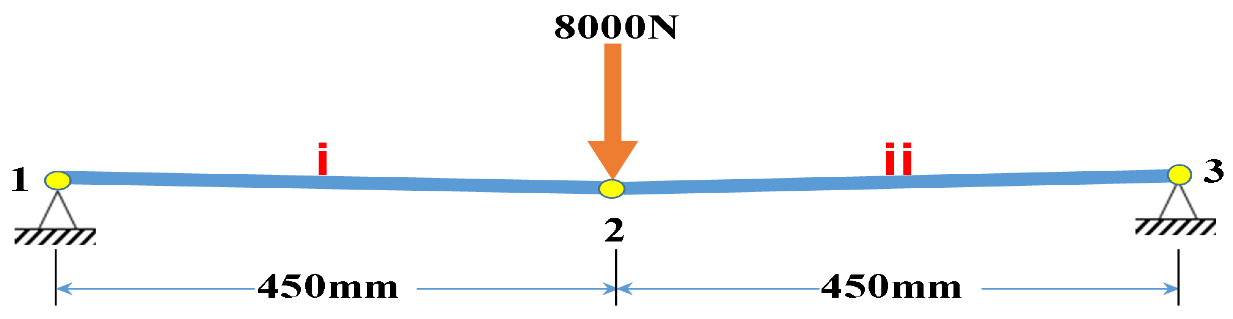
18] is based on conventional FM; it is one of the accurate methods to analyze geometrically non-linear structures. The author explicitly derived the non-linear static response to loads as presented in Equation (2), and he applied the technique through a simple two-leg structure, flat net in three-dimensional space, Saddle net, and Hyperbolic paraboloid net. The two-leg structure has also been implemented in this paper (
Figure 1). He validated the approach by Geometric Stiffness Matrix, Dynamic Relaxation, and General Minimum Energy.
in which
is the external load,
are bar modulus of elasticity and cross-sectional area,
is the bar’s initial length,
is the pretension force in the bar, and
is the joint displacement.
3. Establishing the Proposed Approach
3.1. Formulation of the Technique
The proposed algorithm is based on the stiffness matrix method [
29]. Strain can be expressed as Equation (3) through the displacement of nodes.
where
is the strain at any point,
is nodal displacement, and
is the strain displacement matrix. The statement of virtual work for a body of the volume with boundary surfaces is as follows:
Here, is the virtual displacement vector , = body force per unit volume (this often relates to the weight density), = Virtual nodal displacement, = Stress at any point, = surface load per unit area (example a pressure), = point loads, V = body of the volume, and S = boundary surfaces.
The stress in the above equations can be expressed as follows:
The stiffness of an element can be written as below.
The detailed derivation can be found in Nikishkov [
29], then the assembled stiffness matrix becomes
where
is the applied load,
is the stiffness matrix, and
is the external nodal displacement vector. Equation (7) is no longer valid for geometrically non-linear structures; hence, the proposed technique suggests that the loads should be incremented in order to obtain partial displacements such that the equation becomes
The stiffness matrix depends on the geometry of the structure, so
K is changed in each iteration due to the relocation of the coordinates after updating; therefore, the obtained displacements are added to the old coordinate to generate the new geometry.
Now a new
K is generated and Equation (8) is applied until
; then, the cumulative displacement can be found from Equation (10).
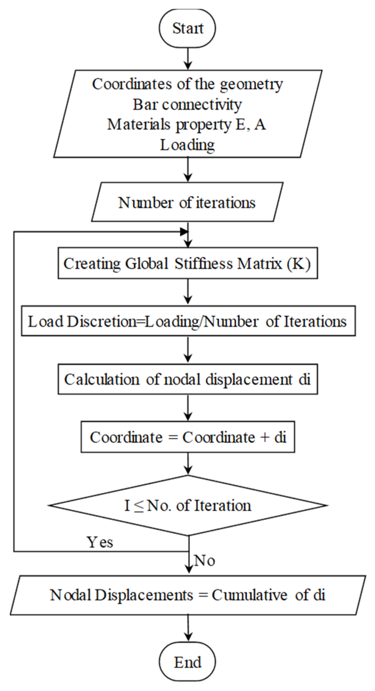
The way of working of the current technique has been illustrated in
Figure 2. The flowchart clearly explains the strategy of the work. Firstly, the geometry of the structure is entered by providing the nodal coordinates and bar connectivity. Secondly, the physical properties of the structure and the total loading are provided, and thirdly, the number of iterations is inputted. This information calculates the local and global stiffness matrix; then, load increments are manipulated. After that, the discretized load is applied, and the partial external nodal displacements are obtained. These incremented displacements are added to the former coordinates; hence, a new geometrical structure is achieved. This process is iteratively repeated until the summation of the discretized loadings is equal to the total applied load. Finally, the cumulative nodal displacements are obtained that will be the final results.
3.2. Stiffness Matrix Establishment
The stiffness matrix of a pin–pin-element based on the presented approach can be presented as follows.
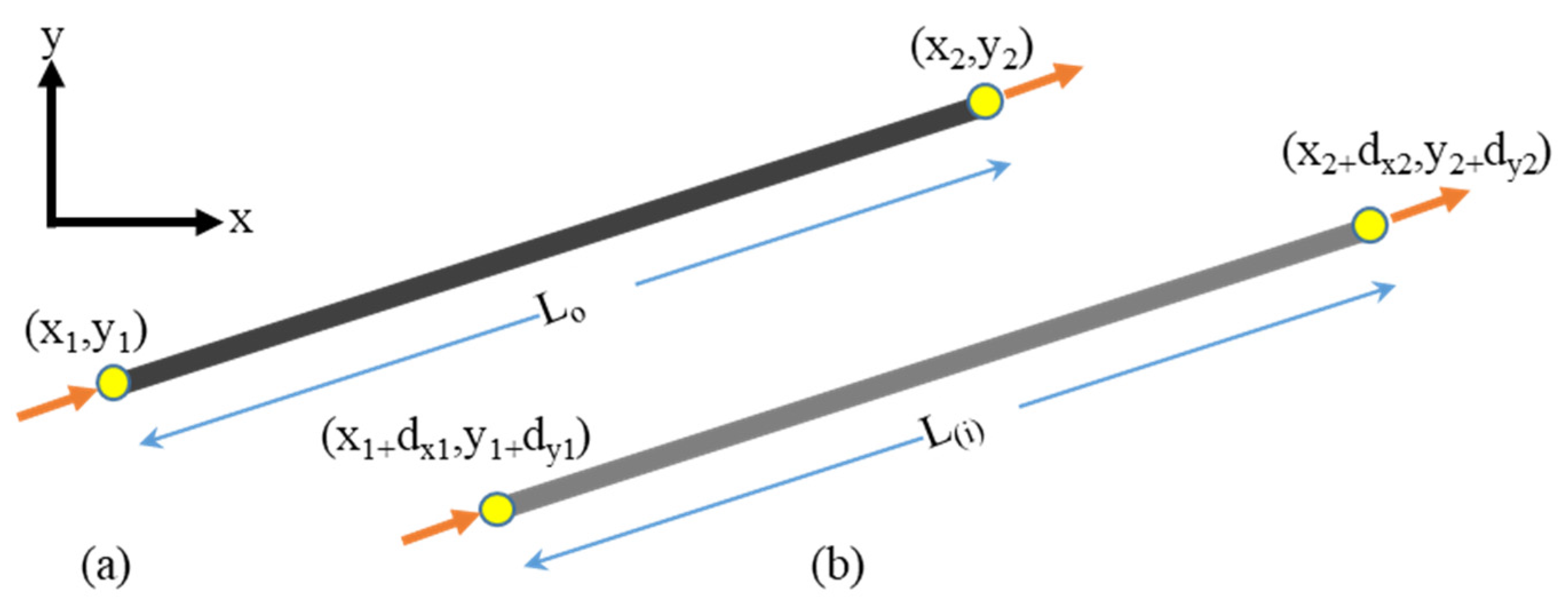
The geometry of the member before loading that shown in
Figure 3a can be found as follows:
and while , where and are the horizontal and vertical distance between the two joints of the element, respectively, while is the initial length of the member before loading. Moreover, the element stiffness matrix can be expressed as follows.
The stiffness matrix for the member before loading can be written as
where,
and
are cosine and sine of the oriented angle of the element and they can be found as
and
, respectively.
After applying Equations (3)–(9), the geometry of the element will be changed as presented in
Figure 3b and the procedure will be as follows:
and while
The stiffness matrix for member 1 can be written as
Here, and .
4. An Example for Illustrating the Technique
In this section, a simple example, which was a two-leg structure, has been tested using the current approach. The structure was supported at the two far ends; all members had
[
30], as shown in
Figure 1. The structure has been loaded at the mid joint with 8000 N downward in 15 steps sequentially (i.e., each step the structure was loaded with 8000/15 N), as shown in
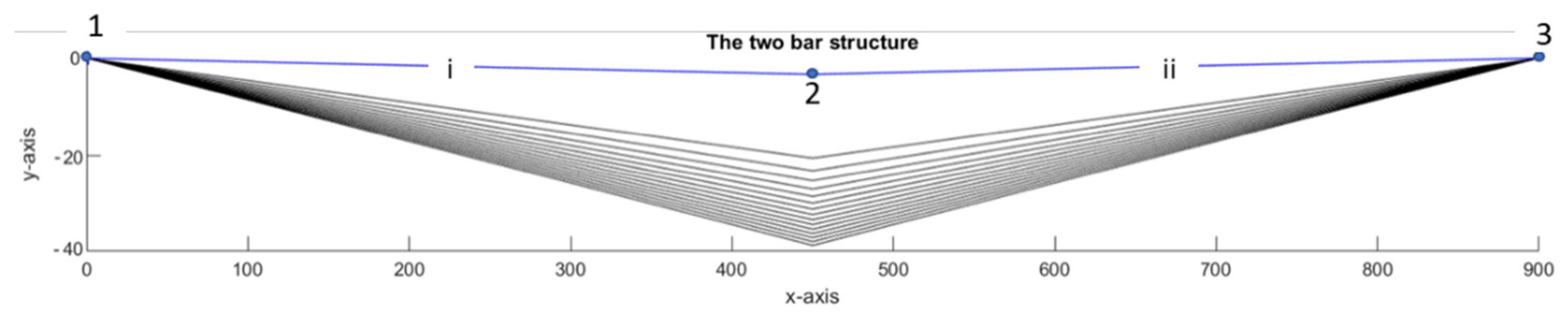
Table 1. Furthermore, the step-by-step configurations of the structure are presented in
Figure 4.
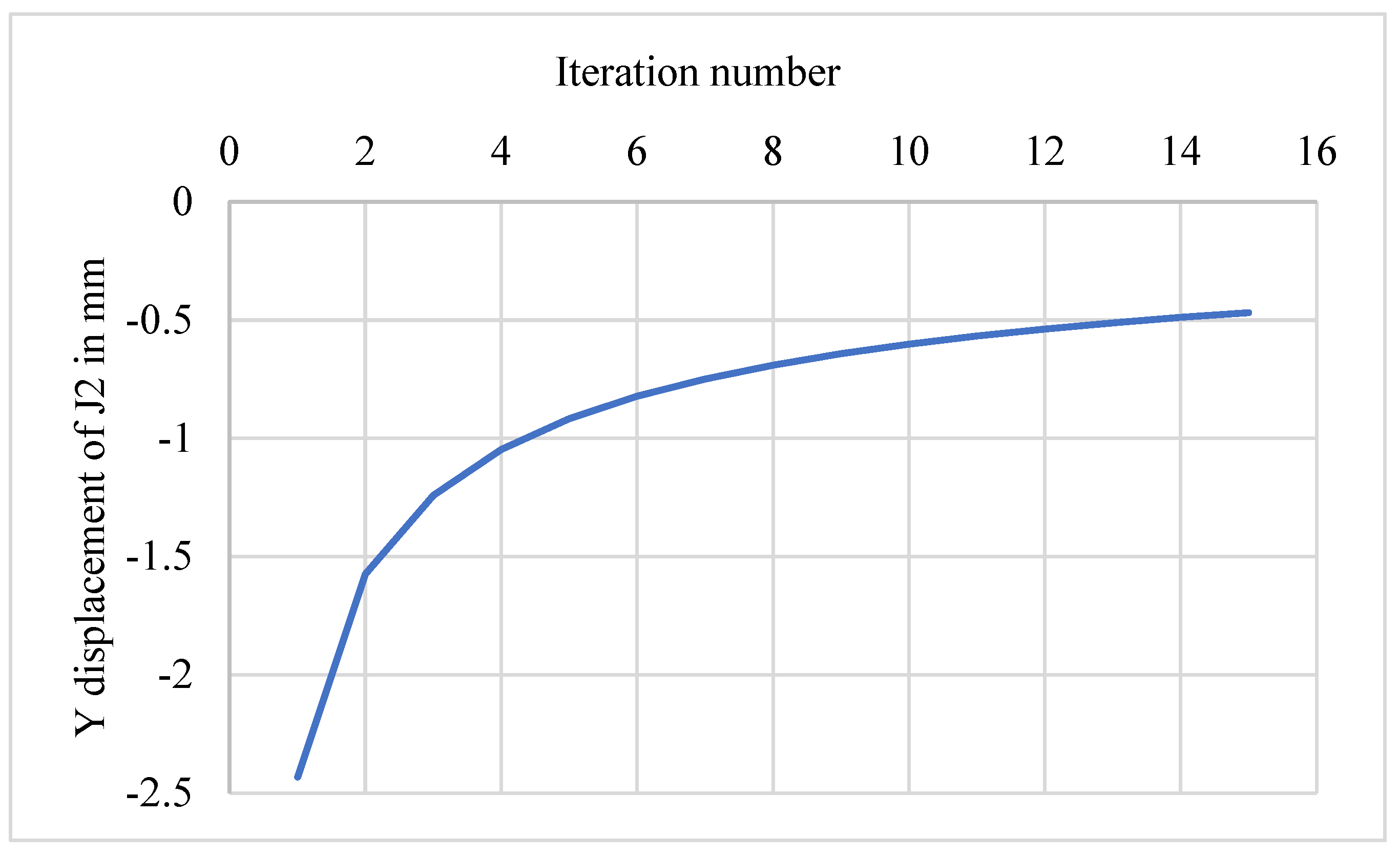
Table 1 shows the series of loading of the structure when it had different geometries. In the first iteration, the structure had the initial coordinates, and it was loaded with the first increment (8000/15 = −533.33) N. As a result, only the free joint moved downward with 2.4318 mm, then the displacement was added to the former coordinates. The change occurred only in the y-coordinate of joint 2 with the amount (10 + (2.4318)) mm; the process was continually running until the number of iterations became 15. As it is clear from
Figure 5, the amount of displacement in each step declined significantly from the first to the last iteration while the incremented loading was unchanged. This is due to the fact that the structure was stiffened by displacement [
18,
30].
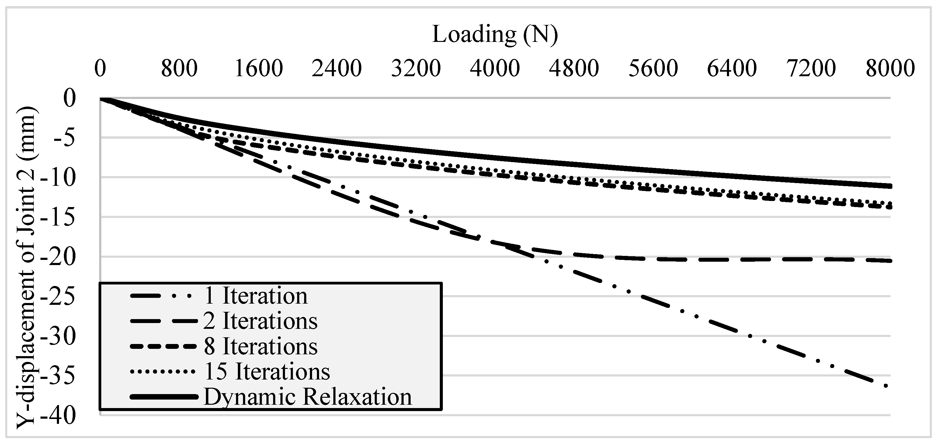
The results of different iteration numbers have been compared with conventional linear (SM), and geometrically non-linear approaches (DRM), in order to show the effect of the number of iterations on the accuracy of the method. The current approach results get closer and closer to the results from the referenced methods by increasing iteration numbers, as presented in
Figure 6. The figure clearly shows that the accuracy of the technique with respect to DRM is enhanced by increasing the number of iterations. Such that, when the number of iterations was one (i.e., when SM is applied), the end of the straight line was noticeably far from the Dynamic Relaxation curve, whereas, the curves of the results of the proposed approach got nearer to the non-linear curve by increasing the number of iterations. One can see that the most comparable curve from the solid line is the 15-iteration curve. It can be concluded that 15 iterations would be enough to get reasonable results.
5. Results and Discussion
In this section, three pin jointed structures and a cantilever beam have been tested using the current technique, conventional SM, and two quoted geometrically non-linear methods. In the following sub-sections, the results are discussed in detail.
5.1. Structure 1
The two-bar structure was tested to see the validity of the proposed technique. From this manner, the proposed approach was applied to the structure, then its displacement results were compared with the results of SM and non-linear methods.
Table 2 shows that there was a noticeable inconsistency between the displacements obtained from SM and that from geometrically non-linear methods. For this reason, it can be said that the structure behaves non-linearly.
Table 2 displays that the results of SM are significantly far from those of geometrically non-linear methods (Lewis et al., 1984; Kwan 1998), in which their discrepancy is about 228%, whereas the dissimilarity of the current study was only 16% that is reasonably close to the exact methods.
5.2. Structure 2
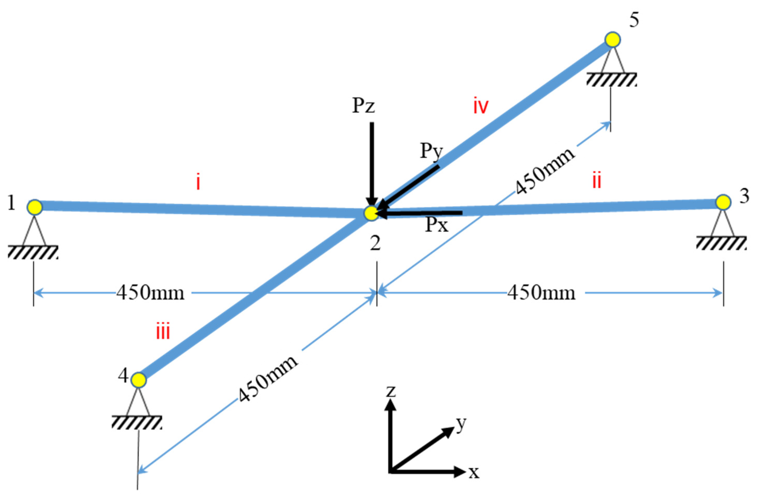
In this subsection, a 3D structure has been examined; the structure consists of four bars with four restrained joints and a free joint at the middle. The properties were the same as structure 1. However, the 3D structure has been loaded with P = 16,000 N in three directions at Joint 2, as shown in
Figure 7. It can be seen from
Table 3 that there is a negligible movement of Joint 2 in X- and Y-directions due to the response of the supports. The table also shows the validity of the proposed approach; the value of Z-direction displacement of joint 2 obtained from the current technique has a slight discrepancy with that of non-linear approaches, while the linear approach failed to get an accurate result.
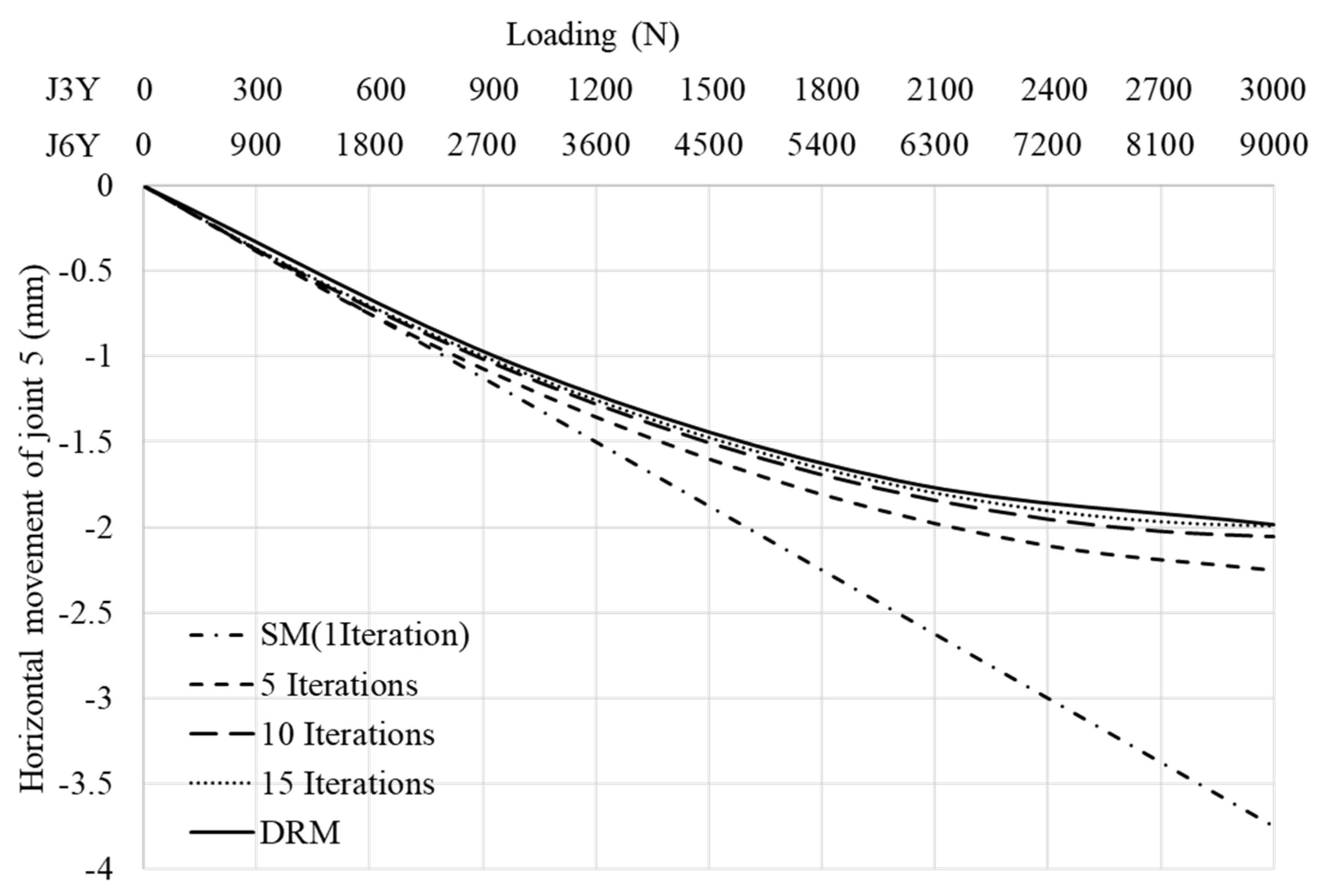
5.3. Structure 3
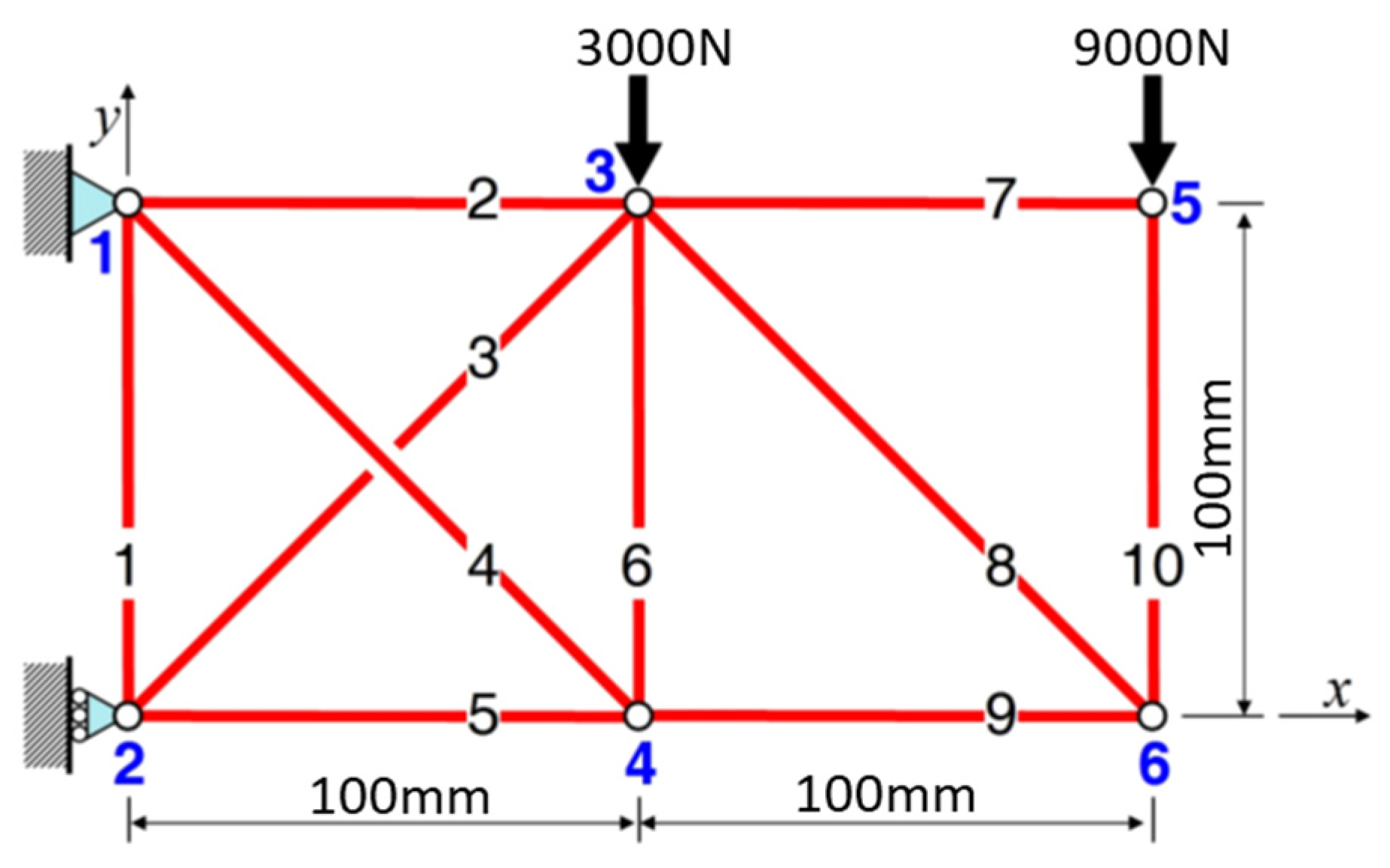
In this part, a linear pin-jointed assembly was tested, containing six joints and ten bars, as shown in
Figure 8. The bars had
. Joints 3 and 5 were loaded downward with 3000 and 9000 N, respectively, in 100 steps; the reason for applying the massive loading is to get noticeable displacement.
Table 4 gives the displacements of the two end joints (Joints 5 and 6) by the linear SM, the proposed approach and the quoted methods. The results prove that the maximum discrepancy of the referenced non-linear techniques with the proposed approach was only 5%, while the dissimilarity between non-linear techniques and the linear SM is 88%. The results demonstrate that the method is also pragmatic and accurate for linear structures with massive loading.
Furthermore,
Figure 9 clearly shows that by increasing the iteration numbers, the proposed approach results get close to the outcomes of the non-linear (DRM) method. It can be seen that from the figure, in 15 iterations, that the approach gives results reasonably close to DRM ones.
In summary, on the basis of the results of
Table 2,
Table 3 and
Table 4 of the preceding three examined structures, it can be concluded that the results of the proposed approach are in good agreement with the non-linear techniques in literature, while the results of the dependent linear technique are far from those results.
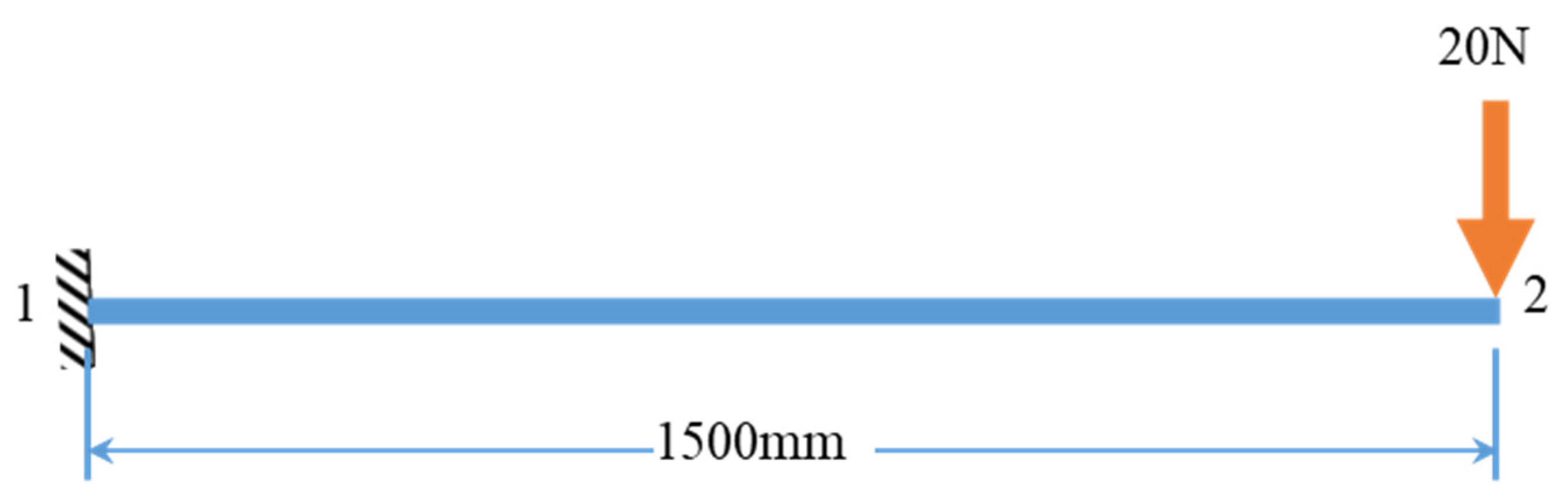
5.4. Structure 4
In this subsection, a simple cantilever beam with EI = 166.67 N.m
2, shown in
Figure 10, is examined to validate the accuracy of the current technique for analyzing geometrically non-linear flexural members. The results show that the technique is roughly in agreement with the previous non-linear technique by Lewis et al. (1984), as shown in
Table 5. It can be seen that the linear stiffness method has zero horizontal displacements, while the current approach and non-linear is clearly giving some results that are concise with the reality.
6. Conclusions
In this paper, a straightforward technique which is a partially non-linear approach has been developed from SM to analyze geometrically non-linear structures. A comparison has been made among the current technique, SM, and the two non-linear quoted methods to evaluate the accuracy of the proposed approach. The outcomes are:
- ➢
The results of the proposed technique are in good agreement with the non-linear techniques’ ones, with a slight discrepancy, while the dissimilarity between of the nodal displacements of SM and the quoted non-linear methods is 228%;
- ➢
It can be concluded that the proposed technique is accurate and applicable for geometrically non-linear structures;
- ➢
The accuracy of the technique is enhanced by increasing the number of iterations; however, the number of iterations could be assumed to be 15 to get reasonable results.


