Abstract
Before being introduced into the maintenance system, each vehicle must undergo a series of tests, including durability tests. Computer models and whole vehicles on test stands can be used to identify vehicle performance parameters, which requires access to special software and test stands. However, due to the size of the vehicle or access to test stands, experimental tests must often be carried out on proving grounds; while generating the most complete set of loads, this is much more time-consuming. Therefore, methods are sought to indicate whether testing at the proving ground can be accelerated, for example, by increasing the speed of driving or using test road sections that generate more severe loads. This paper presents a method for evaluating the suitability of selected test road sections for durability tests of a special high-mobility wheeled vehicle. The method is based on the Basquin model, which consider the fatigue strength of materials, and rainflow load cycle counting method combined with the P-M damage summation method. Evaluation of test road selection was supplemented with analysis of travel speed distributions determined using the Beta statistic distribution. The presented model was used to evaluate the ability to accelerate a mileage test of an 8 × 8 vehicle. While certain data mentioned in the article remain classified and are not able to be presented in full, the author has attempted to provide a comprehensive background of the analyses conducted and the data used to illustrate them.
1. Introduction
The exploitation environment of equipment designed for use in special conditions (e.g., forestry industry, power industry, mining industry, or the military) is changing rapidly due to, among other things, the availability of new technologies, the need to ensure higher comfort of work, and the need to meet new emission limitations. Currently-produced engineering objects are energy efficient, comfortable, relatively easy to use and eco-friendly. However, implementation of new solutions to such objects often results in higher purchase costs. Unit maintenance cost can be balanced by sufficiently efficient and failure-free operation of such objects, which is the effect of appropriate training of the operator and the suitability of the technical parameters of the object to the local conditions of use. Another way to improve efficiency ratings is to modernize existing equipment. New and modernized equipment is expected to be of consistently high quality and sufficiently long service life. This is evident in many industries, including special high-mobility wheeled vehicles designed for off-road use. With regard to vehicles manufactured in the 1970s and 1980s, their operation potential was planned for 30 years and the mileage for 200–250 thousand kilometers. However, at present, these expectations are changing in the direction of increasing the mileage to 500–600 thousand kilometers and decreasing the service life to 20 years [1]. The verification of assumptions about the maintenance profile demands appropriate changes in the field of vehicle production and in its equipment, with newer systems supporting the work of crews, e.g., [2,3,4], as well as in the testing and verification of operating parameters [5]. Invariably, great difficulties appear when evaluating the durability of such vehicles with respect to the target mileage [6,7].
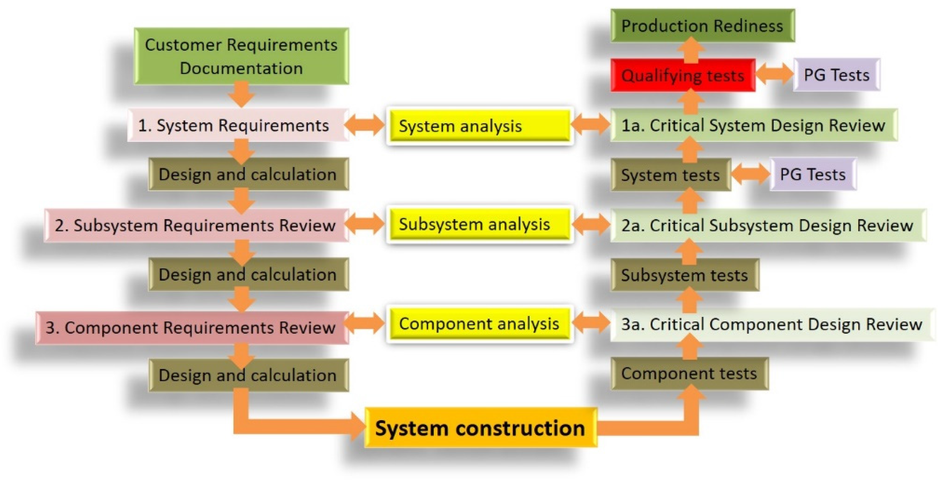
Analysis and verification of the durability of a new vehicle is carried out in several stages, most often in accordance with the adopted design model, e.g., shown in Figure 1 [8]. Three basic stages of the verification of design assumptions can be distinguished: analysis of computational models and virtual tests carried out with the use of dedicated computer software (Final Element Method—FEM, Multibody Dynamic Simulation—MBDS) [9,10]; stand tests of subassemblies and, if possible, of all vehicles [11,12]; and prototype tests of qualification mileage in normal and contract research conditions on proving grounds and test road sections [13].
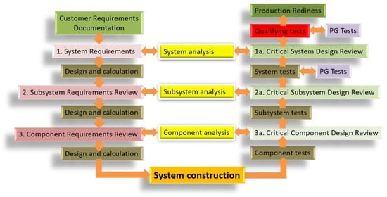
Figure 1.
A model of the system design process based on a NASA V model [8].
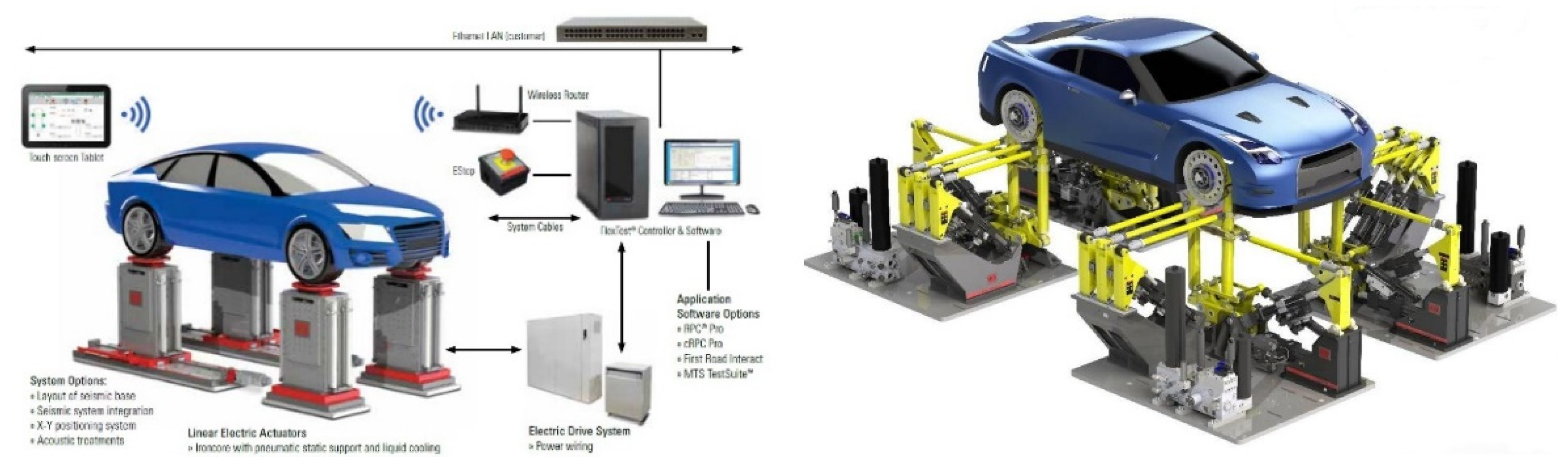
The dynamic development of computers and software has caused vehicle manufacturers to increase the share of virtual testing in the process of preparing vehicle designs for serial manufacturing, allowing for the abandonment (or limiting) of physical testing of the prototype [14]. Significant progress has been attained in the use of test rig examination of subassemblies and vehicle systems over the last 20 years, and even of whole vehicles within the last 10 years. Examples of test rigs for carrying out vehicle durability tests by generating vertical excitations from the road profile (tire-coupled road simulator) and placing the vehicle in a complex load state (spindle-coupled road simulator) are shown in Figure 2.

Figure 2.
Tire-coupled road simulator (left) and spindle-coupled road simulator (right) [11].
These tests usually concern the engine and drivetrain, steering, frame, cab, seats, suspension, hydraulics, and controls. However, the performance of such tests requires the establishment of test stand control signals (obtained by the compilation of the recorded road load data acquisition—RLDA) [5,15,16,17] and the satisfaction of the test stand requirements, which limit the possibility of testing vehicles with 6 × 6 or larger chassis and over 6000 kg GVW [11]. Moreover, such stands are very expensive; for this reason, they are used by the largest vehicle manufacturers [18]. In the case of small-series vehicle production (i.e., special vehicles) by manufacturers who often do not have extensive testing facilities at their disposal, the estimation of vehicle durability is carried out by means of experimental tests performed during test runs over a distance sufficient to observe changes and to predict the target durability of vehicle components in the context of its mileage. Here, however, a problem arises indirectly due to the high quality of the vehicle subassemblies. To observe a visible change in the durability of subassemblies as well as in the entire vehicle where bench testing of components or entire vehicles is not possible, tests under normal conditions must be performed over increasingly longer distances. Long-distance road tests of a vehicle are time-consuming and costly if only a single vehicle is available. Therefore, ways to speed up tests performed under contract research conditions, e.g., by increasing the driving speed during the tests, choosing test road sections that generate higher loads than those generated under the conditions of normal vehicle operation, and not carrying out road tests where the level of loads does not significantly limit the durability of the vehicle component being tested [15,19]. Therefore, it becomes particularly important to establish reference test road sections and running speeds for mileage tests under contract research conditions in order to establish the correlation between vehicle driving conditions (load, speed, road type) and the Remaining Useful Life (RUL) of the selected key vehicle components [20].
This paper presents a method of selection for off-road test sections in the context of generated loads at selected points of a special wheeled vehicle with 8 × 8 running gear, as well as the possibility of accelerating the tests. The method allows for determination of the model speed distributions on selected test road sections (here, off-road) and indicates which chosen off-road test sections generate the most significant loads on the key vehicle components. It is possible to estimate the possible acceleration rate of the tests in relation to the loads recorded on the reference road.
2. Vehicle Life Cycle Environmental Profile
Vehicle test conditions are specified by analyzing the stated intended vehicle operating conditions, e.g., in life cycle environmental profile (LCEP). This usually contains basic data on the operating conditions, assumed vehicle speed, cargo to be carried, and target mileage as well as indicating the types of test roads (main roads, secondary roads, off-road, cross-country) [21,22,23,24]. An example of assumptions for testing high-mobility wheeled vehicles is shown in Table 1.

Table 1.
Life Cycle Environmental Profile of High-Mobility Wheeled Vehicle (example) [23].
A more accurate analysis of predicted speeds and road types is possible based on an analysis of vehicle use conditions under operational conditions, e.g., [25,26,27]. On the basis of the data from such analyses, it is possible to arrange the test program and to select speeds and road test sections collected in a reference measurement loop for measuring loads at selected vehicle measurement points. The results of the analysis of the recorded load runs can be compared with the loads recorded on other roads of the same class to indicate the test acceleration factor, that is, the reduction in test time (h) or mileage (km).
2.1. Speed Modeling
Vehicle speed has a significant effect on the generation of loads; hence, it should be controlled in test runs. The beta statistical distribution can be used for this purpose, which allows determination of the proportions of the speed spectrum components according to the operating profile and evaluation of the speed distribution obtained from the test runs.
The statistical distribution of beta is defined as follows:
where f(x) is the percentage of the adopted speed range throughout the entire vehicle speed range, x is the value of the speed range, and A, B are the parameters of the distribution shape. Given the vehicle movement input data, for example on secondary roads (Table 1) where the assumed speed is Vavg = 50 km/h, Vmax = 80 km/h and the share of the test road section length per 1000 km of mileage is 25% (250 km), one can ascertain data to carry out the tests. This is shown in Table 2 and in Figure 3.
Table 2.
Data for Beta speed distribution (example) [27].
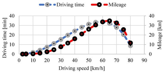
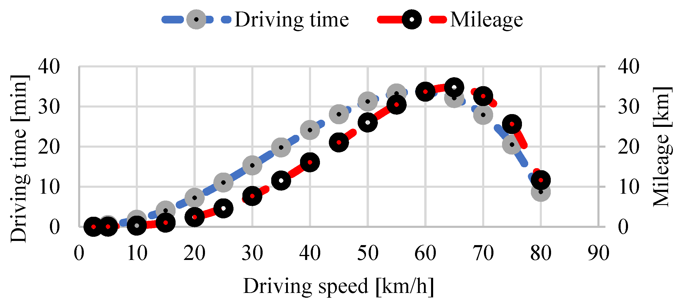
Figure 3.
Distribution of driving time and mileage as a function of driving speed (Vmax = 80 km/h; Vavg = 50 km/h; A = 3.25; B = 1.92) [27].
Small errors in determined driving time (%), i.e., 99 instead of 100, and in sectional miles (%), i.e., 102 instead of 102, are acceptable; they can be reduced by determining the A and B values more accurately. The determined speed distribution can be illustrated graphically, as shown in Figure 3.
The received speed distribution can be treated as a reference, and the determined speed distributions obtained for selected test road sections can be compared to it. Comparison of the distributions provides hints for the driver as to, e.g., whether speeds should be increased or decreased during test drives. If the given speeds cannot be reached during the measurement runs, it may be a reason to reevaluate the road section category and reclassify it (e.g., from off-road to cross-country).
2.2. Vehicle Load
According to the applicable standards and test procedures [23,24], high-mobility wheeled vehicles should be loaded with a load equal to their maximum payload during testing. This verifies the durability of the vehicle in a very conservative way. In practice, a vehicle only rarely carries a full load, especially in off-road and cross-country conditions. This has a great impact on the estimated durability, as research shows that the durability of a vehicle loaded with the maximum load compared to a vehicle without load is approximately ten times lower [28]. At the stage of selection of the test road sections, vehicle tests are carried out with the vehicle fully loaded with cargo, maintaining its correct location in the cargo space. Moreover, considering that special high-mobility wheeled vehicles are equipped with a Central Tire Inflation System (CTIS), it is important to establish and consequently maintain a constant tire pressure for the load and type of road [29]. In addition, the driving style of the driver should be monitored, e.g., by comparing the loads on the left and right sides of the vehicle to observe whether the driver is avoiding bumps under the left wheels.
2.3. Selection of Road Test Sections
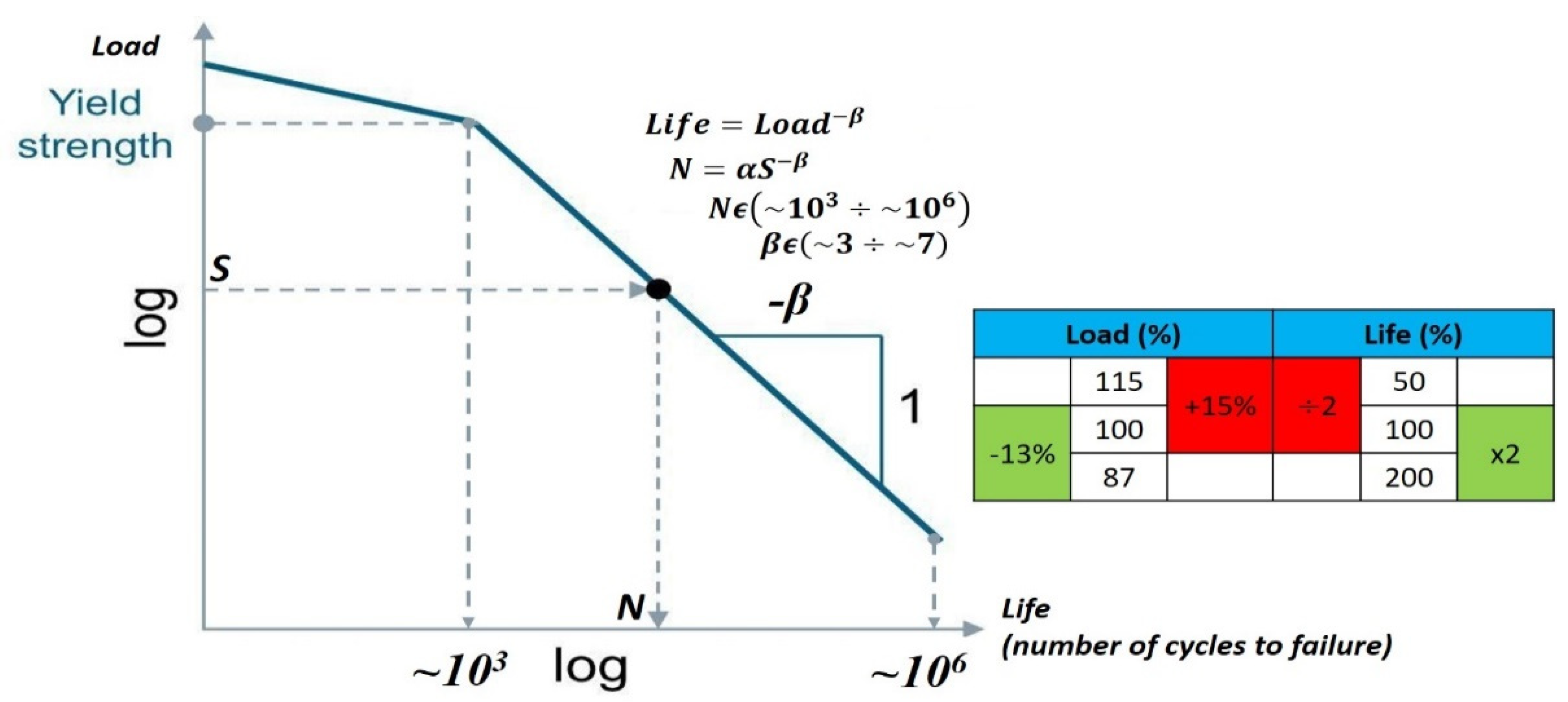
To determine whether the selected test conditions lead to the generation of greater than operating loads and to determine the possible effects of accelerated testing, an appropriate indicator is needed, with values that can be determined at the stage of qualification tests conducted by a designated testing institution when a limited set of operational data concerning the tested vehicle is available. The factor that meets these limitations may be the parameter dp, called pseudo-damage [30]. This is derived from the transformation of the general Basquin formula into the number of permissible load cycles N of monotonic loading with a range S of an element made of a material, the properties of which are represented by the coefficients α (strength of the material to the load equal to half a cycle) and β (slope coefficient of the strength curve of the material in the log-log diagram in the range of the number of load cycles N from 103 to 106) [19,31], as shown in Figure 4.
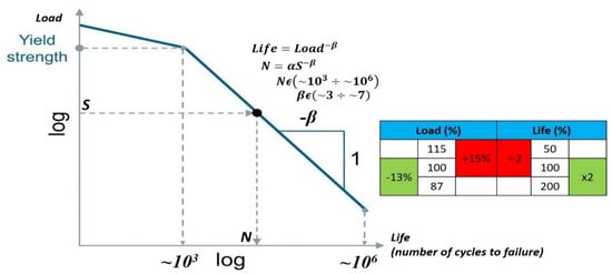
Figure 4.
Fatigue strength plot on logarithmic scale [31].
When generalizing Relation (2), the damage value can be included in the Palmgren–Miner linear damage accumulation formula as a quantity, D, which should be D ≤ 1:
Equation (3) can be expressed in a simplified form as:
where . Then, when the purpose of the tests is to compare the effect of selected operating conditions (different road sections) on the damage rate of a vehicle component, the parameters α and β can be assumed to remain constant during the tests, and Equation (4) is simplified to
where: is pseudo-damage.
It can be concluded from Relation (5) that for the evaluation of selected road sections (which have an influence on damage to the vehicle component), the load process can be recorded and then the cycles of this load can be counted using various cycle counting methods [19,32]. Taking into account the length of the road sections and assuming that the test conditions are fixed (i.e., the load, tire pressure, and speed distributions are constant), a normalized value can be determined for each road section as follows:
where is the value calculated from Relation (4) and is the length of the test section.
By performing vehicle mileage tests on various test sections of roads of the same class (e.g., off-road), it is possible to determine which road generates more damage to a component by comparing the normalized values of pseudo damage and under invariable load and comparable speed distributions in the tests:
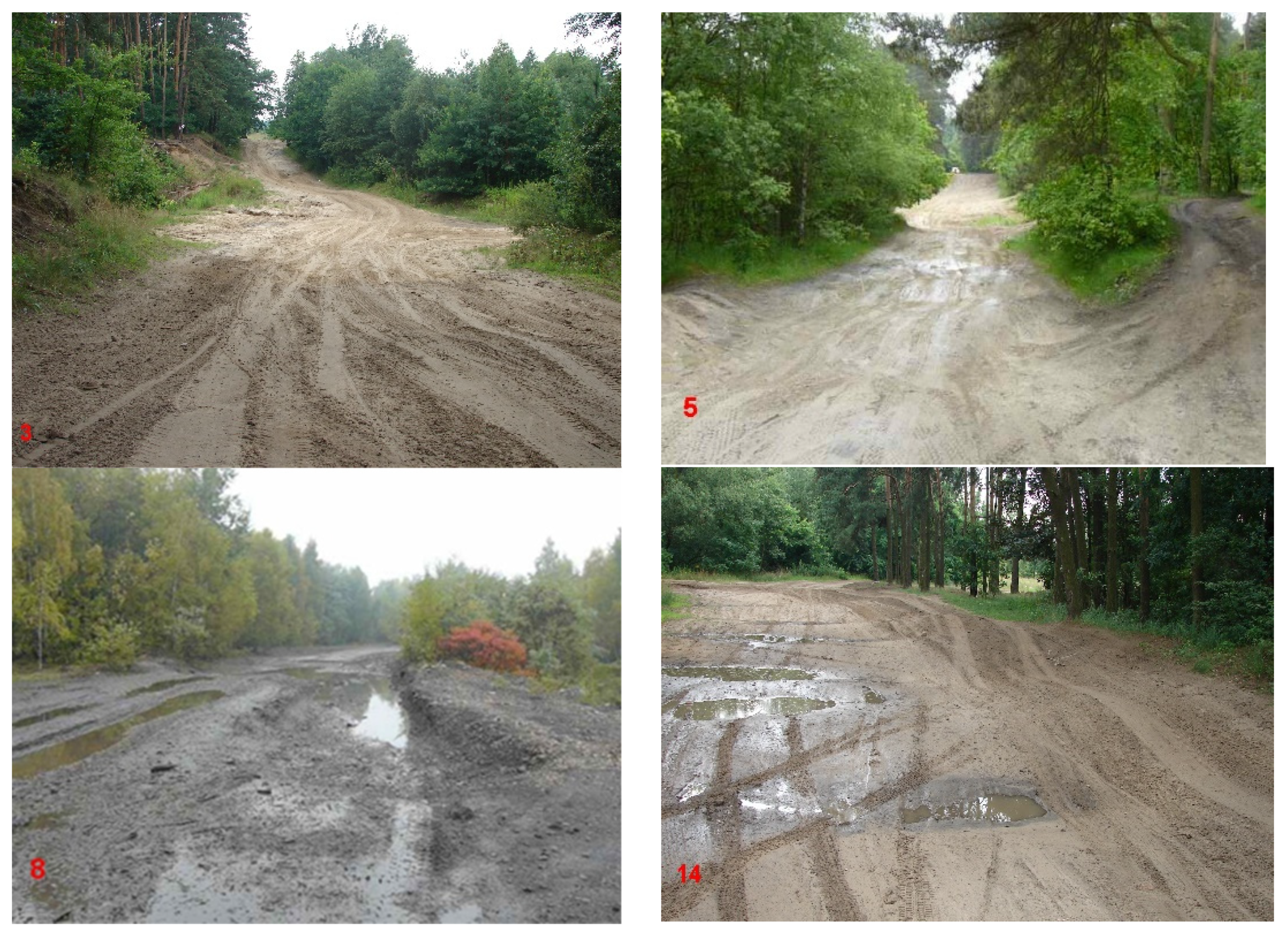
In our calculations, a preliminary value of β = 5 was assumed. This corresponds to a high cycle strength, typical for vehicle components without finishing operations such as grinding or polishing, and without notches, typical for welded joints [31]. Pictures that exemplify the analyzed test road sections are provided in Figure 5. The analyzed roads were of the off-road class only.

Figure 5.
Examples of off-road test sections (3, 5: sandy roads; 8, 14: gravel roads).
Equation (5) applies stress–strain history to determine the fatigue life of a component. For preliminary selection of test road sections, this method allows the use of other signals containing data about load cycles, for example, an acceleration signal. However, in order to obtain a direct correlation with the fatigue life of a component, the measurement data should relate directly to the stress–strain history. Then, the choice of α and β values relates strictly to the fatigue properties of the material. In other cases, the obtained value of the pseudo-damage factor dp has no reference to the fatigue strength of the material, and only indicates the fatigue nature of the forcing source (path).
3. Results
The procedure presented for the initial verification of the test road sections was carried out using a heavy-duty high-mobility wheeled vehicle. Due to the classified nature of the tests, their description and vehicle characteristics are limited. The general appearance of the vehicle is shown in Figure 6.
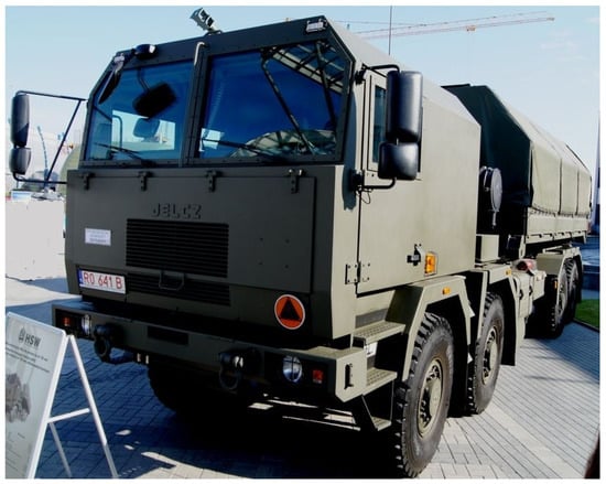
Figure 6.
General view of the tested vehicle [33].
The tested vehicle was planned for an in-service system characterized as in Table 1. Technical specifications of the vehicle are presented in Table 3.
Table 3.
Basic technical data of tested 8 × 8 vehicle.
One of the first stages of the study was to select test road sections to perform simulated in-service loads corresponding to off-road operation, which represented 55% of the target mileage. Initial research focused on finding suitable test road sections for testing suspension components. The test sections were selected for the following reasons: ability to drive at assumed speeds, load symmetry for the left and right wheel tracks, and ability to accelerate testing. The test vehicle was equipped with a measuring system that recorded the speed on each test road section and the acceleration at selected measurement points. An example presentation of speed changes on a selected test road section is provided in Figure 7.
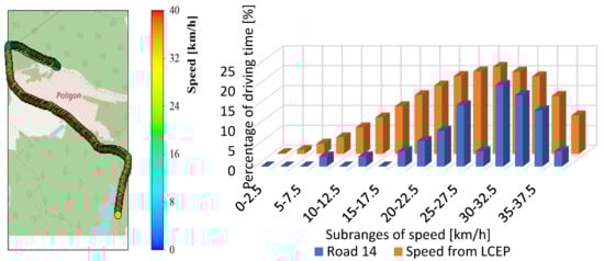
Figure 7.
Speed over Road 14 (left) and speed distribution (right).
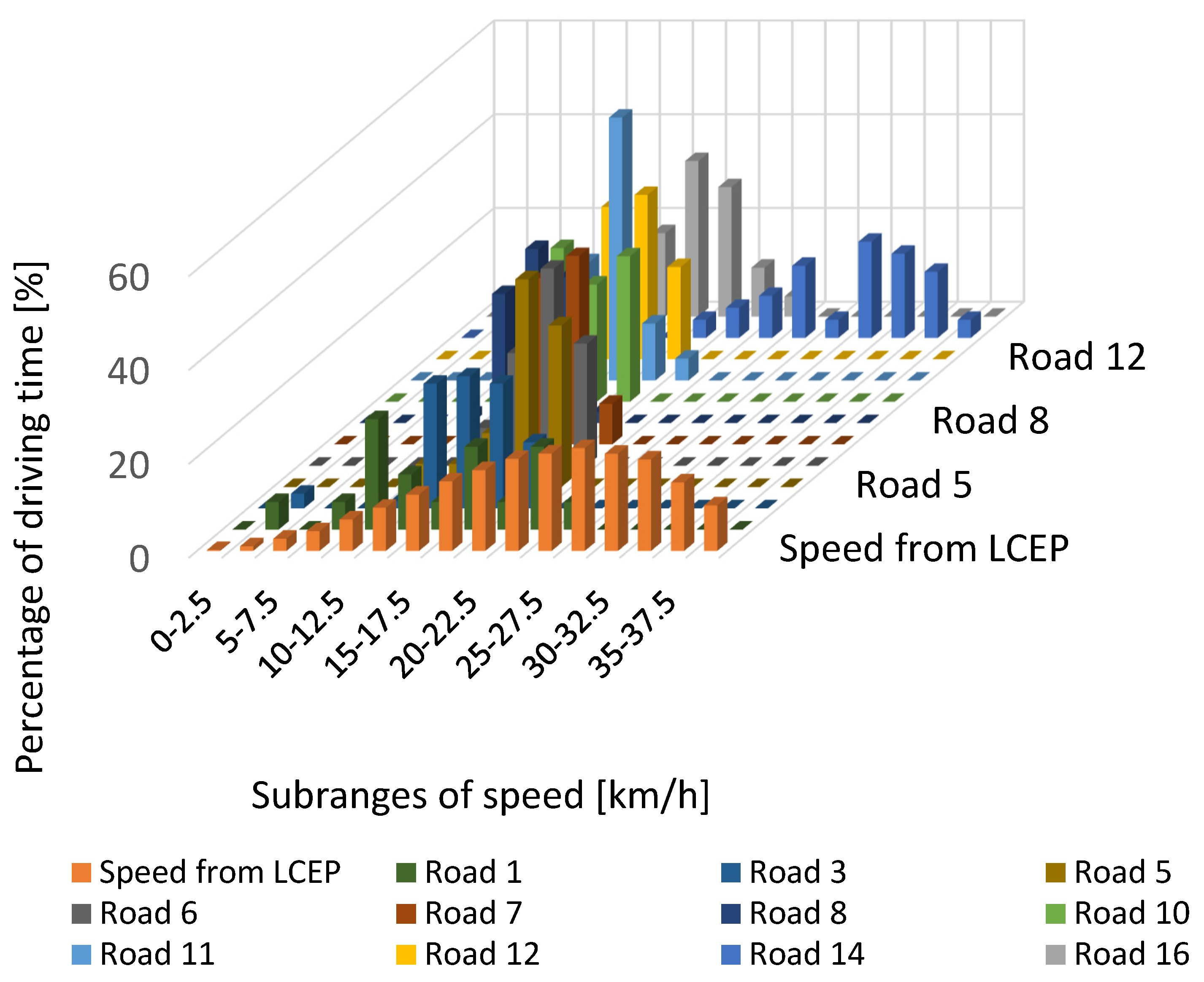
Driving speeds on selected test roads were recorded in a similar manner; speed distributions were derived from these measurements, as summarized in Figure 8.

Figure 8.
Summary of speeds on test road sections.
A summary of the driving characteristics of the selected road test sections is presented in Table 4.
Table 4.
Speeds on selected off-road class test road sections.
An example of the distribution of loads acting on the left (aL) and right (aR) sides of the vehicle is shown in Figure 9, and a summary is shown in Figure 10.
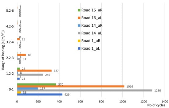
Figure 9.
Examples of cabin acceleration cycles on the left (aL) and right (aR) sides of the vehicle.
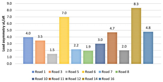
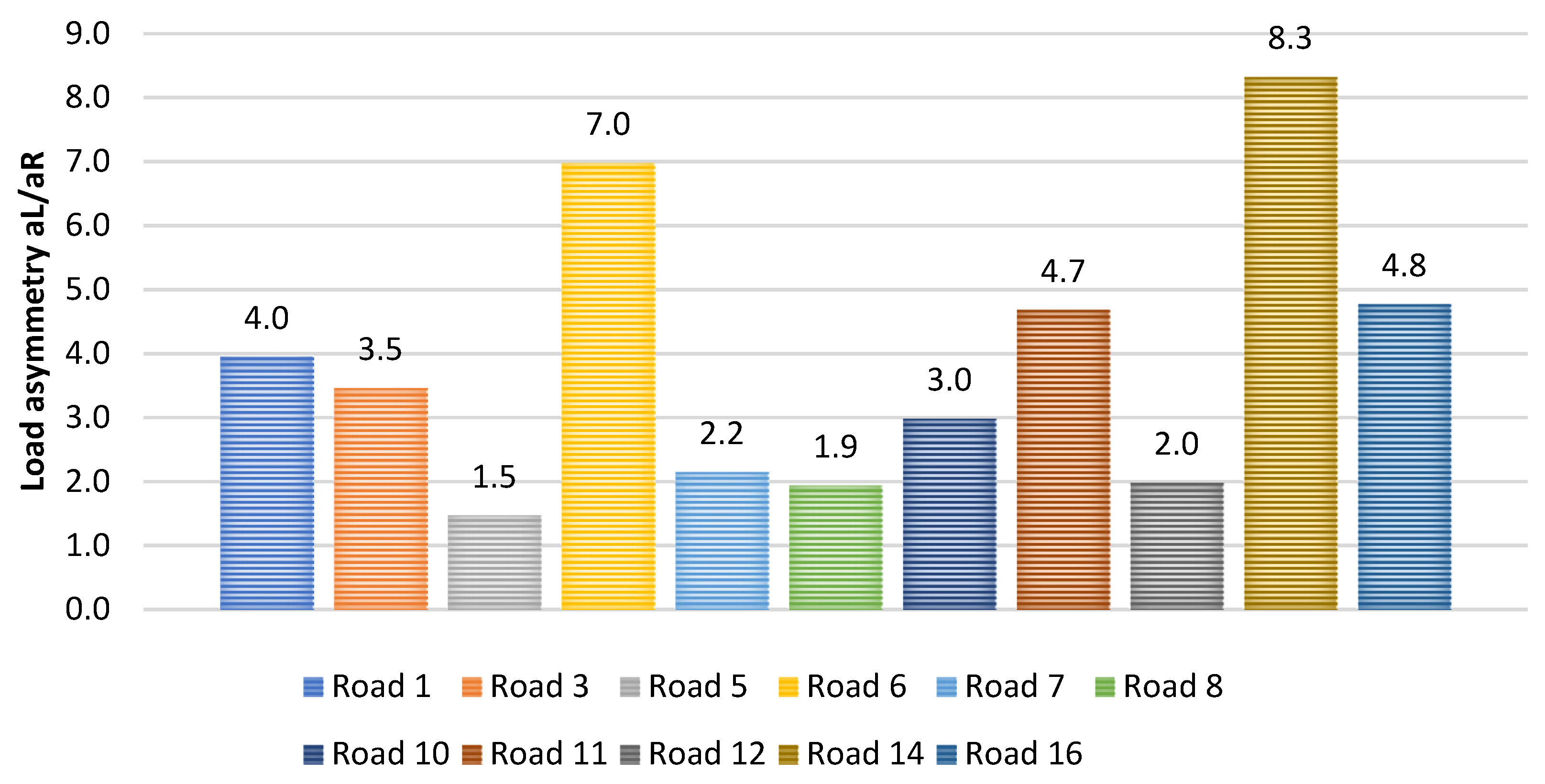
Figure 10.
Asymmetric nature of the loads acting on the wheels of the vehicle (with symmetry being dL/dR = 1).
The accelerations of the cab to the left are represented by the value aL. Respectively, the accelerations of the cab to the right side are represented by the value aR. If the acceleration distribution is balanced equally for the left and right sides, then the magnitude represented in Figure 10 as Load Asymmetry has a value of 1. If the value is greater than 1, then the accelerations operating to the left side are dominant, which may be due to larger bumps under the wheels on the right side of the vehicle.
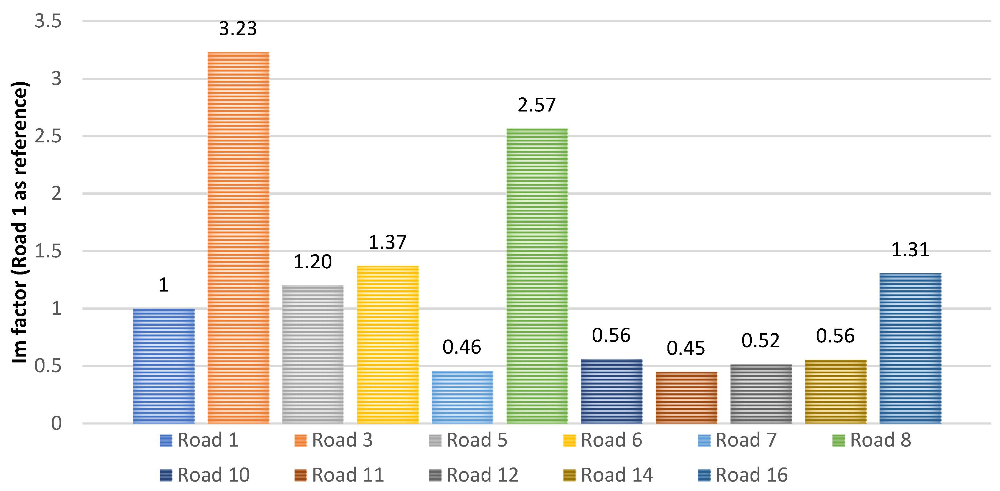
Figure 11 shows a summary of the value of the Im indicator calculated according to Equation (7), representing a multiplication of normalized loads corresponding to individual road test sections for Reference Section 1. The loads corresponded to cyclical changes in the vertical acceleration of the front axle of the vehicle which represent simultaneous deflection of the spring elements of the suspension for the left and right sides of the vehicle. This affected, among other things, the effect of the inclination of the whole vehicle around the transverse axis (i.e., pitching).
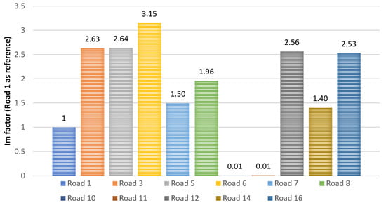
Figure 11.
Vertical loads of the unsprung mass (simultaneous deflection of parabolic springs).
Figure 12 shows a compilation of the values of the Im indicator calculated according to Equation (7), representing a multiple of the normalized loads corresponding to the individual road test sections for Reference Section 1. The loads corresponded to the cycles of change in vertical acceleration of the sprung mass on the front axle of the vehicle.

Figure 12.
Vertical loads on the vehicle frame at the front end.
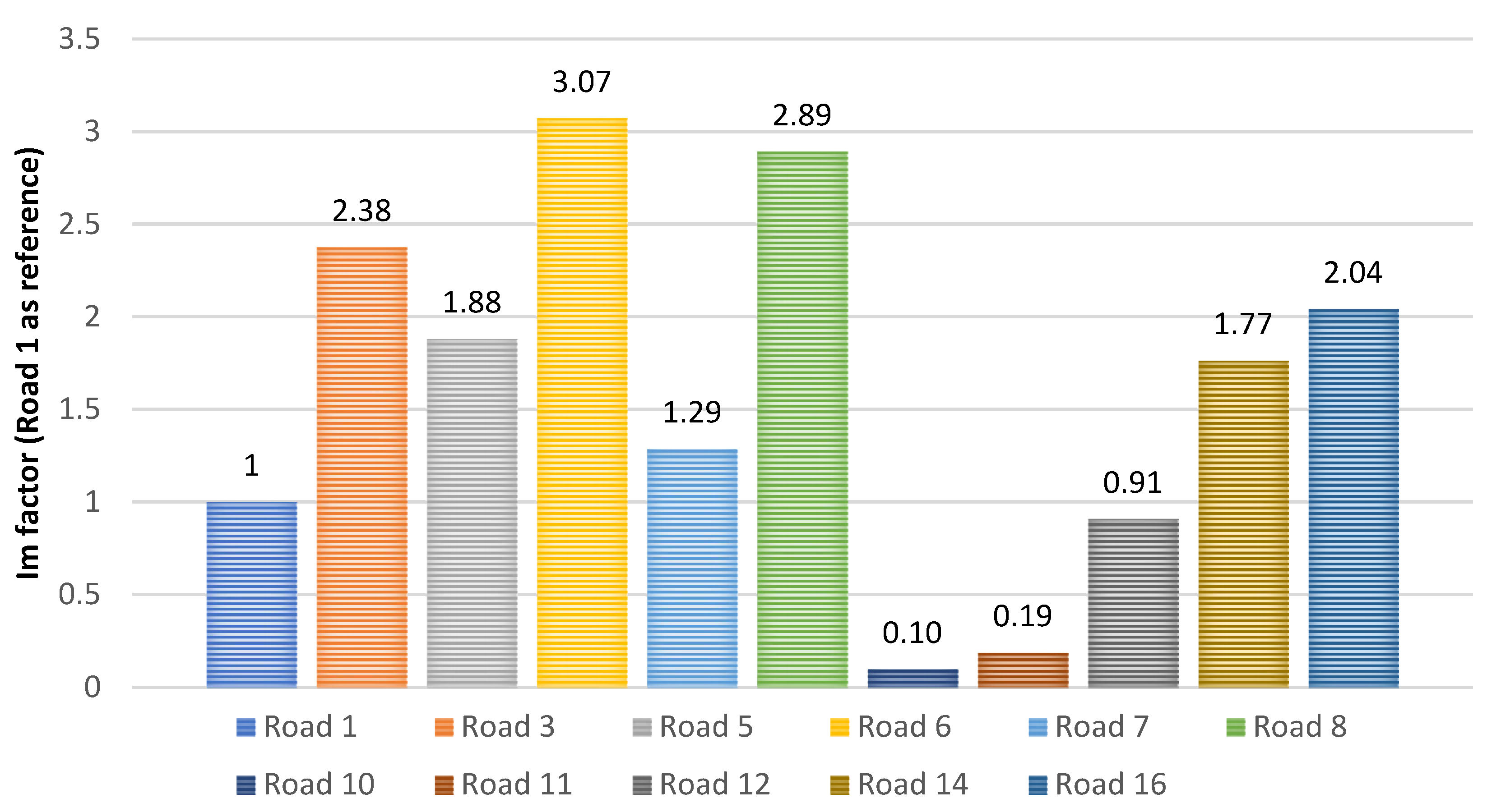
Figure 13 presents a summary of the Im indicator values calculated according to Equation (7), representing a multiple of the normalized loads corresponding to the individual road test sections with respect to Reference Section 1. The loads corresponded to cycles of changes in the angular acceleration of the front axle of the vehicle relative to the longitudinal axis of the vehicle, causing the effect of body tilting (rolling).
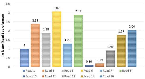
Figure 13.
Bending of the front axle stabilizer bar.
4. Discussion
The data presented in Figure 7 and Figure 8 show that vehicle speed distributions during the test run were different from the assumptions included in the LCEP; the maximum and average speeds in the road test sections were between 50% and 70% with respect to the reference speed. Both the achieved maximum and average speeds were lower compared to the required values (see Table 1). The achieved speeds were closest to the LCEP on the Test Section 14, as indicated in Table 4. The other road sections did not allow the assumed speed limits to be reached. On the basis of this, a preliminary conclusion can be made that the road roughness profile places the roads between off-road and cross-country. Due to the type of road surfaces in question, the roughness profile is not constant and may change seasonally throughout the year. This is a variable factor that should be taken into account when planning vehicle durability tests.
From the chart in Figure 9 and Figure 10, it can be seen that the loads were asymmetric during the test drives. The load asymmetry index shows a consistent pattern wherein cab accelerations to the left have values greater than accelerations to the right. In Figure 9, the results of the test of the symmetry of the loads acting on the left and right wheels of the vehicle are presented for the Test Sections 14 and 16 and the Reference Section 1. The data presented in this case provide an assessment of the load symmetry, which affects the equal load on the left and right side of the vehicle. It can be seen from this figure that there is load asymmetry in each of the assumed ranges in the sections shown. A summary of the determined asymmetry is shown in Figure 10. This may be due to different bump profiles on the left and right sides of the vehicle, to the driver’s driving style, or to a combination of those factors. An effort can be made to eliminate the effect of load asymmetry by alternating runs in opposite directions on each section of the test road. If this does not correct the observed load asymmetry, it may be improved by discussion with the driver and persuading him or her not to avoid bumps acting on the left wheels of the vehicle.
From the data presented in Figure 11, it can be seen that the highest vertical loads inducing simultaneous deflection of the left and right suspension appear on Test Sections 3, 5, 6, 12, and 14. In comparison to the loads occurring on Reference Section 1, the test acceleration on these sections is from two to three times higher. At the same time, the acceleration recorded on these test road sections do not result in an increase in the loads acting on the elements that make up the sprung mass of the front of the vehicle compared to Reference Section 1. This is advantageous because, as noted, the subject of the tests was the vehicle’s suspension system. By analyzing the data presented in Figure 13, it can be seen that Test Sections 3, 5, 6, 8, 14, and 16 caused loads that led to angular motion of the vehicle axles. At the same time, it can be observed that Test Section 12 is better-suited for testing springs than for testing stabilizers. It can additionally be pointed out that Test Sections 10 and 11 did not generate significant loads, leading to the conclusion that they can be excluded from the testing programme.
5. Conclusions
The implementation of the method presented here should begin by determining the assumed test speeds (Vmax and Vavg) from the LCEP data. Then, control spreads should be performed using the beta distribution for the preselected road section types. In the next step, the control rides should be performed and the symmetry of the loads for the left and right paths should be checked. After acceptance of the obtained results, the recording of the loads at the chosen points can be carried out and the possible Im factor can be evaluated. The further procedure depends on the specific objectives of the tests and the decisions to be made. The presented procedure for the initial selection of road test sections allows identification of the most suitable test road sections for the planned tests. The use of the Beta statistical distribution provides a reference distribution of the test speed, which is the basis for evaluating the speeds achieved on the test road sections. The use of acceleration as a load indicator is easy to use and simple to interpret. As can be seen from the presented results, when testing the springs, the highest test acceleration was achieved Test Sections 7, 8, 10, and 11 due to their high deflection values. However, in order to take into account the loads acting on the stabilizers, Test Sections 7, 8, and 14 can be eliminated from the testing programme. Considering the speed distributions on individual test road sections, it can be seen that only Test Section 14 provides speeds close to those in the LCEP; over the other sections, speeds were lower than assumed. This leads to the general conclusion that for advanced accelerated testing specially prepared test road sections should be used, as these can cause particular forms of loading and permit the possibility of significantly accelerated testing.
Funding
This research did not receive external funding. The findings presented in this paper, carried out within the framework of the research project entitled “Model of the system of load identification of the critical element of the suspension system of a high-mobility wheeled vehicle of military purpose to the requirements of Health and Usage Monitoring System—HUMS and estimation of Remaning Useful Life—RUL” granted from the pro-quality subsidy for the development of research potential of the Faculty of Mechanical Engineering PWr in the year 2022.
Institutional Review Board Statement
Not applicable.
Informed Consent Statement
Not applicable.
Data Availability Statement
The study did not report any data.
Acknowledgments
The author acknowledges that the vehicle for testing was provided by the manufacturer. The manufacturer’s representatives had no influence on the research or the final results.
Conflicts of Interest
The funders had no role in the design of the study; in the collection, analyses, or interpretation of data; in the writing of the manuscript, or in the decision to publish the results.
References
- DTU-4.22.13.1(A). Catalog of Operating Norms for Land Machinery; Ministry of Defense of Poland, Armed Forces Support Inspectorate: Bydgoszcz, Poland, 2019. (In Polish) [Google Scholar]
- GPS. Global Positioning System. Available online: https://www.gps.gov (accessed on 22 March 2022).
- C5ISR. U.S. Army Combat Capabilities Development Command (DEVCOM). Available online: https://c5isr.ccdc.army.mil/ (accessed on 1 March 2022).
- Hockley, C.J. Enterprise Management of Health and Usage Monitoring Systems (HUMS) and Condition Based Maintenance (CBM) in the UK Land Environment. In Proceedings of the “Implementation of Condition Based Maintenance”, Bucharest, Romania, 4–7 October 2010. [Google Scholar]
- MILSTD-810H. Environmental Engineering Considerations and Laboratory Tests; Department of Defense Test Method Standard: Philadelphia, PA, USA, 2019. [Google Scholar]
- Berger, C.; Eulitz, K.-G.; Heuler, P.; Kotte, K.-L.; Naundorf, H.; Scheutz, W.; Sonsino, C.M.; Wimmer, A.; Zenner, H. Betriebsfestigkeit in Germany—An overview. Int. J. Fatigue 2002, 24, 603–625. [Google Scholar] [CrossRef]
- Facchinetti, M.L. Fatigue damage of materials and structures assessed by Wöhler and Gassner frameworks: Recent insight about load spectra for the automotive. Procedia Eng. 2017, 213, 117–125. [Google Scholar] [CrossRef]
- V-Model. NASA System Engineering Handbook; NASA/SP-2016-6105 Rev2 supersedes SP-2007-6105 Rev 1 dated December; Createspace Independent Publishing Platform: Washington, DC, USA, 2017. [Google Scholar]
- SIMCENTER 3D (NX CAE); Siemens Digital Industries Software: Munich, Germany. Available online: https://trials.sw.siemens.com/nx-cam (accessed on 2 February 2022).
- ABAQUS(6.21-9); Simulia—Dassault Systemes: Vélizy-Villacoublay, France. Available online: https://www.3ds.com/products-services/simulia/products/abaqus/ (accessed on 2 February 2022).
- MTS Systems Corporation. Available online: www.mts.com/en/products (accessed on 11 February 2022).
- Instron. Available online: www.instron.com/automotive-testing-solutions (accessed on 11 February 2022).
- Norm BN-79:3615-01. Vehicle and Trailer Testing. General Guidelines; Polski Komitet Normalizacyjny: Warszawa, Poland, 1979. (In Polish) [Google Scholar]
- Volkswagen Builds Virtual Test Environment with Red Hat OpenShift. Available online: https://www.redhat.com/en/resources/volkswagen-group-case-study (accessed on 14 February 2022).
- Brudnak, M.; Walsh, J.; Baseski, I.; LaRose, B. Durability test time reduction methods. SAE Int. J. Commer. Veh. 2017, 10, 113–121. [Google Scholar] [CrossRef]
- Gao, J.; Guo, M.; Zhang, X.; Yu, X. DFD Stratagem Investigation on Suspension Subframe Durability Test with Spindle Coupled Road Test Simulator; SAE Technical Paper; SAE: Pennsylvania, PA, USA, 2020; Volume 1, pp. 992–999. [Google Scholar] [CrossRef]
- Su, H. Vibration Test Specification for Automotive Products Based on Measured Vehicle Load Data; SAE Technical Paper; SAE: Pennsylvania, PA, USA, 2006; Volume 1, pp. 571–584. [Google Scholar] [CrossRef]
- Dodds, C.; Plummer, A. Laboratory Road Simulation for Full Vehicle Testing: A Review; SAE Technical Paper; SAE: Pennsylvania, PA, USA, 2001; Volume 26, pp. 47–55. [Google Scholar] [CrossRef]
- Socie, D.; Pimpetzki, M. Modeling Variability in Service Loading Spectra. J. ASTM Int. 2004, 2, 46–56. [Google Scholar]
- Johannesson, P.; Speckert, M. Guide to Load Analysis for Durability in Vehicle Engineering; Automotive Series; Wiley & Sons: Chichester, UK, 2014; pp. 107–167. [Google Scholar]
- STANAG 4370. Environmental Testing, 3rd ed.; NATO Standardization Agency: Brussels, Belgium, 2008. [Google Scholar]
- AECTP-240. Allied Environmental Conditions and Test Publication, 1st ed.; NATO International Staff—Defence Investment Division: Bydgoszcz, Poland, 2009. [Google Scholar]
- NO-06-A106:2005. Armament and Military Equipment, General Technical Requirements, Test and Inspection Methods, Reliability Test Methods; Ministry of Defence: Bydgoszcz, Poland, 2005. [Google Scholar]
- PDNO-23-A503. Military Vehicles—Reliability Tests; Ministry of Defence of Poland: Bydgoszcz, Poland, 2017. (In Polish) [Google Scholar]
- DD-4.22. Technical Support and Security of the Polish Armed Forces; Principles of Operation, Ministry of Defense, Armed Forces Support Inspectorate: Bydgoszcz, Poland, 2017. (In Polish) [Google Scholar]
- The State of Road Safety and Actions Implemented in This Area in 2020; Secretariat of the National Road Safety Council, Ministry of Infrastructure: Warsaw, Poland, 2021. (In Polish)
- Kosobudzki, M. Speed distribution on road test sections for the need of profile ground testing of special wheeled vehicles. In Proceedings of the International Conference on Structural Dynamic, EURODYN, Athens, Greece, 23–26 November 2020; Volume 1, pp. 669–675. [Google Scholar]
- Klepka, M.; Klepka, M.; Vaclavik, J.; Chvojan, J. Fatigue life of a bus structure in normal operation and accelerated testing on special tracks. Preced. Struct. Integr. 2019, 17, 44–50. [Google Scholar]
- Tire 14.00 R 20 XZL+ TL 164/160J MI, Technical Data, Michelin. 2014. Available online: https://www.heuver.com/product/b01400020mijxzl00/14-00r20-michelin-xzl-164-160j-tl-m-s (accessed on 16 March 2022).
- Kosobudzki, M.; Smolnicki, T. Generalized vehicle durability index for different traffic conditions. AIP Conf. Proc. 2019, 2078, 020017. [Google Scholar] [CrossRef]
- Lee, Y.-L.; Pan, J.; Hathaway, R.; Barkey, M. Fatigue testing and analysis. In Theory and Practice; Elsevier Butterworth-Heinemann: Burlington, VT, USA, 2005; pp. 126–140. [Google Scholar]
- Standard Practices for Cycle Counting in Fatigue Analysis—E 1049-85; American Society for Testing and Materials, ASTM: West Conshohocken, PA, USA, 1997.
- International Defence Industry Exhibition MSPO. Available online: www.targikielce.pl/en/mspo (accessed on 16 March 2022).


Publisher’s Note: MDPI stays neutral with regard to jurisdictional claims in published maps and institutional affiliations. |
© 2022 by the author. Licensee MDPI, Basel, Switzerland. This article is an open access article distributed under the terms and conditions of the Creative Commons Attribution (CC BY) license (https://creativecommons.org/licenses/by/4.0/).