
Model Predictive Traffic Control by Bi-Level Optimization


Abstract
:1. Introduction
2. Literature Review
- -
- Control of isolated intersection,
- -
- Traffic light control with fixed time settings,
- -
- Traffic-responsive coordinated and adaptive signal control.
3. Methodology
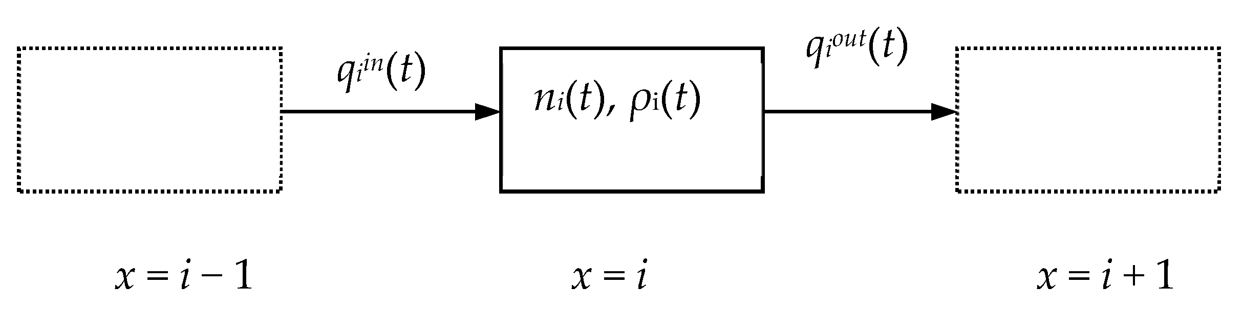
3.1. Theoretical Background of Store-and-Forward Modeling
- —input flow of the vehicles in time t, [veh/time];
- —the number of vehicles in the cell i at time t, [veh];
- —the density of the traffic flow in time t, [veh/distance].
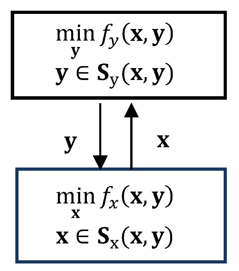
3.2. Bi-Level Formalization in Traffic Control Problems
4. Results
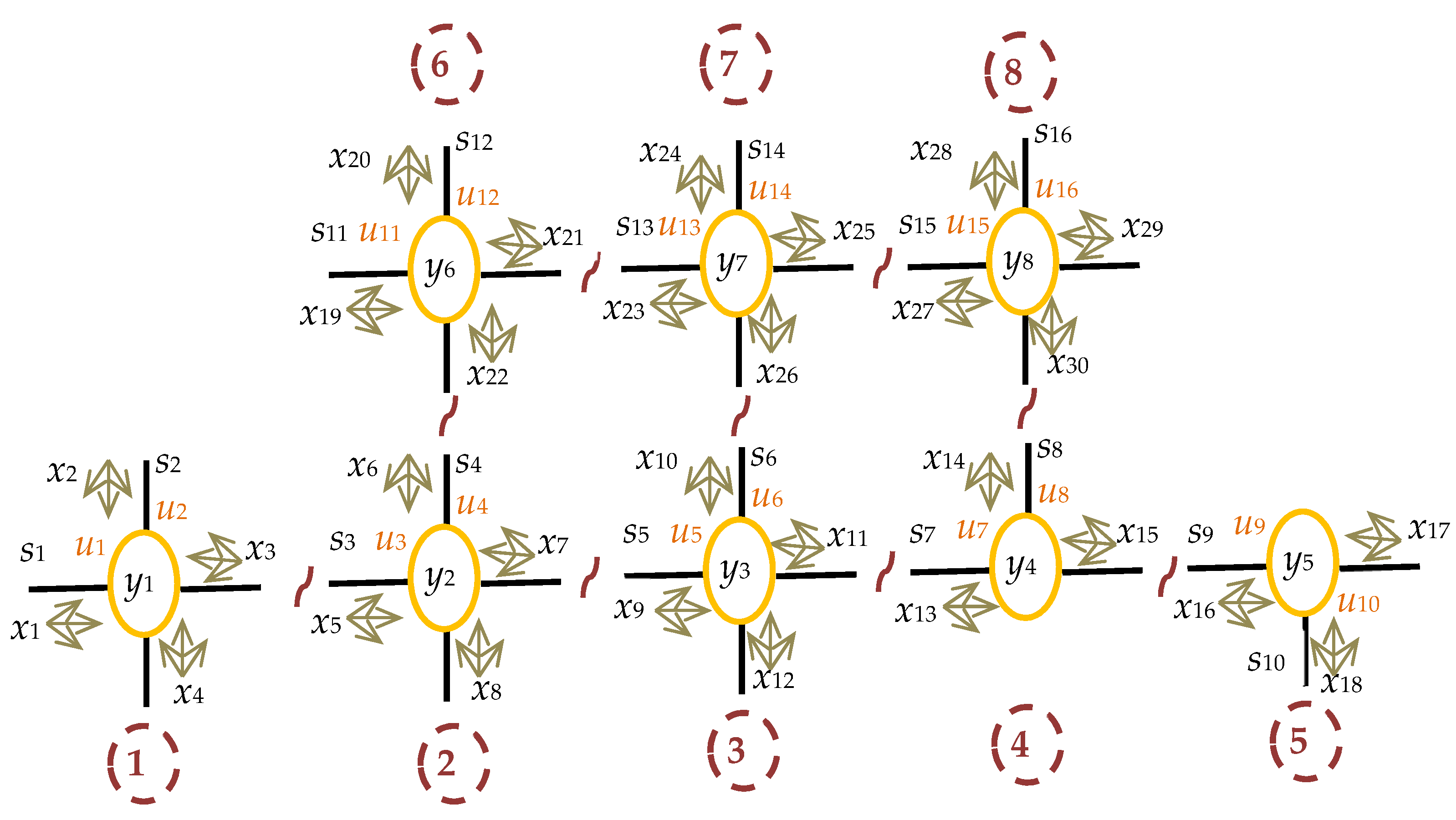
4.1. Traffic Network Topology
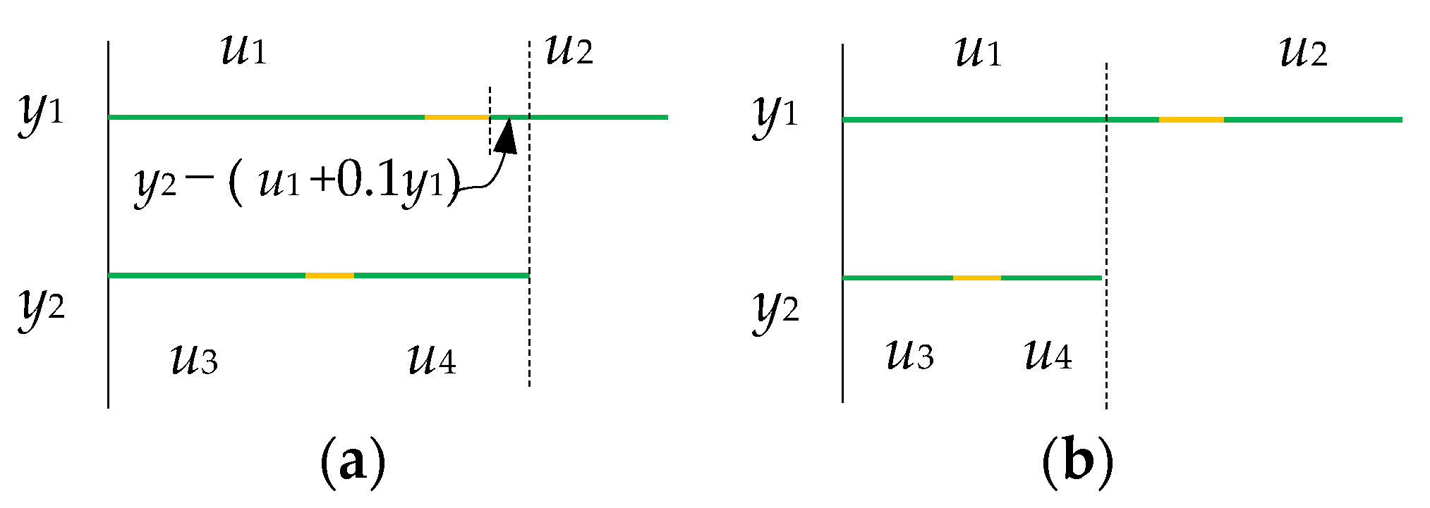
4.2. Definition of the Lower-Level Problem
4.3. Definition of the Upper-Level Problem
5. Solution of the Bi-Level Optimization Problem
6. Experiments and Results
7. Discussion and Conclusions
Author Contributions
Funding
Institutional Review Board Statement
Informed Consent Statement
Data Availability Statement
Conflicts of Interest
References
- Kachroo, P.; Özbay, K. Feedback Control Theory for Dynamic Traffic Assignment. In Advances in Industrial Control; Springer: Berlin/Heidelberg, Germany, 1999; p. 207. [Google Scholar] [CrossRef] [Green Version]
- Papageorgiou, M. Applications of Automatic Control Concepts to Traffic Flow Modeling and Control. In Lecture Notes in Control and Information Sciences; Springer: Berlin/Heidelberg, Germany, 1983; p. 190. [Google Scholar] [CrossRef]
- Childress, S. Notes on Traffic Flow. 2005. Available online: https://www.math.nyu.edu/~childres/traffic2.pdf (accessed on 1 March 2022).
- Goel, S.; Bush, S.F.; Gershenson, C. Self-Organization in Traffic Lights: Evolution of Signal Control with Advances in Sensors and Communications. 2017. Available online: https://www.researchgate.net/publication/319271996_Self-Organization_in_Traffic_Lights_Evolution_of_Signal_Control_with_Advances_in_Sensors_and_Communications (accessed on 1 March 2022).
- Luk, Y.K. Two Traffic-Responsive Area Traffic Control Methods: SCATS and SCOOT. Traffic Eng. Control 1984, 25, 14–20. [Google Scholar]
- Gartner, N.H. OPAC: A demand-responsive strategy for traffic signal control. Transp. Res. Rec. J. Transp. Res. Board 1983, 906, 75–81. Available online: https://onlinepubs.trb.org/Onlinepubs/trr/1983/906/906-012.pdf (accessed on 1 March 2022).
- Robertson, D.I.; Bretherton, R.D. Optimizing networks of traffic signals in real time-the SCOOT method. In IEEE Transactions on Vehicular Technology; IEEE: Piscataway, NJ, USA, 1991; Volume 40, pp. 11–15. [Google Scholar] [CrossRef]
- Mirchandani, P.; Wang, F.-Y. RHODES to Intelligent Transportation Systems. In IEEE Intelligent Transportation Systems; IEEE: Piscataway, NJ, USA, 2005; Volume 20, pp. 10–15. Available online: https://ieeexplore.ieee.org/stamp/stamp.jsp?tp=&arnumber=1392668 (accessed on 1 March 2022).
- Henry, J.J.; Farges, J.L.; Tuffal, J. The Prodyn Real Time Traffic Algorithm. In IFAC Proceedings Volumes; IFAC: Laxenburg, Austria, 1983; Volume 16, pp. 305–310. ISSN 1474-6670. [Google Scholar] [CrossRef]
- Mauro, V.; Di Taranto, C. Utopia. In Proceedings of the 6th IFAC/IFIP/IFORS Symposium on Control Computers and communication in Transportation, Paris, France, 19–21 September 1989; pp. 245–252. [Google Scholar]
- Diakaki, C.; Dinopoulou, V.; Aboudolas, K.; Papageorgiou, M.; Ben-Shabat, E.; Seider, E.; Leibov, A. Extensions and new applications of the traffic signal control strategy TUC. Transp. Res. Rec. 2003, 1856, 202–211. [Google Scholar] [CrossRef]
- Musabbir, S.R.; Shah, O.; Hasnat, M.M.; Haque, N. A new stochastic macroscopic model for heterogeneous traffic considering variable fundamental diagram. In Proceedings of the Transportation Research Board 95th Annual Meeting, Washington, DC, USA, 10–12 January 2016; Available online: https://www.academia.edu/16768469/A_NEW_STOCHASTIC_MACROSCOPIC_MODEL_FOR_HETEROGENEOUS_TRAFFIC_CONSIDERING_VARIABLE_FUNDAMENTAL_DIAGRAM (accessed on 1 March 2022).
- Galvan-Correa, R.; Olguin-Carbajal, M.; Herrera-Lozada, J.C.; Sandoval-Gutierrez, J.; Serrano-Talamantes, J.F.; Cadena-Martinez, R.; Aquino-Ruíz, C. Micro Artificial Immune System for Traffic Light Control. Appl. Sci. 2020, 10, 7933. [Google Scholar] [CrossRef]
- Olayode, I.O.; Tartibu, L.K.; Okwu, M.O.; Ukaegbu, U.F. Development of a Hybrid Artificial Neural Network-Particle Swarm Optimization Model for the Modelling of Traffic Flow of Vehicles at Signalized Road Intersections. Appl. Sci. 2021, 11, 8387. [Google Scholar] [CrossRef]
- Adacher, L. A global optimization approach to solve the traffic signal synchronization problem. Proced. Soc. Behav. Sci. 2012, 54, 1270–1277. [Google Scholar] [CrossRef]
- Li, Y.; Yu, L.; Tao, S.; Chen, K. Multi-objective optimization of traffic signal timing for oversaturated intersection. Math. Probl. Eng. 2013, 2013, 182643. [Google Scholar] [CrossRef]
- Lee, S.; Wong, S.C.; Varaiya, P. Group-based hierarchical adaptive traffic-signal control part I: Formulation. Transp. Res. Part B. Methodol. 2017, 105, 1–18. [Google Scholar] [CrossRef] [Green Version]
- Eom, M.; Kim, B.I. The traffic signal control problem for intersections: A review. Eur. Transp. Res. Rev. 2020, 12, 50. [Google Scholar] [CrossRef]
- Sacone, S.; Siri, S. Event-triggered model predictive schemes for freeway traffic control. Transp. Res. C 2015, 58, 554–567. Available online: https://www.academia.edu/12028241/Event_triggered_model_predictive_schemes_for_freeway_traffic_control?email_work_card=title (accessed on 1 March 2022).
- Gazis, D.C. Traffic Flow and Control: Theory and Applications: The Car Increases Man’s Mobility, until All Decide to Exercise This Mobility Simultaneously in Space and Time; Then We Must Call Traffic Science to the Rescue. Am. Sci. 1972, 60, 414–424. [Google Scholar]
- Aboudolas, K.; Papageorgiou, M.; Kosmatopoulos, E. Store-and-forward based methods for the signal control problem in large-scale congested urban road networks. Transp. Res. Part C. Emerging Technol. 2009, 17, 163–174. [Google Scholar] [CrossRef] [Green Version]
- Papamichail, I.; Kampitaki, K.; Papageorgiou, M.; Messmer, A. Integrated Ramp Metering and Variable Speed Limit Control of Motorway Traffic Flow. IFAC Proc. Vol. 2008, 41, 14084–14089. [Google Scholar] [CrossRef] [Green Version]
- Pedroso, L.; Batista, P. Decentralized store-and-forward based strategies for the signal control problem in large-scale congested urban road networks. Transp. Res. Part C. Emerging Technol. 2021, 132, 103412. [Google Scholar] [CrossRef]
- Grandinetti, P.; De Wit, C.C.; Garin, F. Distributed Optimal Traffic Lights Design for Large-Scale Urban Networks. In IEEE Transactions on Control Systems Technology; IEEE: Piscataway, NJ, USA, 2019; Volume 27, pp. 950–963. Available online: https://hal.inria.fr/hal-01727937 (accessed on 1 March 2022).
- Majid, H.; Hajiahmadi, R.; De Schutter, B.; Abouaissa, H.; Daniel, J. Distributed model predictive control of freeway traffic networks: A serial partially cooperative approach. In Proceedings of the 17th IEEE International Conference on Intelligent Transportation Systems, Qingdao, China, 8–11 October 2014; pp. 1876–1881. [Google Scholar]
- Warberg, A.; Larsen, J.; Jørgensen, R.M. Green Wave Traffic Optimization—A Survey. Available online: https://orbit.dtu.dk/en/publications/green-wave-traffic-optimization-a-survey (accessed on 1 March 2022).
- Xu, H.; Zhuo, Z.; Chen, J.; Fang, X. Traffic signal coordination control along oversaturated two-way arterials. J. Comp. Sci. 2020, 6, e319. [Google Scholar] [CrossRef]
- Lin, S.; De Schutter, B.; Xi, Y.; Hellendoorn, J. A simplified macroscopic urban traffic network model for model-based predictive control. In Proceedings of the 12th IFAC Symposium on Transportation Systems, Redondo Beach, CA, USA, 2–4 September 2009; pp. 286–291. Available online: https://www.dcsc.tudelft.nl/~bdeschutter/pub/rep/09_028.pdf (accessed on 1 March 2022).
- Wei, H.; Zheng, G.; Gayah, V.; Li, Z. A Survey on Traffic Signal Control Methods. 2020. Available online: https://arxiv.org/abs/1904.08117v3 (accessed on 1 March 2022).
- Ye, B.-L.; Wu, W.; Gao, H.; Lu, Y.; Cao, Q.; Zhu, L. Stochastic Model Predictive Control for Urban Traffic Networks. Appl. Sci. 2017, 7, 588. [Google Scholar] [CrossRef] [Green Version]
- Stoilova, K.; Stoilov, T. Integrated management of transportation by bi-level optimization. In Proceedings of the International Conference Automatics and Informatic—ICAI, Varna, Bulgaria, 1–3 October 2020; ISBN 978-1-7281-9308-3. [Google Scholar] [CrossRef]
- García-Nieto, J.; Olivera, A.; Alba, E. Optimal Cycle Program of Traffic Lights with Particle Swarm Optimization. IEEE Trans. Evolut. Comput. 2013, 17, 823–839. [Google Scholar] [CrossRef] [Green Version]
- Wu, Y.; Lu, J.; Chen, H.; Yang, H. Development of an Optimization Traffic Signal Cycle Length Model for Signalized Intersections in China. In Mathematical Problems in Engineering; Hindawi Publishing Corporation: London, UK, 2015; Volume 2015, 9p. [Google Scholar] [CrossRef] [Green Version]
- Daganzo, C. The Cell Transmission Model. Part I: A Simple Dynamic Representation of Highway Traffic. UC Berkeley: California Partners for Advanced Transportation Technology. 1992. Available online: https://escholarship.org/uc/item/0b6612tk (accessed on 1 March 2022).
- Daganzo, C. The cell transmission model: A dynamic representation of highway traffic consistent with the hydrodynamic theory. Transp. Res. Part B Methodol. 1994, 28, 269–287. [Google Scholar] [CrossRef]
- Daganzo, C. The cell transmission model, part II: Network traffic. Transp. Res. Part B Methodol. 1995, 29, 79–93. [Google Scholar] [CrossRef]
- Daganzo, C.F. On the Variational Theory of Traffic Flow: Well-Posedness, Duality and Applications. 2006. Available online: https://escholarship.org/uc/item/61v1r1qq (accessed on 1 March 2022).
- Lighthill, M.J.; Whitham, G.B. On Kinematic Waves: I: Flow Movement in Long Rivers, II: A Theory of Traffic Flow on Long Crowded Roads. Proc. R. Soc. Lond. 1955, A229, 317–345. [Google Scholar]
- Richards, P.I. Shock Waves on the Highway. Operat. Res. 1956, 4, 42–57. [Google Scholar] [CrossRef]
- Djukic, T.; Masip, D.; Breen, M.; Casas, J. Modified bi-level optimization framework for dynamic OD demand estimation in the congested networks. In Proceedings of the Australasian Transport Research Forum, Auckland, New Zealand, 27–29 November 2017; pp. 1–15. Available online: https://www.australasiantransportresearchforum.org.au/sites/default/files/ATRF2017_055.pdf (accessed on 1 March 2022).
- Bakibillah, A.S.M.; Kamal, M.A.S.; Tan, C.P.; Susilawati, S.; Hayakawa, T.; Imura, J.-I. Bi-Level Coordinated Merging of Connected and Automated Vehicles at Roundabouts. Sensors 2021, 21, 6533. [Google Scholar] [CrossRef] [PubMed]
- Li, D.; Song, Y.; Chen, O. Bilevel Programming for Traffic Signal Coordinated Control considering Pedestrian Crossing. Hindawi. J. Adv. Transp. 2020, 3987591, 18. Available online: https://www.hindawi.com/journals/jat/2020/3987591 (accessed on 1 March 2022). [CrossRef]
- Londonoa, G.; Lozano, A. A bilevel optimization program with equilibrium constraints for an urban network dependent on time. Transp. Res. Proc. 2014, 3, 905–914. [Google Scholar] [CrossRef] [Green Version]
- Sun, D.; Rahim, F.; Benekohal, R.F.; Waller, S.T. Bi-level Programming Formulation and Heuristic Solution Approach for Dynamic Traffic Signal Optimization. Comput. Aided Civil Infrastruct. Eng. 2006, 21, 321–333. [Google Scholar] [CrossRef]
- Wang, D.; Zhou, L.; Zhang, H.; Liang, X. A Bi-Level Model for Green Freight Transportation Pricing Strategy Considering Enterprise Profit and Carbon Emissions. Sustainability 2021, 13, 6514. [Google Scholar] [CrossRef]
- Sinha, A.; Malo, P.; Deb, K. Transportation policy formulation as a multi-objective bi-level optimization problem. In IEEE Congress on Evolutionary Computation (CEC); IEEE: Piscataway, NJ, USA, 2015; pp. 1651–1658. [Google Scholar] [CrossRef]
- García-Ródenas, R.; López-García, M.L.; Sánchez-Rico, M.T.; López-Gómez, J.A. A bilevel approach to enhance prefixed traffic signal optimization. Eng. Appl. Artific. Intell. 2019, 84, 51–65. [Google Scholar] [CrossRef]
- Chiou, S.W. A bi-objective bi-level signal control policy for transport of hazardous materials in urban road networks. J. Transp. Res. Part D Transp. Environ. 2016, 42, 16–44. [Google Scholar] [CrossRef]
- Holkar, K.S.; Waghmare, M. An Overview of Model Predictive Control. Int. J. Control Automat. 2010, 3, 47–63. Available online: https://www.academia.edu/11852005/An_Overview_of_Model_Predictive_Control (accessed on 1 March 2022).
- Jafari, S.; Shahbazi, Z.; Byun, Y.-C. Designing the Controller-Based Urban Traffic Evaluation and Prediction Using Model Predictive Approach. Appl. Sci. 2022, 12, 1992. [Google Scholar] [CrossRef]
- Available online: https://yalmip.github.io/command/solvebilevel/ (accessed on 1 March 2022).


| 1 | 2 | 3 | 4 | 5 | 6 | 7 | 8 | 9 | 10 | 11 | 12 | 13 | 14 | 15 | |
|---|---|---|---|---|---|---|---|---|---|---|---|---|---|---|---|
| y1 | 40 | 40 | 40 | 40 | 40 | 40 | 40 | 40 | 40 | 40 | 40 | 40 | 40 | 40 | 40 |
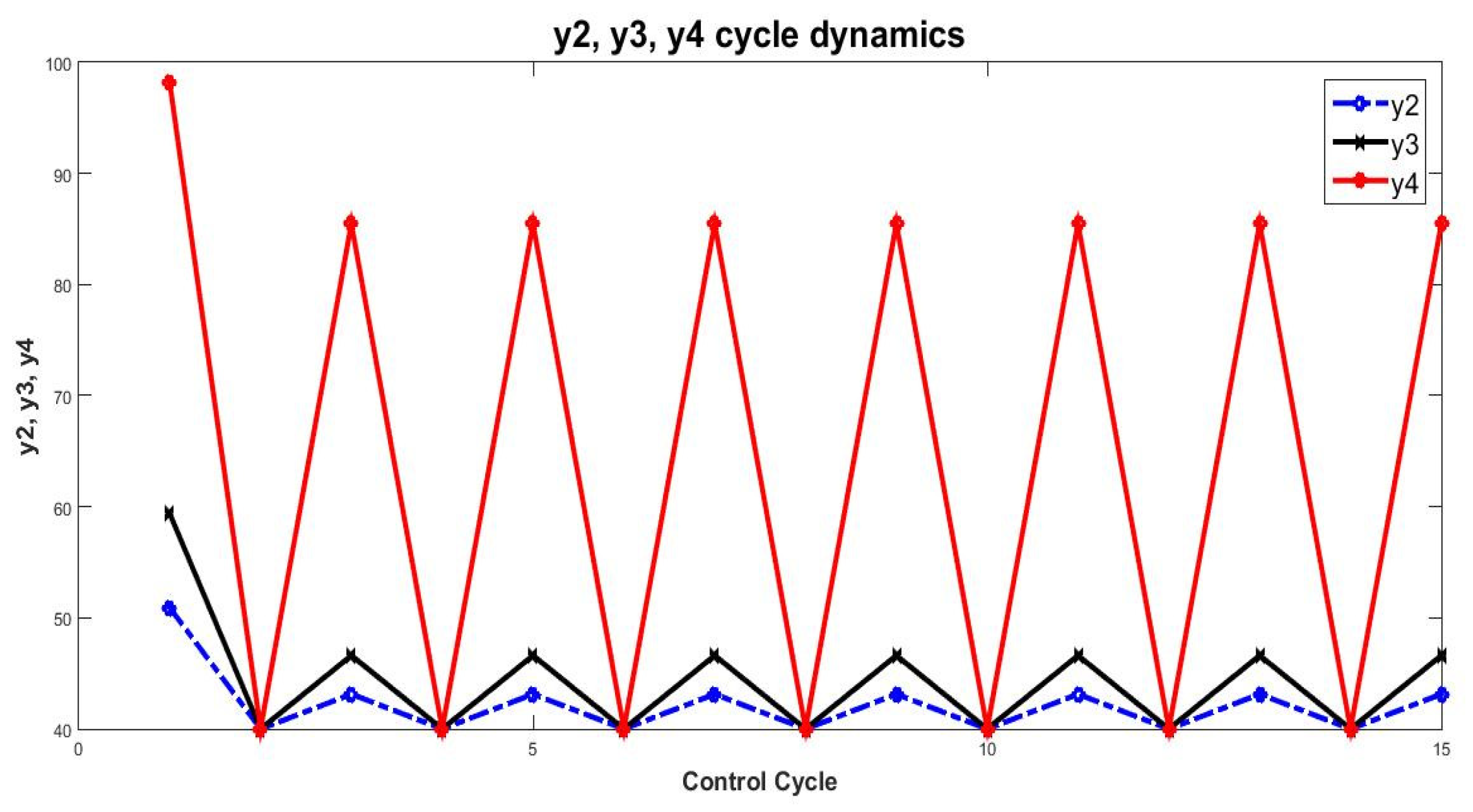
| y2 | 50.91 | 40 | 43.13 | 40 | 43.13 | 40 | 43.13 | 40 | 43.13 | 40 | 43.13 | 40 | 43.13 | 40 | 43.13 |
| y3 | 59.38 | 40 | 46.61 | 40 | 46.61 | 40 | 46.61 | 40 | 46.61 | 40 | 46.61 | 40 | 46.61 | 40 | 46.61 |
| y4 | 98.17 | 40 | 85.48 | 40 | 85.48 | 40 | 85.48 | 40 | 85.48 | 40 | 85.48 | 40 | 85.48 | 40 | 85.48 |
| y5 | 40 | 40 | 40 | 40 | 40 | 40 | 40 | 40 | 40 | 40 | 40 | 40 | 40 | 40 | 40 |
| y6 | 40 | 40 | 40 | 40 | 40 | 40 | 40 | 40 | 40 | 40 | 40 | 40 | 40 | 40 | 40 |
| y7 | 60.14 | 40 | 47.03 | 40 | 47.03 | 40 | 47.03 | 40 | 47.03 | 40 | 47.03 | 40 | 47.03 | 40 | 47.03 |
| y8 | 40 | 40 | 40 | 40 | 40 | 40 | 40 | 40 | 40 | 40 | 40 | 40 | 40 | 40 | 40 |
Publisher’s Note: MDPI stays neutral with regard to jurisdictional claims in published maps and institutional affiliations. |
© 2022 by the authors. Licensee MDPI, Basel, Switzerland. This article is an open access article distributed under the terms and conditions of the Creative Commons Attribution (CC BY) license (https://creativecommons.org/licenses/by/4.0/).
Share and Cite
Stoilova, K.; Stoilov, T. Model Predictive Traffic Control by Bi-Level Optimization. Appl. Sci. 2022, 12, 4147. https://doi.org/10.3390/app12094147
Stoilova K, Stoilov T. Model Predictive Traffic Control by Bi-Level Optimization. Applied Sciences. 2022; 12(9):4147. https://doi.org/10.3390/app12094147
Chicago/Turabian StyleStoilova, Krasimira, and Todor Stoilov. 2022. "Model Predictive Traffic Control by Bi-Level Optimization" Applied Sciences 12, no. 9: 4147. https://doi.org/10.3390/app12094147