Abstract
This paper proposes a cumulative distribution modelling method for pavement performance indexes based on the sampling theorem and implements clustering analysis of similar road sections through the K-means algorithm. The results show that: (1) The modelling method proposed in this paper can convert discrete pavement performance data into a continuous function of pavement performance indexes and a continuous function of pavement performance cumulative distribution and achieve the acquisition of a large amount of pavement performance data. (2) Based on the cumulative distribution and K-means clustering, it is possible to understand the overall pavement performance status of the network and identify road sections with similar decay models and poor decay status for focused attention, which constructed the pavement performance evaluation system of the three-level system of road network–road section–unit road section.
1. Introduction
Understanding and evaluating pavement performance conditions are the basis for pavement performance prediction [1,2,3,4]. Accurate pavement performance inspection data and reliable pavement performance predictions provide better insight into when and where repairs or maintenance are required [5,6,7,8]. This extends the service life of the structure and effectively increases the cost-effectiveness of road construction and maintenance [9,10,11].
With the rapid development of highway infrastructure, the research on pavement performance evaluation methods is also changing and deepening [12,13,14,15,16]. At present, in engineering applications, the evaluation methods of pavement mainly include average value and discrete grade evaluation. The former is to obtain the average value of the observed field pavement condition data of the entire route. The latter is to perform statistical analysis on the evaluation results of the pavement performance of the unit road section. Determine the proportions of excellent, good, medium, poor, and poor highways. This method has also been applied in road network evaluation to determine the proportion, length, and distribution of highways in the road network of excellent, good, medium, poor and poor grades [17]. However, in the evaluation method based on the average value, the pavement conditions within 1 km have been compressed when evaluating a road section using a 1 km unit road section. Then, the average value of all road sections is taken as the evaluation result of the road performance of the whole route. In this process, the information carried by the data is compressed and ignored again. When making predictions based on the mean value, 50% of the actual conditions may be better or worse than the predicted one if the symmetric dispersion is based on the mean value of the indicators [18].
The process of converting continuous unit-kilometer-level indicators into discrete pavement levels is also a cover-up of detailed information on pavement performance. For example, if the performance index score of some sections of a route is 80.1, and the score of another route is 79.9, then the latter will be rated as “medium”, and the former is still rated as “good”. While the latter section with a lower road performance level attracts attention, it is easy to ignore the former.
Using a distribution [19,20,21], on the one hand, does not average the underlying unit-kilometer-level metrics. On the other hand, distribution avoids the loss of information due to averaging and discretization of evaluation results. It maximizes the retention and utilization of all unit-kilometer-level indicator data.
However, when using probability distribution to deal with pavement variability, different variables have different distribution forms, and a unified equation form cannot be adopted [22,23,24,25]. For example, Abed et al. found that Burr distribution is the best distribution for pavement cracking and permanent deformation fitting [19]. Rose et al. used Gamma distribution to fit loose pavement and exponential distribution to fit pavement potholes [26].
Therefore, this paper introduces the sampling theorem and uses the interpolation function and the unified equation to evaluate the overall level, balance, concentration, and dispersion range of the road network and road section pavement performance. To this end, this paper introduces the sampling theorem. Using interpolation functions and unified equations to evaluate the overall level, balance, concentration, and dispersion range of pavement performance.
2. Distribution Modeling Based on Sampling Theorem
Digital samples are sampled from a continuous signal and can be used to characterize the original signal [27,28,29,30]. This is a discretization process. When measuring pavement performance, road segment pavement performance is considered a continuous signal. The process of outputting the pavement performance index value of a unit road section after using the multi-purpose vehicle to measure the pavement performance can be regarded as sampling the pavement performance of a continuous section.
The sampling frequency is the sampling speed, and the number of digital signal samples collected from the continuous signal per unit time, for example, 100 HZ represents 100 points sampled in 1 s. In the measurement of road performance indexes such as pavement condition index, the sampling frequency can be regarded as 1 point/km, that is, each unit road section outputs a measured value of road performance indexes.
Through the sampling theorem, the discrete sequence can be reconstructed into the original continuous signal. Similarly, the discrete, limited, or missing measured data of road performance can be “reconstructed”. Additionally, a continuous distribution function of road performance for the road section can be obtained by using an interpolation function.
2.1. Interpolation Function
It can realize the continuity of the cumulative distribution of pavement performance indexes by using the interpolation function to interpolate the discrete measured values of the cumulative distribution of pavement performance. Thus, the distribution ratio of any index level of the detected road section can be obtained.
Interpolation has uncertainty, i.e., oscillations, and with the Fourier transform, fast oscillations can be removed to attenuate or remove this uncertainty. For a function with limited bandwidth, its Fourier transform is always zero outside a certain frequency band, that is:
The smallest p-value is called the bandwidth. Then,
For a function with a bandwidth of P, if the sampling interval is , and the value of the sampling point , k = 0, ±1, ±2... is known, all the values of the original function can be obtained by interpolation through this formula.
2.2. Modeling by Applying the Sampling Theorem
According to the Highway Performance Assessment Standards (JTG 5210-2018), the pavement condition is evaluated by relevant road performance index such as PCI (Pavement Surface Condition Index), RQI (Pavement Riding Quality Index), RDI (Pavement Rutting Depth Index) and SRI (Pavement Skidding Resistance Index).For the cumulative distribution function of the road performance index, the abscissa is the value of the performance index, then according to the sampling theorem, the value of the independent variable is set to [0, 100]. The sampling interval is set to , then and , with N sampling points.
Then, substitute the measured value of the cumulative frequency distribution of the road performance index into Equation (2):
So far, the cumulative distribution of road performance of discrete road sections is continuous. Any road performance index level is substituted into the function to solve numerically, and the proportion of road sections below the performance index level can be obtained.
3. Overall Evaluation of Road Network Pavement Performance
The road network contains multiple road segments. These road segments may differ in terms of road grade, traffic load, route grade, etc. All units in the road network are directly evaluated for the road sections equally, and the value of the road surface performance index of the road network or the proportion of good, medium, and poor road sections is obtained. This provides a simple and quick overview of the road performance level of the road network. However, the impact of these factors on the road network is also ignored to a certain extent.
3.1. Distributed Coupling
The road network contains n roads. The pavement performance index of each road, , is regarded as a continuous random variable. The overall road performance level Z of the road network is also regarded as a continuous random variable.
where represents the weight of the road in the road network, which can be determined and input according to the influencing factors such as road segment grade, traffic load, etc. alone or after comprehensive consideration. Let X denote the value of the weighted road performance index.
The weighted pavement performance index of n road sections, , is still a continuous random variable, and their probability density functions are , respectively.
The sum of two independent random variables can be obtained by convolution. If n = 2, , the probability density functions of and , are and respectively, then,
According to the definition of convolution,
The probability density function of the whole road network can be obtained when n = 2. Convolution is a binary operation that takes two functions as input and outputs a function [31,32,33]. Therefore, when n > 2, first obtain the convolution of the first two functions, then the convolution with the third function, and so on, and finally obtain the convolution of n functions, as shown in Equation (11).
However, this method is more complicated to calculate, and this paper uses the numerical solution method [34,35,36].
3.2. Numerical Solution
For the sum of random variables, there is the following theorem: For independent continuous random variables, the probability density function of their sum is equal to the convolution of the probability density functions of each variable [37,38,39].
Specifically, if the probability densities of are , respectively, then the probability density of is . From this, a numerical method can be used to calculate the performance distribution of the road network. The specific implementation steps are as follows.
3.2.1. Continuous Distribution Equation
According to Equations (4) and (5), a continuous equation of road performance indexes is established based on the measured values of road performance indexes of the road section evaluated based on limited discrete units. The sampling frequency is 1 point/km, . The number of sampling points is l.
3.2.2. Sampling
From the established continuity equation, m units are extracted from each road section to evaluate the road section pavement performance index value.
3.2.3. Weighted
Input the weight of each road section and calculate the weighted unit evaluation road performance index value of each road section according to Equation (7).
3.2.4. Coupling
According to the theorem, the weighted road section pavement performance index values of each road section are added together.
Then, the probability density and cumulative distribution of are obtained, so as to realize the overall evaluation of the road network.
4. Cluster Analysis Based on K-Means Algorithm
For the huge road network, based on the cumulative distribution function of the pavement performance of different road sections in the road network, the K-means algorithm is used to cluster the road sections with similar decay patterns and levels. Then, for specific road sections, the K-means algorithm is used to cluster unit road sections with similar performance, so that targeted maintenance measures can be implemented.
4.1. Route Distribution Clustering Method
The observed value is a vector of cumulative distribution data for different road segments in the road network. For example, the cumulative distribution vector of the road segment number i is , q is the number of values taken in order from the continuous cumulative distribution function, and . A road network with n routes contains n cumulative distribution vectors, . The specific implementation steps of clustering are as follows.
- For each road section, based on Equations (4) and (5), the discrete cumulative frequency distribution data of road performance indexes are continuous to obtain a continuous equation.
- For each road section, based on the value of the road performance index from small to large, that is, the independent variable of the function, the cumulative distribution value is calculated to obtain a total of q independent variables, so when the independent variable is finally taken to be 100, the function value must be 1; and the cumulative distribution values of each road segment form a q-dimensional vector.
- Determine the value of K by calculating the sum of squares of errors after clustering, and draw a graph of the relationship between the sum of squares of errors and the number of classes.
- After setting the initial K value, perform K-means algorithm clustering, and classify the road sections with similar road performance level distributions into one category.
4.2. Unit Road Segment Clustering Method
The observed value is a vector composed of the measured values of the pavement performance index of the unit road section. For example, the unit road segment vector X or whose station number is i, construct the vector according to the requirements. Then, a route containing n unit road segments contains n unit road segment vectors, .
Similarly, after setting the initial K value, the unit road segments with similar road segment performance levels are classified into one category.
5. Case Study
5.1. Introduction of Data
At present, we adopt the Highway Performance Assessment Standards (JTG 5210-2018) for the road performance evaluation. The pavement technical condition is classified into five classes through relevant indexes such as PCI, RQI, RDI and SRI. Additionally, the corresponding index classification standards for expressway are a little higher. A road network (both asphalt roads and expressways) contains 15 routes. According to the Highway Performance Assessment Standards (JTG 5210-2018), the PCI, RQI, RDI and SRI test data in 2019 were obtained as shown in Table 1, and a multi-level pavement performance evaluation model of road network–road segment–unit road segment is established.

Table 1.
Observed pavement condition data of a highway network in 2019.
5.2. Overall Evaluation of the Road Network
According to Equation (12), for example, if the unit observation section of R1 is 25, then the sampling point is 25, and the sampling frequency is 1 point/km. The establishment equation is as follows.
Similarly, a total of 15 continuous functions of road performance indexes can be established, namely: TR1, TR2, TR3, TR4, TR5, TR6, TR7, TR8, TR9, TR10, TR11, TR12, TR13, TR14, TR15.
Enter a weighted value for each road segment. The weighted value can be set independently according to conditions such as traffic load and route level, or calculated by combining these factors, or it can be set according to requirements or engineering experience. Consider the current situation that all routes have the same grade and are all asphalt pavements, and traffic data and structural information cannot be obtained. Here, the weight of each route is simply set according to the proportion of the route length in the road network.
According to Equation (13), after the continuous function values of each road segment are weighted and summed up one by one, the variable representing the performance level of the road network is obtained. Then, Z can be evaluated to realize the overall evaluation of the road network pavement. As shown, the probability density fitting diagram and cumulative distribution diagram are drawn in Figure 1.
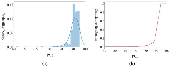
Figure 1.
Overall evaluation of the road network after weighting: (a) Frequency plot; (b) Cumulative distribution plot.
5.3. Road Segment Distribution Sampling Modelling and Clustering
From the analysis in Figure 1, it can be seen that the overall level of the road network is relatively good. It is necessary to further filter out the poor road sections from the road network. The K-means algorithm can be used to cluster the level distribution of road section pavement performance.
First, for each route, a continuous function model of the cumulative distribution of pavement performance indexes is established. Then, set the range of independent variables, and the range and number of independent variables for each route are the same. Here, the value range of the independent variable is set to [0.1, 100], and the number of independent variables is 1000. Therefore, the independent variable domain is [0.1, 0.2,..., 100]. According to the continuous function model, the cumulative distribution of the corresponding index values is calculated, and the cumulative distribution values of each road segment are, respectively, formed into high-dimensional vectors with the same dimensions.
For example, the cumulative distribution vector of pavement properties for R1 is . A road network with n routes contains 15 high-dimensional cumulative distribution vectors, .
The cumulative distribution vector of the pavement performance of the above 15 road sections is used as the observation vector, and K-means clustering is performed to classify the road sections with similar road levels into one category. Set the value of K as an integer value from 1 to 15, calculate the sum of squares of errors after each classification, and draw the relationship between the sum of squares of errors and the value of K in Figure 2. As can be seen from the figure, K = 3 is an ideal value. The initial K value is set to 3, and clustering is performed according to the steps in “Overall evaluation of road network pavement performance”. The clustering results are shown in Table 2 and Figure 3.
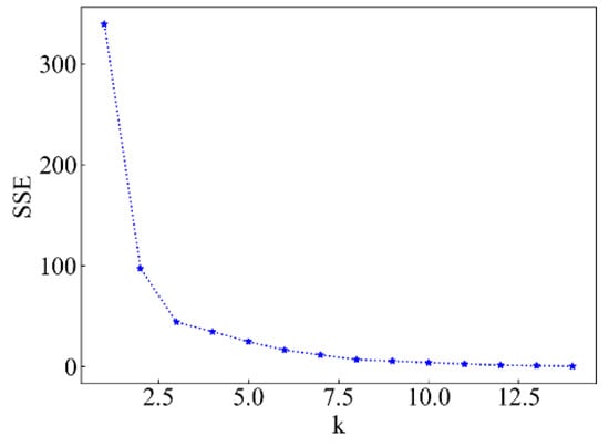
Figure 2.
The relationship between SSE and the number of classes.
Table 2.
Summary of clustering results.
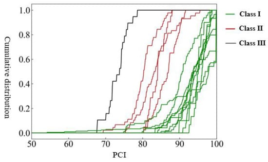
Figure 3.
Clustering diagram obtained by using K-means algorithm based on road performance distribution of road sections (K = 3).
Analyzing Figure 3, the 15 routes are divided into three categories according to the level of pavement performance. Class III includes only one route, R11, and is the class with the worst road performance level.
Class II includes four road sections. The road surface level of these road sections is slightly better than that of R11, but there is no road section with a PCI of 100, and the cumulative distribution reaches one in the 80–90 range.
Class I contains many road sections and belongs to a category with better road performance. However, the composition of pavement performance levels of different road sections is also quite different. In some road sections, the pavement performance level of each road section exists and is balanced from 80 to 100; in some road sections, about 40% of the road sections have a PCI value of 100.
Therefore, K = 3 has already reduced the sum of squared errors to a certain level, and the intra-class similarity is high. However, in practical applications, further clustering is required to further identify road segments with more similar performance decays.
By selecting a number of different K values and observing the clustering results, it is found that K = 5 and K = 8 can better describe the pavement performance decay characteristics of similar routes. The three clustering results are summarized in Table 2, and the pedigree map is drawn in Figure 4. The clustering effects of K = 5 and K = 8 are shown in Figure 5, respectively.
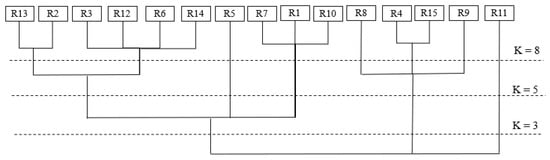
Figure 4.
The clustering pedigree obtained by using the K-means algorithm based on the road segment pavement performance distribution.
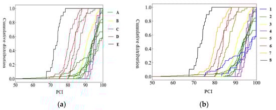
Figure 5.
Clustering diagram obtained using K-means algorithm based on road performance distribution of road sections: (a) K = 5; (b) K = 8.
5.4. Pavement Performance Clustering of Unit Road Sections
After the road segment clustering is completed, further detailed analysis can be carried out on the road segments with low road performance levels or by selecting specific road segments according to project requirements. In this section, R4 is used as an example to cluster unit road segments.
R4 has a total length of 48.32 km and a total of 48 units to evaluate the road sections. Based on its PCI measured data in 2019, a PCI cumulative distribution evaluation model was established through the sampling theorem. The value of the independent variable is set to [0, 100], the sampling point N is set to 1000, and the sampling interval is set to 0.1. The discrete cumulative frequency distribution data of pavement performance indexes are continuous.
The continuation function of the measured value of PCI cumulative distribution and Equation (5) is plotted in Figure 6a. It can be seen from the figure that the PCI cumulative distribution continuity function completely coincides with the field measured value, that is, the modeling fit is very high. By substituting any road performance index level into the function through the continuity equation, the proportion of road sections below the performance index level can be obtained. Similarly, the RQI cumulative distribution evaluation model is established by the sampling theorem, and the fitting result is also high, as shown in Figure 6b below.
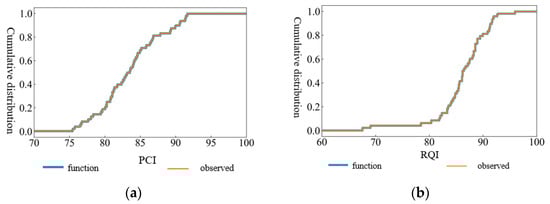
Figure 6.
Continuity graph of the cumulative distribution of R4 pavement performance: (a) PCI; (b) RQI.
The K-means algorithm was used to cluster the R4 unit evaluation road segments. The input observation value is a two-dimensional vector constructed by the R4 unit evaluation road section pavement performance indexes PCI and RQI. There are 48 unit road segment vectors with the station number i.
The calculated K value and its corresponding error sum of squares are shown in Figure 7. It can be seen from the figure that the error sum of squares decreases rapidly from class 1 to class 5, and then decreases slowly, indicating that the ideal K value appears at 5.
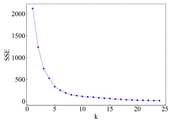
Figure 7.
The relationship between SSE and the number of classes for R4.
Set K = 5, the initial cluster center point is randomly selected from the observation vector, and K-means clustering is performed. The results of the unit evaluation road segment based on PCI and RQI clustering are plotted in Figure 8. The figure takes PCI as the abscissa and RQI as the ordinate. It can be clearly seen that all the observation unit road sections are divided into five categories.
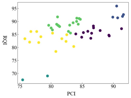
Figure 8.
Five groups of cluster diagrams obtained by using K-means algorithm based on PCI and RQI data.
The cumulative distribution continuation functions for PCI and RQI are plotted in Figure 9. Combining Figure 8 and Figure 9, it can be seen that the PCI index of the two-unit road sections whose RQI index is lower than 70 is also lower than 80, which can be classified into one category, and similar maintenance measures are taken during maintenance. Most of the road sections are in the horizontal range of PCI and RQI of 70–90. According to the clustering results, these road sections can be divided into three categories for research. For the sections with a PCI index higher than 90, the RQI is also higher than 90. These sections with better performance are concentrated in the upper right corner of the cluster map.
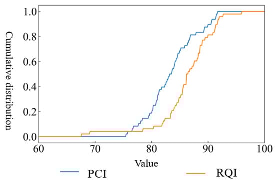
Figure 9.
Continuity function diagram of the cumulative distribution of PCI and RQI.
6. Conclusions
This paper proposes a cumulative distribution modelling method for pavement performance indexes based on the sampling theorem, and implements clustering analysis of similar road sections through the K-means algorithm. The main conclusions are as follows.
(1) The modelling method proposed in this paper can convert discrete pavement performance data into a continuous function of pavement performance indexes and a continuous function of pavement performance cumulative distribution, and achieve the acquisition of a large amount of pavement performance data.
(2) Based on the cumulative distribution and K-means clustering, it is possible to understand the overall pavement performance status of the network and identify road sections with similar decay models and poor decay status for focused attention, which constructed the pavement performance evaluation system of the three-level system of road network–road section–unit road section.
Author Contributions
Conceptualization, Q.Y.; methodology, Q.Y.; software, R.Z.; validation, W.Y., Q.Y. and R.Z.; formal analysis, W.Y.; investigation, W.Y.; resources, W.Y.; data curation, W.Y.; writing—original draft preparation, R.Z.; writing—review and editing, W.Y.; visualization, R.Z.; supervision, Q.Y.; project administration, W.Y.; funding acquisition, W.Y. All authors have read and agreed to the published version of the manuscript.
Funding
This research was funded by 2021 Ningbo Transportation Science and Technology Plan Project, grant number 202119.
Institutional Review Board Statement
Not applicable.
Informed Consent Statement
Not applicable.
Data Availability Statement
Not applicable.
Conflicts of Interest
The authors declare no conflict of interest.
References
- Shrestha, S.; Katicha, S.W.; Flintsch, G.W.; Diefenderfer, B.K. Implementing Traffic Speed Deflection Measurements for Network Level Pavement Management in Virginia. J. Transp. Eng. Part B 2022, 148, 04022021. [Google Scholar] [CrossRef]
- Shtayat, A.; Moridpour, S.; Best, B.; Rumi, S. An Overview of Pavement Degradation Prediction Models. J. Adv. Transp. 2022, 2022, 1–15. [Google Scholar] [CrossRef]
- Sidess, A.; Ravina, A.; Oged, E. A model for predicting the deterioration of the pavement condition index. Int. J. Pavement Eng. 2020, 22, 1625–1636. [Google Scholar] [CrossRef]
- Lin, Z.; Wang, H.; Li, S. Pavement anomaly detection based on transformer and self-supervised learning. Autom. Constr. 2022, 143, 104544. [Google Scholar] [CrossRef]
- Jiang, X.; Gabrielson, J.; Huang, B.; Bai, Y.; Polaczyk, P.; Zhang, M.; Hu, W.; Xiao, R. Evaluation of inverted pavement by structural condition indicators from falling weight deflectometer. Constr. Build. Mater. 2022, 319, 125991. [Google Scholar] [CrossRef]
- Gong, H.; Sun, Y.; Huang, B. Estimating Asphalt Concrete Modulus of Existing Flexible Pavements for Mechanistic-Empirical Rehabilitation Analyses. J. Mater. Civ. Eng. 2019, 31, 04019252. [Google Scholar] [CrossRef]
- Chen, D.; Mastin, N. Sigmoidal Models for Predicting Pavement Performance Conditions. J. Perform. Constr. Facil. 2016, 30, 04015078. [Google Scholar] [CrossRef]
- Haider, S.W.; Baladi, G.Y.; Chatti, K.; Dean, C.M. Effect of Frequency of Pavement Condition Data Collection on Performance Prediction. Transp. Res. Rec. J. Transp. Res. Board 2010, 2153, 67–80. [Google Scholar] [CrossRef]
- Abaza, K.A.; Ashur, S.A. Optimum microscopic pavement management model using constrained integer linear programming. Int. J. Pavement Eng. 2009, 10, 149–160. [Google Scholar] [CrossRef]
- Ouyang, Y.; Madanat, S. Optimal scheduling of rehabilitation activities for multiple pavement facilities: Exact and approximate solutions. Transp. Res. Part A 2004, 38, 347–365. [Google Scholar] [CrossRef]
- Liu, C.; Wu, D.; Li, Y.; Du, Y. Large-scale pavement roughness measurements with vehicle crowdsourced data using semi-supervised learning. Transp. Res. Part C: Emerg. Technol. 2021, 125, 103048. [Google Scholar] [CrossRef]
- Du, E.; Ma, S.; Jing, H. Asphalt Pavement Performance Prediction Model Based on Gray System Theory. J. Tongji Univ. Nat. Sci. 2010, 38, 1161–1164. [Google Scholar]
- Guo, F.; Zhao, X.; Gregory, J.; Kirchain, R. A weighted multi-output neural network model for the prediction of rigid pavement deterioration. Int. J. Pavement Eng. 2021, 23, 2631–2643. [Google Scholar] [CrossRef]
- Kim, S.-H.; Kim, N. Development of performance prediction models in flexible pavement using regression analysis method. KSCE J. Civ. Eng. 2006, 10, 91–96. [Google Scholar] [CrossRef]
- Wang, W.; Wang, S.; Xiao, D.; Qiu, S.; Zhang, J. An Unsupervised Cluster Method for Pavement Grouping Based on Multidimensional Performance Data. J. Transp. Eng. Part B 2018, 144, 04018005. [Google Scholar] [CrossRef]
- Park, S.W.; Suh, Y.C.; Chung, C.G. Development of Prediction Method for Highway Pavement Condition. Int. J. Highw. Eng. 2008, 10, 199–208. [Google Scholar]
- Lijuan, Z.; Jianming, L.; Yunqi, Z.H.U. Gray and Fuzzy Clustering Method-Based on Network Level Pavement Performance Assessment. J. Tongji Univ. Nat. Sci. 2010, 38, 252–256. [Google Scholar]
- Kaya, O.; Ceylan, H.; Kim, S.; Waid, D.; Moore, B.P. Statistics and Artificial Intelligence-Based Pavement Performance and Remaining Service Life Prediction Models for Flexible and Composite Pavement Systems. Transp. Res. Rec. J. Transp. Res. Board 2020, 2674, 448–460. [Google Scholar] [CrossRef]
- Abed, A.; Thom, N.; Neves, L. Probabilistic prediction of asphalt pavement performance. Road Mater. Pavement Des. 2019, 20, S247–S264. [Google Scholar] [CrossRef]
- Kalita, K.; Rajbongshi, P. Variability characterisation of input parameters in pavement performance evaluation. Road Mater. Pavement Des. 2014, 16, 172–185. [Google Scholar] [CrossRef]
- Wojtkiewicz, S.F.; Khazanovich, L.; Gaurav, G.; Velasquez, R. Probabilistic Numerical Simulation of Pavement Performance using MEPDG. Road Mater. Pavement Des. 2010, 11, 291–306. [Google Scholar] [CrossRef]
- Dilip, D.M.; Babu, G.L.S. Influence of Spatial Variability on Pavement Responses Using Latin Hypercube Sampling on Two-Dimensional Random Fields. J. Mater. Civ. Eng. 2014, 26, 04014083. [Google Scholar] [CrossRef]
- Evdorides, H.; Burrow, M.; Sulaiman, S. A methodology to model the variability in pavement performance. Proc. Inst. Civ. Eng. —Transp. 2013, 166, 233–240. [Google Scholar] [CrossRef]
- García-Segura, T.; Montalbán-Domingo, L.; Llopis-Castelló, D.; Lepech, M.D.; Sanz, M.A.; Pellicer, E. Incorporating pavement deterioration uncertainty into pavement management optimization. Int. J. Pavement Eng. 2020, 23, 2062–2073. [Google Scholar] [CrossRef]
- Jia, X.; Huang, B.; Zhu, D.; Dong, Q.; Woods, M. Influence of Measurement Variability of International Roughness Index on Uncertainty of Network-Level Pavement Evaluation. J. Transp. Eng. Part B 2018, 144, 04018007. [Google Scholar] [CrossRef]
- Rose, S.; Mathew, B.S.; Isaac, K.P.; Abhaya, A.S. Risk based probabilistic pavement deterioration prediction models for low volume roads. Int. J. Pavement Eng. 2016, 19, 88–97. [Google Scholar] [CrossRef]
- Luke, H. The origins of the sampling theorem. IEEE Commun. Mag. 1999, 37, 106–108. [Google Scholar] [CrossRef]
- Indebetouw, G.; Lo, K.P.; Ho, K.C. Interpolation theorem for quasi-periodic sampling. JOSA A 1988, 5, 1030–1034. [Google Scholar] [CrossRef]
- Wang, Q.; Wu, L. A sampling theorem associated with quasi-Fourier transform. IEEE Trans. Signal Process. 2000, 48, 895. [Google Scholar] [CrossRef]
- Zhang, W.; Tao, R. Sampling Theorems for Bandpass Signals with Fractional Fourier Transform. Acta Electron. Sin. 2005, 33, 1196–1199. [Google Scholar]
- Agrawal, M.K.; Elmaghraby, S.E. On computing the distribution function of the sum of independent random variables. Comput. Oper. Res. 2001, 28, 473–483. [Google Scholar] [CrossRef]
- Dokmanic, I.; Petrinovic, D. Convolution on the $n$-Sphere With Application to PDF Modeling. IEEE Trans. Signal Process. 2009, 58, 1157–1170. [Google Scholar] [CrossRef]
- Finkelshtein, D.; Tkachov, P. Kesten’s bound for subexponential densities on the real line and its multi-dimensional analogues. Adv. Appl. Probab. 2018, 50, 373–395. [Google Scholar] [CrossRef]
- Katsikadelis, J.T. Numerical solution of integrodifferential equations with convolution integrals. Ingenieur-Archiv. 2019, 89, 2019–2032. [Google Scholar] [CrossRef]
- Maslakov, M.L. New Approach to the Iterative Method for Numerical Solution of a Convolution Type Equation Determined for a Certain Class of Problems. Comput. Math. Math. Phys. 2021, 61, 1260–1268. [Google Scholar] [CrossRef]
- Zhang, G.; Zhu, R. Runge–Kutta convolution quadrature methods with convergence and stability analysis for nonlinear singular fractional integro-differential equations. Commun. Nonlinear Sci. Numer. Simul. 2019, 84, 105132. [Google Scholar] [CrossRef]
- Cipra, T. Financial and Insurance Formulas; Springer Science & Business Media: Berlin/Heidelberg, Germany, 2010. [Google Scholar] [CrossRef]
- McDaniel, L.S.; Glen, A.G.; Leemis, L.M. Linear Approximations of Probability Density Functions. In Computational Probability Applications; Springer: Cham, Switzerland, 2016; pp. 119–132. [Google Scholar] [CrossRef]
- Glen, A.G.; Leemis, L.M.; Drew, J.H. Computing the distribution of the product of two continuous random variables. Comput. Stat. Data Anal. 2004, 44, 451–464. [Google Scholar] [CrossRef]


Disclaimer/Publisher’s Note: The statements, opinions and data contained in all publications are solely those of the individual author(s) and contributor(s) and not of MDPI and/or the editor(s). MDPI and/or the editor(s) disclaim responsibility for any injury to people or property resulting from any ideas, methods, instructions or products referred to in the content. |
© 2022 by the authors. Licensee MDPI, Basel, Switzerland. This article is an open access article distributed under the terms and conditions of the Creative Commons Attribution (CC BY) license (https://creativecommons.org/licenses/by/4.0/).