Non-Destructive Assessment of the Functional Diameter and Hydrodynamic Roughness of Additively Manufactured Channels

Abstract

Metal additive manufacturing, particularly laser powder bed fusion, is increasingly used in the gas turbine industry for the fabrication of channels with small diameters for conformal cooling and flow passage applications. A critical challenge in this context lies in evaluating aspects such as the geometrical and hydraulic diameters, the effective area and the roughness on the internal surface of the channel that affects the flow functionality. This paper proposes a new method to evaluate the geometrical and functional equivalent diameters, i.e., the hydraulic diameter of cylindrical channels and the mean surface topography height on the internal channel surface, using X-ray computed tomography. The developed methods were validated with experimental flow tests, considering the mean surface topography height to be equivalent to the hydrodynamic sand grain roughness, thereby determining the hydraulic diameter and the associated effective area. The method is a much faster approach to determining the available hydraulic diameter compared to flow tests and offers the possibility of evaluating the internal surface characteristics, with discrepancies between the two approaches being less than ±3%.

1. Introduction

Laser powder bed fusion (L-PBF) is one of the fastest-growing metal additive manufacturing technologies because of its capability to fabricate complex geometries with intricate substructures, such as internal channels [1,2,3]. In particular, the fabrication of channels and holes with small diameters has gained continuous interest in advanced manufacturing industries for producing automotive and gas turbine parts. However, the components produced by L-PBF are subjected to high surface roughness. In contrast, the surface irregularities inside of channels strongly depend on the inclination angle, leading to dross formation and stair-case defects on the upward- and downward-facing surfaces [4,5]. These surface irregularities, in the form of microscale features on the internal surface of the channel, can be related to the hydrodynamic sand grain roughness “k_s” or mean roughness height “ε” and were recently introduced as the mean surface topography height (msth) [5]. The hydrodynamic sand grain roughness “k_s” is defined as the mean height of tightly packed protruding sand-grain-like features that are uniformly distributed inside the channel, directly impacting the fluid flow through the channel in terms of the pressure drop due to friction and an alteration from the designed mean channel diameter [6,7,8]. Therefore, the mean channel diameter, affected by the microscale surface irregularities exhibiting msth, needs to be carefully assessed in a non-destructive manner to understand the functionality of the channel [5]. For this purpose, experimental flow tests are generally conducted to determine the hydraulic diameter (d_h), the effective area (A_eff) and, subsequently, the hydrodynamic sand grain roughness (k_s) or mean roughness height (ε) [6,9,10]. In fluid mechanics, the pressure drop due to friction is generally known as the major loss in a pipe, or channel flow, and pressure drops due to geometrical fittings such as elbows, joints, valves, etc., are collectively known as minor losses [11,12]. However, there are constraints related to the experimental setup regarding the channel’s dimensions and geometry under investigation. Hence, different geometries inflict additional complexity in the experimental setup, which can also strongly impact the measurement accuracy. As a result, re-calibration is required whenever modifications are made to the experimental setup, resulting in longer evaluation times and higher costs. Industrial X-ray computed tomography (CT) is a powerful non-destructive technique that enables the assessment and measurement of the component and internal features without altering its actual form and allows a 3D reconstruction of the internal features of a component, such as internal channels [13,14,15]. Several approaches can be applied to the 3D modelling of the CT-scanned part to perform dimensional and geometrical measurements. One approach is the nominal-to-actual comparison of the CT-scanned part (actual) with the computer-aided design (CAD) geometry (nominal).

However, for components with high surface variation, achieving the proper alignment between the actual and nominal geometry becomes increasingly difficult, which in turn can strongly affect the accuracy of the dimensional evaluation [16]. A perfect example of such components is parts manufactured by L-PBF, where high surface variation can originate from several causes. For example, the parts undergo high thermal gradients during production. They are fully immersed in powder at the end of the fabrication process due to the layer-by-layer building process. As a result, the surrounding powder can become attached to the borders of the part due to partial sintering or adhesion forces and can cause deviations from the nominal CAD design file [17]. This effect becomes more prominent in overhanging regions with large inclination angles, which means that the laser beam passes over a section of the powder layer under which only loose powder is present, leading to poorer surface quality due to stair-case effects or sag and dross formations [5,17]. Another similar approach is the fitted-ellipse method applied to the stack of images extracted from the scanned CT volume to determine the internal channel roughness [7]. However, the geometrical shape of the channel imposes a limitation on the length of the section on which the analysis can be performed and therefore hinders the applicability of the method to different geometries.

In this paper, the algorithm for “wall thickness analysis” in VGStudio MAX 3.3 (Volume Graphics GmbH, Germany) is proposed to evaluate the geometrical mean diameter (d_mean), the functional equivalent diameter (d_eq) and the msth of internal channels without the necessity of the alignment between the actual and nominal geometry to avoid dimensional measurement uncertainties, as discussed in [13,14]. These data could be used as essential feedback in the design phase for the evaluation of shape compensation methods to achieve near-net shapes close to the nominal dimensions. In contrast, d_eq, for example, can be correlated with d_h. To validate the proposed methodology, the d_eq values obtained from the wall thickness analysis are compared with the d_h determined with incompressible experimental flow tests performed in the turbulent flow regime. Darcy–Weisbach and Colebrook–White equations are used to evaluate the experimental d_h and A_eff. Section 2 presents the components used in this study and the methodologies involved in performing the CT scan and the wall thickness analysis to determine d_eq and msth. In addition, this section describes the experimental flow test arrangement and the governing equations to determine d_h. Section 3 presents the results obtained from the wall thickness analysis and the experimental flow tests. The results are compared and discussed to validate the proposed methodology, leading to the conclusions, and suggestions for future work are described in Section 4.

2. Materials and Methods

2.1. X-ray Computed Tomography Measurements

The specimens used for the investigation in this study are cylindrical internal channels (N1 and N2) fabricated by L-PBF that were built as a part of an industrial case study from Baker Hughes, Italy. The part was manufactured vertically with an orientation perpendicular to the build platform. The material used for fabrication was INCONEL 718, an austenitic nickel-chromium-based superalloy commonly used for high-temperature applications in gas turbines [3,5]. The channels were cut out from the whole part to obtain separate specimens using Wire Electrical Discharge Machining and individually scanned with CT. The channels consist of an integrated straight and inclined section with an inclination angle of 60° from the horizontal axis and a bend radius of 3 mm. The nominal diameter of channel specimens N1 and N2 are 1.5 mm and 1 mm, respectively. Figure 1 displays the (a) fabricated case study, (b) drafting with the dimensions of the case study and (c) one of the CT-scanned volumes of the individual channel specimen to visualise the 60° bend in the centre of the specimen visualised with respect to the y-axis.

The specimens were scanned using a metrological CT system Nikon MCT 225 (Nikon Metrology X-Tek, Herts, UK), where only the centre part of each specimen was in the field of view to avoid potential defects induced by the cutting and to achieve the highest resolution to resolve and visualise the microscale surface features on the internal surface of the channel. The part was positioned as close as possible to the X-ray source, while it was ensured that the specimen’s complete projection was inside the field of view of the detector at any rotation position. In this way, an 8 mm high section centred around the bend of the channels could be acquired with a voxel size of 4 µm. The optimised scan parameters for the scans are shown in

Table 1. Optimised scan parameters used for CT measurements.

Parameter	Value
Power	6.8 W
Voltage	170 kV
Exposure time	2 s
Number of projections	2000
Filter	0.5 mm tin

and were not altered for the different samples. To reduce beam hardening artefacts due to the high density of the material, a 0.5 mm tin filter was used. The acquired images were reconstructed with the reconstruction software provided by the CT system manufacturer without any additional software filtering or artefact reduction. Subsequently, the volumes were imported in VGStudio MAX 3.3 for further analysis.

After the surface was determined, a Region of Interest (ROI) was created comprising only the internal channel (cf. yellow rectangle in Figure 2) to perform the wall thickness analysis in two different modes (background and material) using the Ray and Sphere methods implemented in VGStudio. Figure 2a shows a schematic representation of the working directions (blue material mode and red arrow background mode) of the different wall thickness analyses on the cross-section of the specimen shown in Figure 1c, while Figure 2b illustrates the creation of individual ROIs for the straight and inclined sections of the channel specimen. Within the ROIs, analyses applying different combinations of both working directions and the Ray and Sphere approaches were conducted, resulting in four data sets that were further processed to determine d_mean and d_eq. Regardless of whether the Ray or Sphere method was used, the background mode operated only on the internal volume of the channels (i.e., non-material voxels) using the determined surface on one side as the starting point to find the closest surfaces within a pre-defined opening angle that was set to 15°. On the other hand, the Sphere method is based on spheres that are incrementally expanded throughout the ROI until the sphere touches two points of the surface.

On the other hand, the material mode determines the thickness distribution of the material between the determined surface and the boundaries of the ROI. To determine the geometrical d_mean, the Ray method in the background mode was used in accordance with [5,18], and the Sphere method was used to determine the functional d_eq and msth. The resulting wall thickness histograms from the different Ray and Sphere methods were exported and processed with an in-house-developed MATLAB script to obtain d_mean, d_h and msth according to [5]. To compare d_mean, d_eq and msth in the straight and inclined sections, the analysis was carried out by creating individual ROIs for the straight and inclined areas of the channel and also considering an ROI for the entire length of the channel.

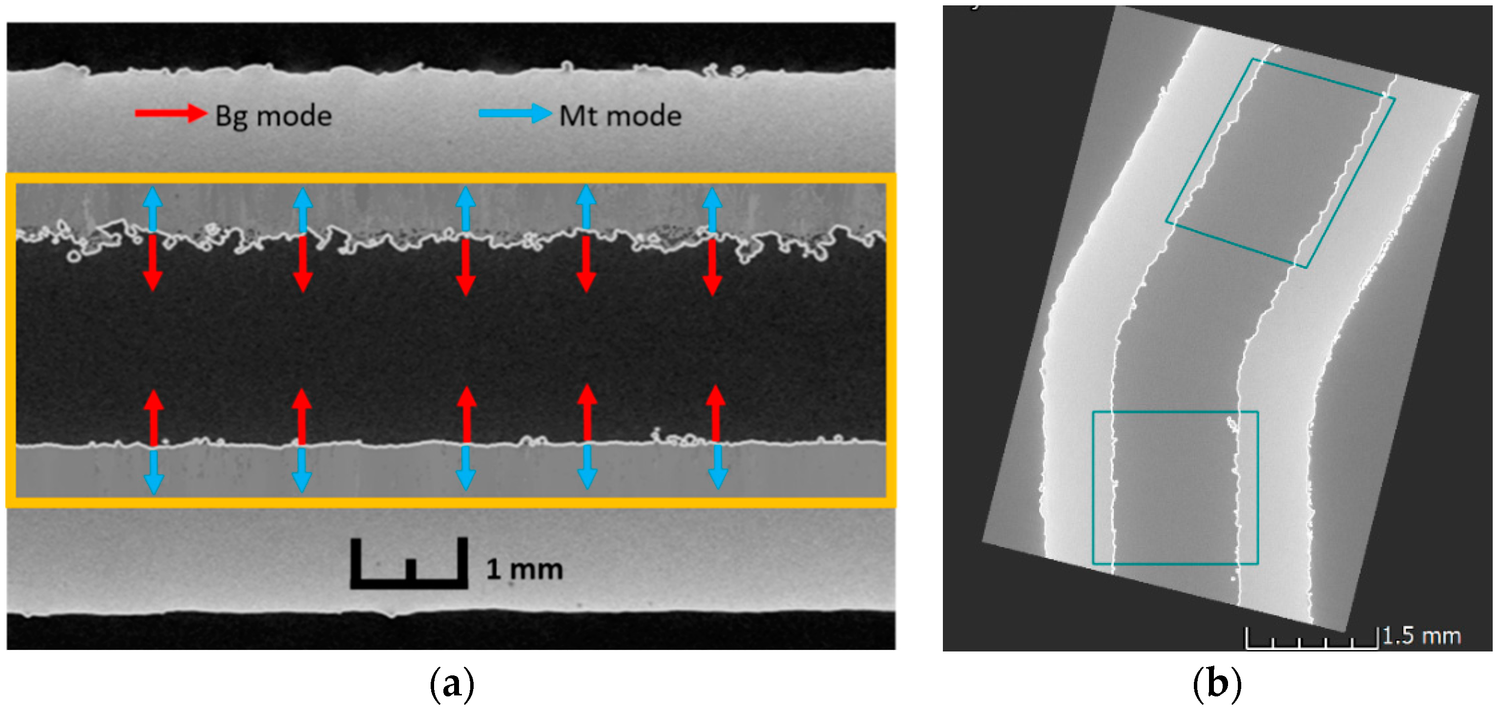
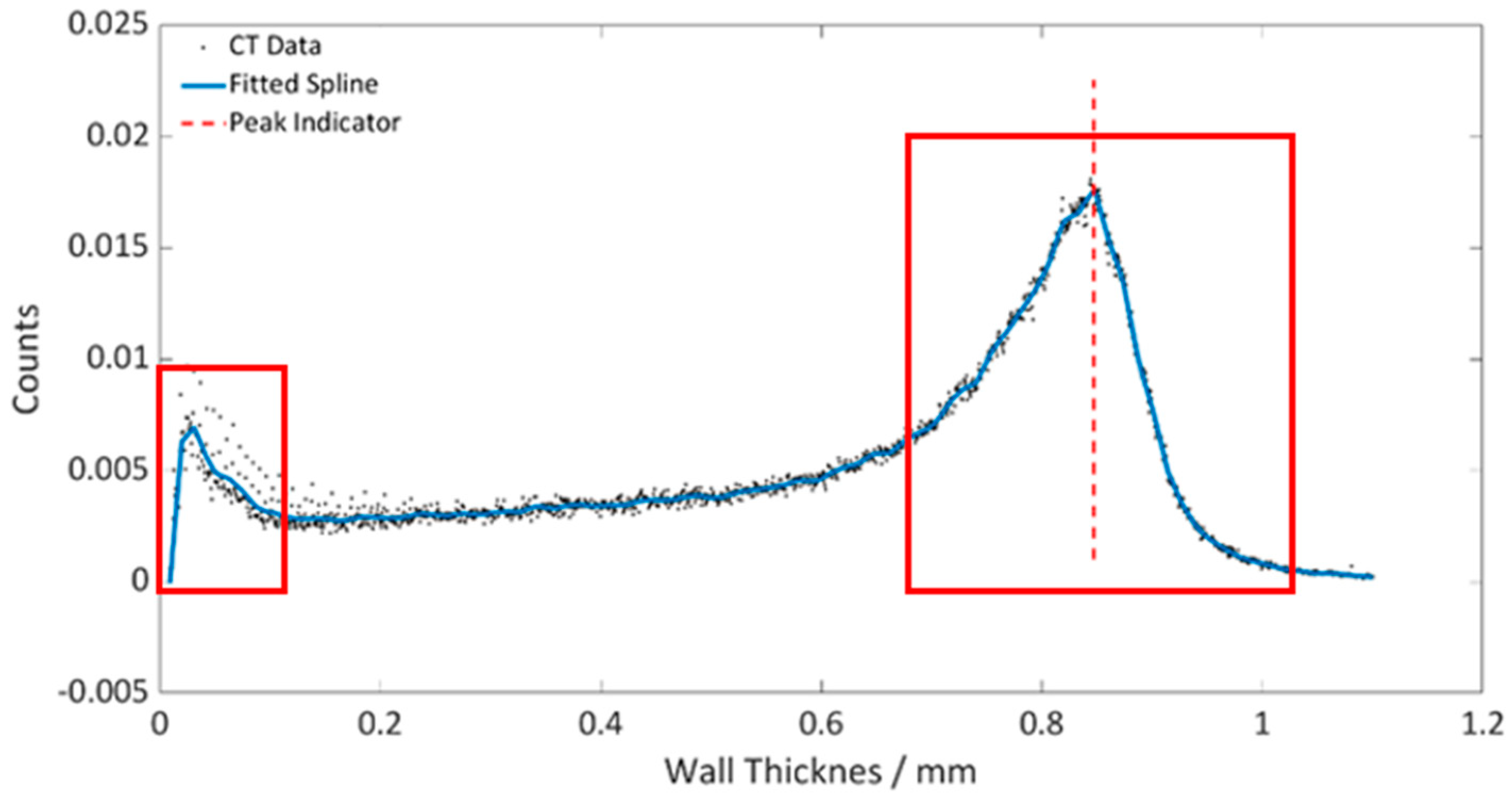
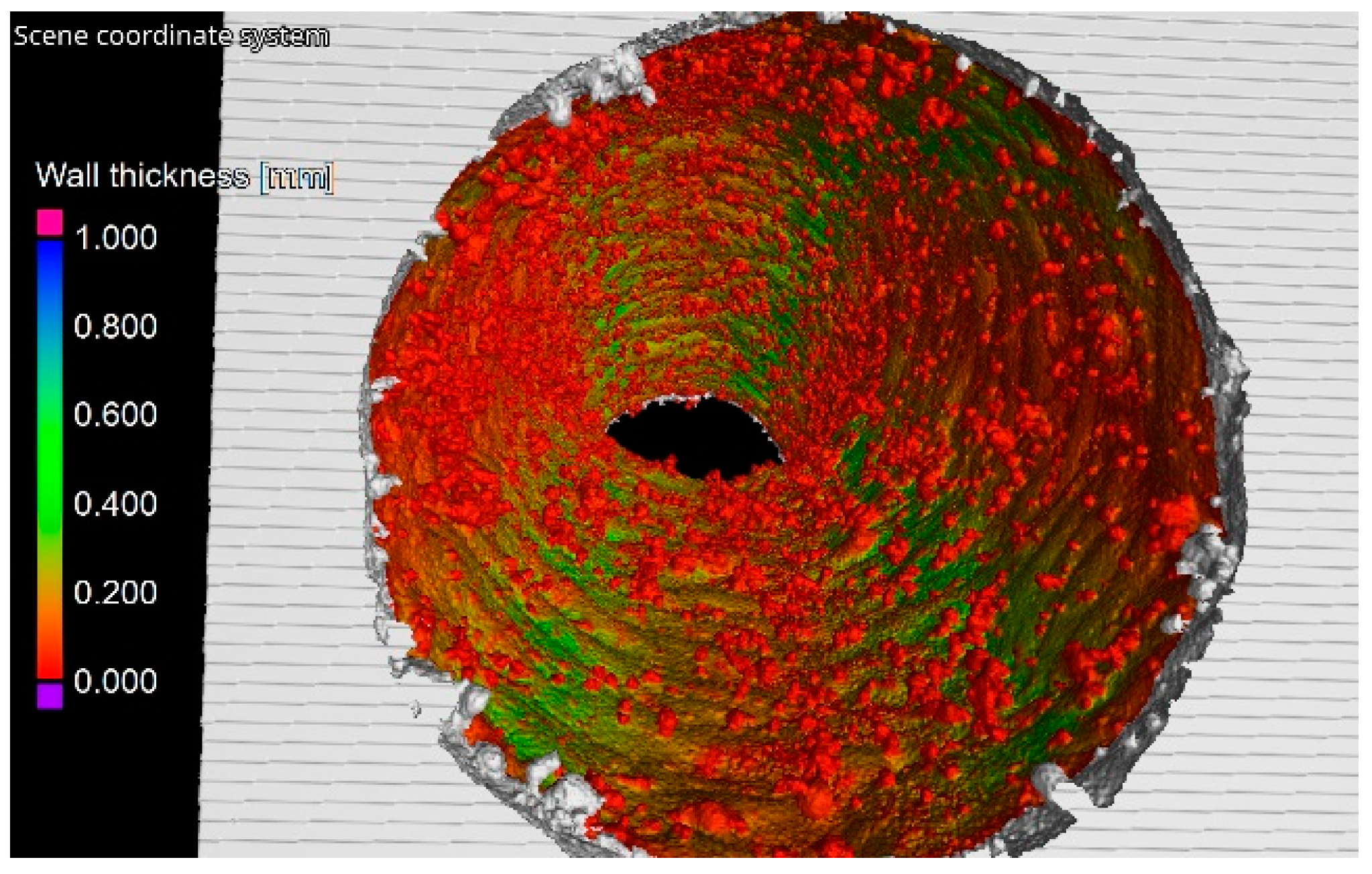
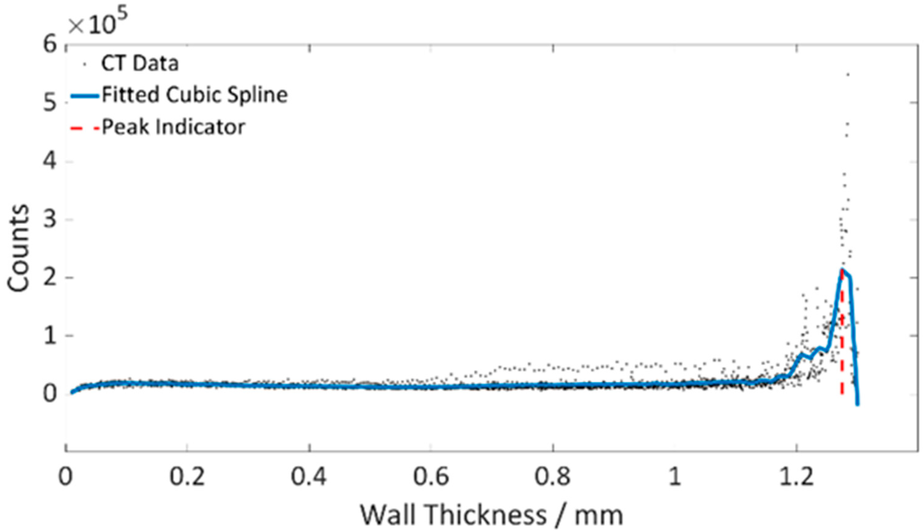
2.2. CT Data Analysis

Prior to the further processing of the extracted histogram data, it is necessary to remove the characteristic periodic spikes in the histograms that are induced due to the finite incremental steps of both wall thickness methods. To achieve this, a search algorithm was implemented to separate the histograms into “standard” data and periodic spikes. After the periodicity of the spikes is determined, a sliding window locally determines the mean value around the spike and resets the value in the particular histogram bin to the determined mean value. To obtain d_mean, d_eq and msth from the adjusted histograms, two different approaches were implemented. The first approach applies a Gaussian fit function to approximate the leading slopes of the peaks corresponding to either the macroscopic channel dimensions, i.e., the diameter, or the msth in microscale features below 200 µm, where the centre position of the Gaussian peak is considered d_mean, d_h or msth. The second approach is based on a search algorithm to determine characteristic peaks in the histograms, whereas the histograms are approximated by applying a non-linear least-squares spline approximation to suppress local variations throughout the different histogram bins. After the peaks were determined in the approximated histogram profile, the corresponding histogram bin positions in the unaltered data were determined to again obtain d_mean, d_eq or msth. To illustrate, Figure 3 shows an example of the adjusted histogram data (black dots) and the corresponding approximation by the non-linear spline. In addition, the two red rectangles indicate the data ranges of small wall-thickness values that were evaluated to obtain msth and of large wall-thickness values that were evaluated to obtain d_mean and d_eq. Within these two ROIs, the values are slightly smoothed with an averaging window function prior to the fit of the Gaussian function.

2.3. Experimental Flow Tests

In order to validate that the diameter values obtained from the Sphere method are equivalent to d_h, experimental incompressible turbulent fluid flow tests were conducted on all of the parts with water as the fluid medium. Figure 4 illustrates a schematic of the experimental setup.

The specimens were flow-tested in the turbulent flow regime while varying the inlet pressure (P₁) upstream of the channel. As a result, for a given inlet pressure, the corresponding mass flow rate ($\stackrel{·}{m}$) was calculated by collecting and measuring the mass of water discharged through the channel per unit of time. The measurements were performed at five different P₁ values on all the specimens. The uncertainty of the entire experimental setup that includes the mass flow and pressure measurements is ±1%. To verify the consistency of the measurements, the flow number was calculated for all five readings. The flow number is a non-dimensional characteristic parameter to evaluate the stability of the fluid flow measurements. The flow measurements are considered consistent and stable when the flow number is found to be constant for all readings. Equation (1) represents the general formulation of the flow number [10].

$$\frac{\stackrel{·}{m}}{{\Delta P}^{\left(0.5\right)}}=Constant$$

(1)

where:

• $\stackrel{·}{m}$—Fluid mass flow rate;
• ΔP—Overall pressure drop.

Concerning the pressure measurements, the pressure at the outlet is considered to be equal to the ambient pressure (P_amb) since water is denser than air. Therefore, the difference between the inlet and outlet pressures is the overall pressure drop (ΔP) or total head loss (H) exerted during the fluid flow through the channel. However, it must be noted that H is the sum of the major and minor losses associated with the flow.

In the case of the experimental setup depicted in Figure 4, the loss at the inlet due to the interconnection with the funnel geometry needs to be considered for both specimens. In addition, the minor loss due to the bend section with an inclination of 30° from the vertical must be regarded for the test parts shown in Figure 1c. The minor losses are calculated by applying a loss coefficient to resolve the general Bernoulli equation. The major loss associated with the flow in all the specimens is the loss due to friction created by the hydrodynamic sand grain roughness (k_s) on the internal surface of the channel [19]. The major loss is calculated using the Darcy-Weisbach and Colebrook-White equation [20]. Equations (2) and (3) represent the Darcy-Weisbach equation in the pressure-loss and head-loss forms, and Equation (4) is the Colebrook–White equation.

$$\frac{{\Delta P}_{friction}}{l}=f_d·\frac{\rho }{2}·\frac{V^2}{d_h}$$

(2)

$$\frac{\Delta h}{l}=f_d·\frac{V^2}{2·g·d_h}$$

(3)

$$\frac{1}{\sqrt{f_d}}=-2log\left[\frac{\epsilon }{3.7·d_h}+\frac{2.51}{R_{ed}\sqrt{f_d}}\right]$$

(4)

where:

• ΔP_friction—Pressure drop due to friction (Pa);
• Δh—Head loss due to friction (m);
• l—Length of the channel (m);
• g—Acceleration due to gravity (m/s²);
• f_d—Darcy–Weisbach friction factor (no unit);
• ρ—Density of the fluid (kg/m³);
• V—Velocity of the fluid flow (m/s);
• d_h—Hydraulic diameter of the channel (m);
• ε—Mean roughness height (m);
• R_ed—Reynold’s number (no unit).

To calculate d_h and the corresponding A_eff, the general Bernoulli energy equation was resolved in terms of overall pressure or head loss from the experiments. The msth obtained from CT is substituted for the mean roughness height (ε) in the Colebrook–White equation [5,19]. Equation (5) represents the re-arranged energy equation, including the summation of minor losses.

$$P_{1-}{P}_2={f_d}^{\ast }·\frac{l·\rho {·V}^2}{d_h·2·g}+\Sigma \xi \frac{V^2}{2·g}$$

(5)

where:

• P₁—Pressure at the inlet of the channel (Pa);
• P₂—Pressure at the outlet of the channel (ambient pressure) (Pa);
• f_d^*—Assumed Darcy–Weisbach friction factor (no unit);
• ξ—Head loss coefficient (no unit);
• V—Velocity of the fluid flow (m/s);
• ρ—Density of the fluid (kg/m³);
• d_h—Hydraulic diameter of the channel (m).

Due to the transition from the funnel-shaped geometry to the inlet of the channel, a minor loss coefficient of 0.8 was applied, and an additional minor loss coefficient of 0.35 was added to consider the losses due to the curvature in the channel geometry [11,12]. To resolve Equation (5), all the velocity parts were converted in terms of d_h to obtain a non-linear equation that can be resolved to determine d_h in an iterative manner by assuming a Darcy–Weisbach friction factor f_d*. Equations (6)–(8) represent the formulation for fluid flow velocity, the non-linear energy equation in terms of d_h and the formulation for Reynold’s number.

$$V=\frac{Q}{A_{eff}}=\frac{4·Q}{{d_h}^2·\pi }$$

(6)

$$\frac{H·g·{\pi }^2}{8·Q^2}·{d_h}^5-\Sigma \xi ·d_h={f_d}^{\ast }·l$$

(7)

$$R_{ed}=\frac{\rho ·V·d_h}{\mu }$$

(8)

Using the Newton–Raphson iterative method, Equation (7) is resolved to obtain d_h based on the convergence criteria when f_d^* = f_d, which is correlated with the aid of the Colebrook–White equation (Equation (4)). This is followed by the determination of Reynold’s number (R_ed) for the particular mass flow rate to verify whether the flow is in the turbulent regime. The entire set of equations is resolved for d_h and A_eff as a mathematical model with an in-house-developed MATLAB code. Finally, the experimental d_h is compared to the diameters obtained from the CT analysis using the Sphere method.

3. Results and Discussion

The results discussed in this paper do not reflect the actual additive manufacturing capabilities of Baker Hughes. They are related to a combination of printing parameters chosen for this specific part and not used for other purposes. Such parameters have yet to be optimised to improve the process capability and are different from the ones used for parts produced at Baker Hughes.

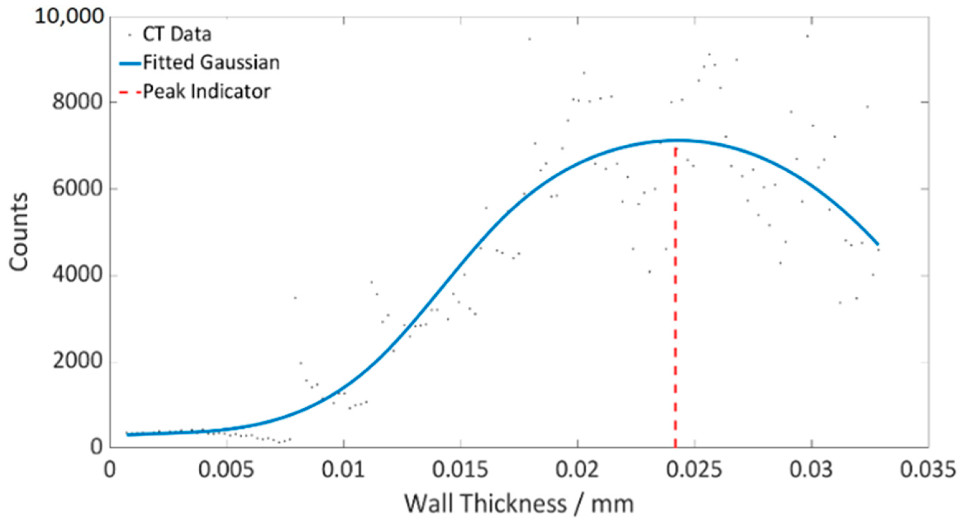
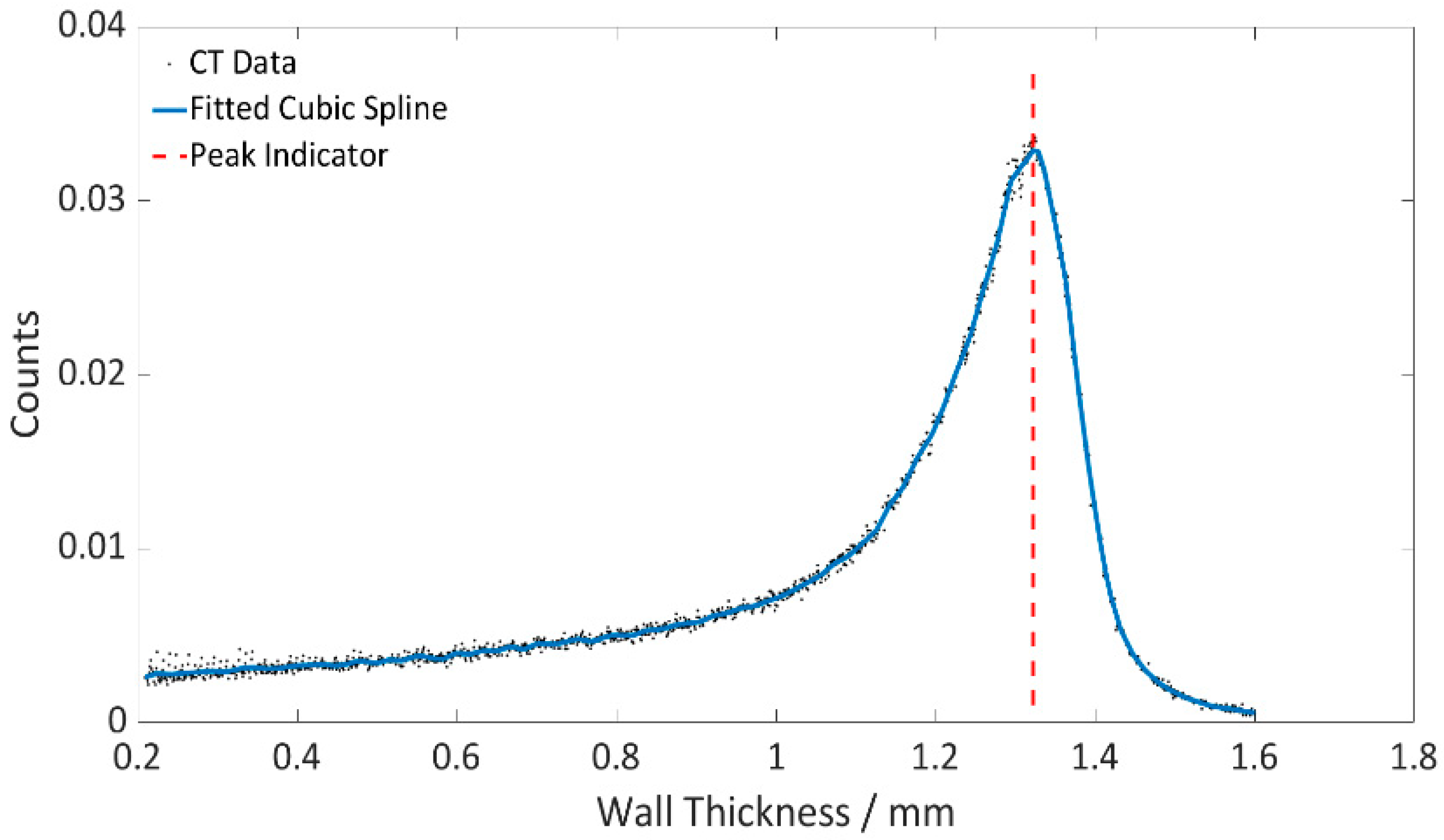
3.1. Wall Thickness Analysis to Determine d_mean, d_eq and msth

In this section, the results obtained from the wall thickness analyses performed on the CT-scanned volumes of specimens N₁ and N₂ are discussed in detail. Figure 5a represents the cross-sectional view of specimen N₁ parallel to the channel direction, analysed in the background mode of the Sphere method within the confined ROI marked in blue, to determine the functional equivalent diameter d_eq, while Figure 5b represents the 3D rendering view of the same. On the other hand, Figure 6 illustrates the 3D rendering view of specimen N₂ as an example of the analysis performed in the material mode of the Sphere method.

It can be seen that the wall thickness analysis using the Sphere method was performed within the confined ROI that is marked in blue in Figure 5a using the background and material modes in both specimens N₁ and N₂ to evaluate d_eq and msth, respectively. When looking at the scale in Figure 6, it becomes evident that the microscale surface features exhibit heights to 100 µm and are distributed in an anisotropic fashion along the length and circumference of the channel.

Figure 7 and Figure 8 show examples of the wall thickness histograms and the corresponding fitted cubic spline curve and Gaussian fits for the wall thickness analysis performed with the Sphere method in background and material modes to determine the equivalent functional diameter d_eq and msth of specimen N₁.

From the peak analysis of the fitted curves, d_eq was found to be 1.27 mm, and the corresponding msth was found to be 24 µm. Furthermore, to determine d_mean, the same procedure was followed for the histograms obtained with the Ray method. Figure 9 represents the wall thickness histogram and the corresponding fitted Gaussian for the wall thickness analysis performed with the Ray method in background mode and a search angle of 15° to determine d_mean. The geometrical mean diameter of the channel was found to be 1.31 mm, which is 190 µm smaller than the design value of 1.5 mm. The data range for the Gaussian fit was chosen around the centre of the main histogram peak considering the histogram data between 1100 µm and 1700 µm. The R-squared value of the fitted Gaussian curve over the CT data was 0.98 in both cases.

The same approach was applied to the histograms of all ROIs of specimens N₁ and N₂ to determine the corresponding d_eq, d_mean and msth, and the results are listed in

Table 2. d_eq, d_mean and msth evaluation for specimens N₁ and N₂.

Part	ROI	dnom/mm	deq/mm (Cubic Spline)	deq/mm (Gaussian Fit)	dmean/mm (Cubic Spline)	dmean/mm (Gaussian Fit)	msth/mm (Cubic Spline)	msth/mm (Gaussian Fit)
N1	F	1.5	1.27	1.27	1.31	1.33	0.024	0.024
N1	S	1.5	1.29	1.29	1.32	1.33	0.024	0.023
N1	I	1.5	1.29	1.29	1.32	1.32	0.024	0.024
N2	F	1	0.79	0.78	0.85	0.84	0.023	0.023
N2	S	1	0.79	0.79	0.85	0.85	0.023	0.022
N2	I	1	0.79	0.78	0.85	0.85	0.023	0.023

. The ROIs for the full-channel section and straight and inclined sections are indicated as F, S and I respectively.

From Table 2, it can be seen that the difference between d_eq and d_mean is consistent in specimens N₁ and N₂ irrespective of the ROI that is analysed. It should also be noted that d_eq and d_mean measured separately at the inclined and straight sections are equivalent to the ones measured along the entire length of the channel, indicating that the deviation from the nominal diameter is constant irrespective of the section of the channel. This kind of analysis of measuring d_mean and d_eq separately at different sections and along the entire length as a single geometry helps in understanding the consistency of the manufacturing process to fabricate channels with bends with different inclination angles. In addition, it can be seen that the measured msth is between 23 µm and 24 µm in both specimens irrespective of the analysed section. This further illustrates that msth is independent of the channel diameter and is more dependent on the material used for fabrication and the L-PBF process parameters. Therefore, msth can be regarded as a surface irregularity parameter that is dependent on the manufacturing process and the material used for fabrication rather than the geometrical dimensions.

3.2. Experimental Flow Test to Determine d_h and A_eff

Generally, experimental flow tests are conducted to determine functional parameters such as the hydraulic diameter (d_h) and the associated effective area (A_eff) of the internal channel to understand their effects on the flow functionality, i.e., the pressure drop at different mass flow rates ($\stackrel{·}{m}$). As discussed in Section 2.3, another important parameter that potentially impacts the flow functionality through the channel is the channel surface irregularity. To investigate the impact, msth determined with the aid of the fitted Gaussian was applied as the hydrodynamic sand grain roughness k_s in the developed mathematical model, and d_h was calculated at different mass flow rates based on the varying inlet pressure.

Table 3. Experimental flow test comparison with CT analysis for the functional hydraulic diameter for specimen N₁.

ΔP (Pa)	H (m)	$\stackrel{\mathbf{·}}{\mathit{m}}$ (kg/s)	Aeff (mm2)	dh (mm) (Flow Test)	deq (mm) (CT)	msth (mm)	fd (No Unit)	V (m/s)	Red (No Unit)	Flow Number (No Unit)
90,500	9.23	0.0084	1.15	1.22	1.27	0.024	0.0547	7.36	8081	0.0088
82,500	8.41	0.0080	1.15	1.22	1.27	0.024	0.0548	7.02	7723	0.0088
69,500	7.09	0.0074	1.15	1.22	1.27	0.024	0.0551	6.45	7129	0.0089
62,000	6.32	0.0071	1.16	1.22	1.27	0.024	0.0553	6.09	6760	0.009
46,500	4.74	0.0062	1.16	1.22	1.27	0.024	0.00559	5.26	5860	0.009

and

Table 4. Experimental flow test comparison with CT analysis for the functional hydraulic diameter for specimen N₂.

ΔP (Pa)	H (m)	$\stackrel{\mathbf{·}}{\mathit{m}}$ (kg/s)	Aeff (mm2)	dh (mm) (Flow Test)	deq (mm) (CT)	msth (mm)	fd (No Unit)	V (m/s)	Red (No Unit)	Flow Number (No Unit)
197,500	20.14	0.0041	0.467	0.77	0.79	0.023	0.064	8.75	6157	0.0029
185,500	18.91	0.0039	0.467	0.77	0.79	0.023	0.064	8.47	5962	0.0029
166,500	16.97	0.0037	0.467	0.77	0.79	0.023	0.0643	8.02	5644	0.0029
153,000	15.60	0.0036	0.467	0.77	0.79	0.023	0.0645	7.69	5422	0.0029
141,500	14.42	0.0035	0.467	0.77	0.79	0.023	0.0646	7.34	5211	0.0029

represent a comparison between d_eq and d_h for specimens N₁ and N₂ determined by experimental flow tests and CT analysis.

From Table 3 and Table 4, it is evident that $\stackrel{·}{m}$ increases with the increase in ΔP. In addition, it can be noted that, for both specimens, the flow number is constant for all ΔP readings, thus confirming the consistency of the experimental setup and the corresponding $\stackrel{·}{m}$ measurements made. Furthermore, the d_h values obtained by resolving the mathematical model described in Section 2.3 are consistent for all $\stackrel{·}{m}$ for specimens N₁ and N_2, irrespective of their different nominal diameters. It can be seen that the Darcy–Weisbach friction factor decreases with the increase in $\stackrel{·}{m}$, indicating the decrease in friction due to the interaction between the fluid and the channel surface with an increase in the fluid flow velocity (V) [11,12,20]. This, in turn, proves the stability of the conducted experiment and also the developed mathematical model.

Upon comparing d_h and the functional equivalent diameter d_eq, a maximum deviation of 50 µm was found in the case of specimen N₁ and 20 µm in the case of specimen N₂. This is observed due to the difference in the deviation between the CT analysis and the experimental flow setup. In addition, the application of msth as an equivalent parameter for k_s is also verified due to the consistency in the determined values of d_h for all $\stackrel{·}{m}$ and the minimum deviation concerning d_eq. Therefore, this comparison helps in understanding the effectiveness of the wall thickness analysis performed in the background mode and material mode of the Sphere method to attain an equivalent parameter to d_h and k_s that could potentially reduce the number of flow tests and thereby reduce the associated evaluation time and cost. Furthermore, this analysis establishes a direct and stable correlation to evaluate the functional characteristics of the component in different fluid flow regimes without the necessity of additional functional models at different $\stackrel{·}{m}$.

4. Conclusions

This study focused on developing a new approach using CT analysis data to determine the functional diameter and internal microscale surface features of cylindrical channels fabricated by L-PBF to link both properties to the flow functionality of the component. The methods developed to analyse the CT data using fitted Gaussian and cubic spline algorithms were compared. They were found to agree in assessing the d_eq, d_mean and msth of internal channels with or without inclination angles.

The functional equivalent diameter obtained from the CT data was further verified by a comparison with the calculated hydraulic diameter (d_h) from experimental flow tests, showing deviations of less than 4% and 2.5% for specimens N₁ and N_2, respectively. The CT data analysis also verified that msth could be introduced as a surface irregularity parameter for channels and is dependent on the manufacturing process and the material used for fabrication rather than the geometrical dimensions.

The method of substituting msth for hydrodynamic sand grain roughness (k_s) in circular channels to determine the experimental d_h was verified with the aid of the developed mathematical model and was proven to be consistent at all mass flow rates in the turbulent flow regime for incompressible flow, thereby avoiding the necessity to develop fluid flow functional models at different $\stackrel{·}{m}$.

The results presented in this work are the first proof of concept to correlate the geometrical characterisation to its functional characteristics based on incompressible fluid flow experiments. Future work will include the CT analysis of an entire component with internal channels and study the effect of internal channel surface irregularities by considering the compressibility effects.

References

1. Brandt, M. Laser Additive Manufacturing Materials, Design, Technologies and Applications; Woodhead Publishing Series in Electronic and Optical Materials: Number 88; Woodhead Publishing: Sawston, UK, 2016. [Google Scholar]
2. Han, P. Additive Design and Manufacturing of Jet Engine Parts. Eng. J. 2017, 3, 648–652. [Google Scholar] [CrossRef]
3. Chandrabalan, L.; Matoni, E.; Malarco, M.; Del Puglia, E.; Ammannato, L.; Carmignato, S. Investigation on precision of laser powder bed fusion process using statistical process control. In Proceedings of the Joint Special Interest Group Meeting between euspen and ASPE Advancing Precision in Additive Manufacturing, Nantes, France, 16–18 September 2019. [Google Scholar]
4. Charles, A.; Elkaseer, A.; Thijs, L.; Hagenmeyer, V.; Scholz, S. Effect of Process Parameters on the Generated Surface Roughness of Down-Facing Surfaces in Selective Laser Melting. J. Appl. Sci. 2019, 9, 1256. [Google Scholar] [CrossRef]
5. Chandrabalan, L.; Baier, M.; Meloni, R.; Ammannato, L.; Del Puglia, E.; Carmignato, S. Assessment and verification of mean effective diameter of internal channels fabricated by laser powder bed fusion. Procedia CIRP 2020, 94, 414–418. [Google Scholar] [CrossRef]
6. Stimpson, C.K.; Snyder, J.C.; Thole, K.A.; Mongillo, D. Scaling roughness effects on pressure loss and heat transfer of additively manufactured channels. J. Turbomach. 2017, 139, 021003. [Google Scholar] [CrossRef]
7. Klingaa, C.G.; Zanini, F.; Mohanty, S.; Carmignato, S.; Hattel, J.H. Characterization of Geometry and Surface Texture of AlSi10Mg Laser Powder Bed Fusion Channels Using X-ray Computed Tomography. Appl. Sci. 2021, 11, 4304. [Google Scholar] [CrossRef]
8. Arshad, F.F.; Rieke, H.H. Surface-Roughness Design Values for Modern Pipes. SPE Drill. Complet. 2006, 21, 212–215. [Google Scholar] [CrossRef]
9. Stimpson, C.K.; Snyder, J.C.; Thole, K.A.; Mongillo, D. Roughness Effects on Flow and Heat Transfer for Additively Manufactured Channels. J. Turbomach. 2016, 138, 051008. [Google Scholar] [CrossRef]
10. Williams, A. Combustion of Liquid Fuel Sprays; Butterworth-Heinemann: Oxford, UK, 1990. [Google Scholar]
11. Idel’chik, I.E.; Fried, E. Flow Resistance A Guide for Engineers, 1st ed.; CRC Press: Boca Raton, FL, USA, 1989. [Google Scholar]
12. Idel’chik, I.E. Memento des Pertes de Charge: Coefficients de Pertes de Charges Singulieres et de Perte de Charges par Frottement, 3rd ed.; Eyrolles: Paris, France, 1986. [Google Scholar]
13. Kraemer, A.; Lanza, G. Assessment of the measurement procedure for dimensional metrology with X-ray computed tomography. In Proceedings of the 14th CIRP Conference on Computer Aided Tolerancing (CAT), Gothenburg, Sweden, 18–20 May 2016; pp. 362–367. [Google Scholar]
14. Aloisi, V.; Carmignato, S. Influence of surface roughness on X-ray computed tomography dimensional measurements of additive manufactured parts. Case Stud. Nondestruct. Test. Eval. 2016, 6, 104–110. [Google Scholar] [CrossRef]
15. Carmignato, S.; Dewulf, W.; Leach, R. Industrial X-ray Computed Tomography; Springer International Publishing: Berlin/Heidelberg, Germany, 2018; ISBN 978-3-319-59571-9. [Google Scholar]
16. Kruth, J.P.; Bartscher, M.; Carmignato, S.; Schmitt, R.; de Chiffre, L.; Weckenmenn, A. Computed Tomography for Dimensional Metrology. CIRP Ann. Manuf. Technol. 2011, 60, 821–842. [Google Scholar] [CrossRef]
17. Baier, M.; Sinico, M.; Witvrouw, A.; Dewulf, W.; Carmignato, S. A novel tomographic characterisation approach for sag and dross defects in metal additively manufactured channels. Addit. Manuf. 2021, 39, 101892. [Google Scholar] [CrossRef]
18. Zanini, F.; Sbettega, E.; Sorgato, M.; Carmignato, S. New Approach for Verifying the Accuracy of X-ray Computed Tomography Measurements of Surface Topographies in Additively Manufactured Metal Parts. J. Nondestruct. Eval. 2019, 38, 12. [Google Scholar] [CrossRef]
19. Kilpatrick, E.; Sung, K. Roughness effects on flow and heat transfer in a ribbed duct considering additive manufacturing. In Proceedings of the Global Power and Propulsion Society Forum, Zurich, Switzerland, 10–12 January 2018. [Google Scholar]
20. Nikuradse, J. Stromungsgesetz in rauhren rohren, vDI Forschungshefte 361. English translation: Laws of flow in rough pipes. In Technical Report, NACA Technical Memorandum, 1292; National Advisory Commission for Aeronautics (NASA): Washington, DC, USA, 1933. [Google Scholar]
Figure 1. Industrial case study with nominal channel diameters of 1.5 mm and 1 mm: (a) picture of the geometry produced by L-PBF; (b) drafting with dimensions of the case study; (c) cut section of CT-scanned case study volume to visualise the 60° bend, with the blue box indicating the created Region of Interest.
Applsci 13 05911 g001
Figure 2. Cross-section of specimen N1 (a) with the ROI denoted in yellow. The red and blue arrows represent the analysis direction for background and material modes of the wall thickness analysis. (b) Individual ROIs indicated in blue for straight and inclined sections of specimen N1.
Applsci 13 05911 g002
Figure 3. Example of adjusted histogram data and corresponding approximation by B-spline, with red rectangles on the left and right indicating the data ranges of small wall-thickness values that were evaluated to obtain msth and of large wall−thickness values that were evaluated to obtain dmean and deq.
Applsci 13 05911 g003
Figure 4. Schematic representation of the experimental flow test setup indicating the direction of the flow and the corresponding pressure measurements.
Applsci 13 05911 g004
Figure 5. CT scanned volume of specimen N1. (a) Cross−sectional view of specimen N1 parallel to the channel direction, analysed in the background mode of the Sphere method within the confined ROI; (b) 3D rendering view of specimen N1 analysed in the background mode of the Sphere method.
Applsci 13 05911 g005
Figure 6. The 3D rendering view of specimen N1 analysed in the material mode of the Sphere method, revealing the microscale surface features in red.
Applsci 13 05911 g006
Figure 7. Wall thickness histogram with fitted cubic spline for functional equivalent diameter (deq) for specimen N1.
Applsci 13 05911 g007
Figure 8. Wall thickness histogram with fitted Gaussian for msth for specimen N1.
Applsci 13 05911 g008
Figure 9. Wall thickness histogram with fitted Gaussian for geometrical mean diameter (dmean) for specimen N1.
Applsci 13 05911 g009