Abstract
In engineering practice, properly characterizing the spatial distribution of soil liquefaction potential and induced surface settlement is essential for seismic hazard assessment and mitigation. However, geotechnical site investigations (e.g., cone penetration test (CPT)) usually provide limited and sparse data with high accuracy. Geophysical surveys provide abundant two-dimensional (2D) data, yet their accuracy is lower than that of geotechnical investigations. Moreover, correlating geotechnical and geophysical data can effectively reduce site investigation costs. This study proposes a data-driven adaptive fusion sampling strategy that automatically develops an assessment model of the spatial distribution of soil liquefaction potential from spatially sparse geotechnical data, performs monitoring of liquefaction-induced settlement, and integrates spatiotemporally unconstrained geophysical data to update the model systematically and quantitatively. The proposed strategy is illustrated using real data, and the results indicate that the proposed strategy overcomes the difficulty of generating high-resolution spatial distributions of liquefaction potential from sparse geotechnical data, enables more accurate judgment of settlement variations in local areas, and is an effective tool for site liquefaction hazard analysis.
1. Introduction
Soil liquefaction is an important research field in geotechnical earthquake engineering, and liquefaction-induced surface settlement is one of the main causes of infrastructure damage during earthquakes [1,2]. Therefore, a reasonable assessment of the spatial distribution of soil liquefaction potential and liquefaction-induced surface settlement can effectively prevent significant casualties and economic losses due to damage [1]. The simplified liquefaction trigger procedure proposed by Seed and Idriss [3] to assess the site liquefaction potential based on a cone penetration test (CPT) is widely accepted internationally. It is well known that the spatial variability of soil properties has a significant impact on soil liquefaction, yet the traditional simplified procedure only provides liquefaction analysis of one-dimensional (1D) spatial soils [4,5]. In addition, this procedure combines the potential volumetric strain of the soil with depth for settlement measurements, which may produce an unreliable liquefaction risk assessment with many limitations [6].
Nowadays, Bayesian methods have been widely applied in geotechnical engineering, such as the characterization of model uncertainties [7,8,9,10], updating of geotechnical parameters [1,11], and seismic liquefaction assessment and monitoring of liquefaction-induced settlement [12,13]. Bayesian compressive sensing/sampling (BCS) is an application of Bayesian methods in compressive sensing or sampling (CS) for efficient reconstruction of signals or images at low sampling rates [14]. It has been used in 1D, 2D, and 3D scenes to reconstruct data points in high-resolution space from sparse CPT soundings and can be effectively applied in geotechnical site investigations [15,16].
In recent years, evaluating the spatial distribution of soil liquefaction potential combined with advanced computer techniques for seismic hazard analysis and mitigation has been developing and is a current research hotspot [17]. For example, Chen et al. performed a probabilistic and spatial assessment of liquefaction-induced settlement by a multiscale random field model [2]. Guan and Wang used Bayesian compressive sampling (BCS) and Monte Carlo to simulate soil spatial variability, as well as to assess liquefaction-induced ground inhomogeneous settlement and lateral displacement [15,16,18]. In addition, CPT-sounding data are often sparsely acquired at specific sites due to time, cost, and access to the subsurface space. The combination of 2D soil stratigraphy and engineering property modeling methods allows smart sampling strategies that characterize the spatial distribution of soil liquefaction potential to quantify interpolation uncertainty and spatial variability [17].
Existing smart sampling strategies include the use of information entropy combined with BCS by Zhao et al. [19] and Zheng et al. [20] to characterize the spatial variability of soil properties and the spatial distribution of liquefaction potential which require consideration of additional CPT soundings and a large budget. It is worth noting that CPT soundings provide highly accurate and directly measured intrusive data, but sparse data make it difficult to develop reliable geostatistical models for cross-sections [21]. Geophysical data are usually acquired independent of site conditions (e.g., multichannel analysis of surface waves (MASW)), but indirectly acquired non-intrusive data contain large uncertainties. Geotechnical and geophysical data are usually correlated, and it is beneficial to integrate geotechnical and geophysical data during site characterization [22,23]. In addition, existing investigations require the fusion of data during site characterization using site-specific empirical equations for geotechnical and geophysical data. For example, Adewoyin et al. [23] used empirical equations to estimate geotechnical parameters, such as Young’s modulus, density, and bulk modulus from seismic wave velocities. Huang et al. [22] proposed a Bayesian framework for integrating CPT and MASW data for the probabilistic characterization of 2D soil profiles. The above methods require consideration of site-specific empirical equations. Therefore, Xu et al. [24] proposed a multi-source Bayesian compressive sampling method for 2D data fusion, fusing geotechnical and geophysical data for 2D subsurface site characterization.
Based on the above theory, this study proposes a data-driven adaptive fusion sampling strategy that automatically develops an assessment model of the spatial distribution of soil liquefaction potential from spatially sparse geotechnical data, performs monitoring of liquefaction-induced settlement, and integrates spatiotemporally unconstrained geophysical data to update the model systematically and quantitatively. It contains three major components, site modeling using sparse geotechnical data from CPT soundings via 2D Bayesian compressive sampling (2D BCS), consolidation settlement modeling combining domain knowledge with CPT-based liquefaction procedures, and multi-source fusion Bayesian compressive sampling (MSF-BCS) coupled with information entropy to automatically fuse sampling samples of geotechnical and geophysical data in a self-adaptive and determine the optimal sampling locations. The reliability level of the spatial assessment target of liquefaction potential is finally achieved, and the interpolation uncertainty and soil spatial variability are quantified. The remainder of this study is organized as follows. Firstly, the simplified CPT-based procedure and site settlement model, as well as the 2D BCS theory, are presented. In addition, the proposed MSF-BCS is presented in detail. Finally, real data are used to illustrate and validate the proposed sampling strategy.
2. Framework of Adaptive Fusion Sampling Strategy
This study proposes an adaptive fusion sampling strategy, which is detailed in the following steps, and a simplified framework is shown in Figure 1.
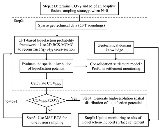
Figure 1.
Framework of adaptive fusion sampling strategy.
In Step 1, the target reliability level () for the spatial distribution assessment of liquefaction potential is determined as the threshold for the adaptive fusion sampling strategy process and the initial number of CPT soundings () is determined, in this case, the number of fusion samples . In Step 2, the CPT-based liquefaction probability assessment framework is used to determine the sampling spacing for preliminary CPT sounding from prior knowledge in the geotechnical domain, and the corresponding sparse data points are derived using the measured cone penetration resistance () and sleeve friction () (sparse data along the horizontal direction). The cross-section is then reconstructed from the sparse data using 2D BCS and Markov chain Monte Carlo (MCMC) simulation to evaluate the spatial distribution of soil liquefaction potential using a version of liquefaction probability developed by Ku et al. [25]. Liquefaction-induced settlement monitoring is performed in conjunction with consolidation settlement theory in the geotechnical domain.
In Step 3, for the sampling strategy to automatically fuse the sampled samples of geotechnical and geophysical data in a self-adaptive manner and determine their optimal sampling locations, a reliability level that can explain ( represents sample data) is defined in the process of Steps 1–3. When the obtained reliability level does not achieve the target reliability level (), MSF-BCS is used to perform a fusion sampling to trigger the adaptive process, which is combined with the information entropy theory to determine the optimal locations for fusion sampling to finally achieve the target reliability level ().
Uncertainty in the sparse data simulated cross-section is quantified using information entropy. represents the information entropy of the cross-section obtained by 2D BCS using geotechnical data from previous CPT soundings, and represents the new information entropy of the cross-section obtained by fusion sampling provided by MSF-BCS. The optimal location for fusion sampling is determined to be the location that maximizes between and . It is worth noting that the maximization has been computed in the process of Steps 1–3.
In Step 4, a high-resolution cross-section is generated from the data points obtained in Step 3 that reach the target reliability level. The high-resolution spatial distribution of liquefaction potential is subsequently generated based on the liquefaction probability assessment framework of CPT. In Step 5, liquefaction-induced surface settlement is updated to quantitatively evaluate the potential for building damage for geotechnical design.
3. CPT-Based Simplified Liquefaction Procedure and Consolidation Settlement Model
3.1. CPT-Based Liquefaction Probability Assessment Framework
A CPT-based liquefaction probability framework was proposed by Robertson and Wride [26] and subsequently updated by Robertson [27]. The ratio of soil liquefaction resistance (expressed as the cyclic resistance ratio ()) to seismic demand (expressed as the cyclic stress ratio ()) was quantified using the factor of safety () for soil liquefaction:
When , liquefaction occurs at the assessment site for a given seismic scenario, provides the soil resistance, which is a function of the equivalent cone penetration resistance in clean sand () and can be expressed as:
where is a function of soil particle properties. is a correction factor, which can be expressed as a soil behavior type index ().
where ,, and . is the total vertical stress, is the normalized cone penetration resistance , , and is the effective vertical stress and the index .
Combined with that suggested by Youd et al. [28], the simplified equation for is as follows:
where represents the peak horizontal acceleration at the surface, represents the acceleration of gravity, and represents the overburden correction factor, assuming a determination factor of , and the quantified equation for the magnitude scaling factor as .
The stress reduction coefficient () is a function of depth :
The simplified procedure for is subject to significant uncertainty, but the calculated is used as a reference for developing the through site case calibration, attenuating this uncertainty [29]. Therefore, to obtain a reliable spatial distribution of liquefaction potential over the whole cross-section, 2D BCS is used to model the within the cross-section from sparse CPT measurement data and to estimate the spatial distribution of liquefaction potential. Ku et al. [25] developed a probabilistic version of Robertson and Wride’s method, denoted as:
where represents the probability of liquefaction and represents the standard normal cumulative distribution function. It is worth noting that to achieve the above mapping function relationship, must follow the calculation of Equations (1)–(5).
3.2. Assessment of Liquefaction-Induced Site Settlement
Soil liquefaction-induced settlement can cause significant damage to buildings on the ground surface, and therefore characterizing soil spatial variability in engineering practice plays an important role in seismic hazard assessment and mitigation. Assuming that the site is in level ground conditions, the liquefaction-induced surface reconsolidation settlement is estimated at the depth of interest () based on a one-dimensional model that estimates liquefaction-induced surface settlement () by integrating the volume strain () [12,30].
where represents the maximum of interest z. The formed during soil reconsolidation is related to the maximum cyclic shear strain () and the relative density of soil () [31]. Therefore, can be expressed as a function of and .
Idriss and Boulanger [32] studied soil liquefaction during earthquakes and proposed a relationship between and and limiting shear strain constraints ():
where the boundary parameters () and can be expressed using as:
The spatial variation of surface reconsolidation was estimated by Equations (1)–(11). Although there are many uncertainties and approximations in the model for estimating , the results estimated using the proposed method provide valuable insights for evaluating the spatial distribution of surface settlement [18]. This study extends the 1D settlement model combined with 2D BCS to 2D space. It is worth noting that the settlement model used only estimates the settlement associated with soil liquefaction followed by reconsolidation, without considering the effects of soil-structure interactions and settlement due to ejecta [12].
4. 2D Bayesian Compressive Sampling (2D BCS)
Bayesian compressive sensing/sampling (BCS) is an application of Bayesian methods in compressive sensing/sampling (CS) to efficiently reconstruct signals or images at low sampling rates. Recently, 2D BCS for reconstructing high-resolution cross-sections of data points from sparse CPT soundings has gained considerable attention and is increasingly used in geotechnical field investigations [15,16,17]. Mathematically, the reconstruction of geotechnical data cross-sections with high resolution from sparse measurement data can be represented by an data matrix . An matrix
and an matrix represent the data points estimated directly from CPT soundings on and the geotechnical data cross-sections reconstructed from , respectively [18]. Theoretically, is represented by a weighted sum of 2D basis functions [33,34].
where and are the -th () 2D basis function and the corresponding weight coefficients, respectively. Let matrix and matrix represent two one-dimensional orthogonal matrices, obtained by the discrete cosine transform (DCT). can be conveniently constructed by and [35]. It is a worthwhile note that for the spatially autocorrelated data points, the values are close to zero except for a few with non-trivial weight coefficients , thus providing the theoretical feasibility of reconstructing geotechnical data cross-sections using sparse measurement data [36]. Mathematically, the CPT measurement data can be constructed using the submatrix of the 2D basis function [20].
where is the measurement matrix specific to this study, reflecting the locations of the CPT soundings along the horizontal direction. The superscript indicates the transpose operation of the matrix.
5. Multi-Source Fusion Bayesian Compressed Sampling (MSF-BCS)
5.1. Multi-Source Bayesian Compressive Sampling (MS-BCS)
In engineering practice, geotechnical investigations provide highly accurate and directly measured intrusive data, however, the data obtained are limited and sparse due to time, cost, and access to the subsurface space. Geophysical data are usually acquired independent of site conditions (e.g., MASW), but indirect, non-intrusive data are obtained [22,37,38].
Xu et al. [24] proposed a novel method of multi-source Bayesian compressive sampling to fuse geotechnical and geophysical data for two-dimensional subsurface spatial variability characterization, which fully exploits the advantages of both data. It is worth noting that this method is not limited by soil type, does not require empirical equations between geotechnical and geophysical data, and prior information in the geotechnical domain, and has significant advantages. Xu et al. [24] used maximum likelihood estimation in obtaining the posterior distribution, which may be more effective for simple models and small data sets. However, this method cannot consider the parameter uncertainty and prior information, which may lead to problems, such as over-fitting and under-fitting. Moreover, considering that most current geotechnical engineering models are highly nonlinear, it is difficult to perform integral solutions in high-dimensional parameter spaces [39].
For complex models and large data sets in geotechnical engineering, this study uses Markov Chain Monte Carlo (MCMC) simulation to integrate prior information in the posterior distribution, which can lead to more accurate and comprehensive estimation results. It is further extended to the study of 2D soil liquefaction potential assessment by adaptively performing multi-source fusion sampling with a reduced amount of field measurement works, and this smart sampling strategy will perform the fusion of geotechnical investigation data (CPT measurement data) and geophysical data (MASW), as described in detail below.
In the BCS framework, most of the non-trivial 2D basis functions in the two highly correlated datasets are similar, and most of the non-trivial 2D basis functions with relatively large weight values can be common for these two correlated CPT measurement data and MASW data. Therefore, the common hyperparameter can be used for and [40]. The cone penetration resistance () is used as the primary variable and the shear wave velocity () data obtained by MASW are used as auxiliary variables to improve the sparse data of the primary variable by data fusion. Cross-sections are represented by the matrix , and in the following the superscripts and represent geotechnical data () and geophysical data (), respectively. Zhao et al. [33,35] identified and estimated from the sparse measured data in Bayesian framework, allowing to be properly reconstructed () with the approximation
where is the likelihood function, reflecting the plausibility of observing given ; is the prior probability density function (PDF) of , reflecting the prior knowledge in the absence of ; is a normalizing constant that ensures that the integration of the posterior distribution is unity. According to the analytical posterior PDF description of conditioned on variables , , and by Zhao et al. [35], the posterior PDF follows a multivariate Gaussian distribution, which can be expressed as
the mean and covariance matrices of are:
where , , represents the Kronecker product in linear algebra. is an matrix with diagonal elements (), follow a Gamma distribution:
where , . Moreover, , . It is worth noting that also follows the Gamma distribution, , where (let ) and (let ). follows a generalized inverse Gaussian distribution, which is represented as [34]:
where , , . In addition, Kp(·) is a modified Bessel function of the second type with parameter . The distribution of is based on αm and and is a multivariate Gaussian distribution. With these conditional probability density functions (PDFs) mentioned above, the posterior PDF of can be obtained by MCMC and detailed procedure is referred to Zhao et al. [35]. In this process, the posterior PDF of
is calculated by determining the common hyperparameter and the union of the non-trivial 2D basis functions. Finally, the estimated and the chosen union can be used to obtain the geotechnical data based on Equation (19). For 2D cross-sectional measurement data are statistically sampled, and the mean () and covariance matrix () of each sampled element are expressed as:
where is a vector of length corresponding to rearranged in increasing order of (). Equation (19) shows that given 2D cross-sectional measurement data , in particular those at unsampled positions of , can be sampled according to the sampling standard deviation given by and , while for each measurement in the 2D cross-section is a weighted sum of [41]. A high-resolution cross-section is then generated from the data (using to represent the sample data) based on CPT’s liquefaction probability assessment framework.
5.2. Determination of the Optimal Location for Fusion Sampling
The concept of information entropy was first introduced in information theory by Shannon [41] to quantify the uncertainty of random processes. A random process with large information entropy is considered to have high uncertainty. The procedures in Section 4 and Section 5.1. are combined with information entropy to determine the optimal location for MS-BCS to perform sampling. The uncertainty of the sparse data simulation cross section can be quantified using information entropy.
represents the information entropy of the cross-section obtained by 2D BCS using geotechnical data from previous CPT soundings, and represents the new information entropy of the cross-section obtained by MS-BCS co-sampling with Section 4 process. Determining the optimal sampling location for fusion is the location that maximizes between and and can be mathematically viewed as an optimization problem [20]. When MS-BCS is performed along the horizontal direction at a given location (), it can be calculated using the following equation:
considers the optimal locations of MS-BCS. From the equation, achieves its maximum when the term is maximized. Where and are considered constants for different potential CPT-sounding locations. It is worth noting that the above procedure has already been computed in MS-BCS with the process of Section 4 for co-sampling, and represents the sum of the variances of () interpreted along the depth at a given location . The optimal location for fusion sampling is the location with the largest sum of variances (with the largest uncertainty), which is consistent with engineering judgments [42]. As MS-BCS proceeds, the uncertainty in the process typically decreases, defining reliability level (COVM+N) to interpret . It is worth noting that the coefficient of variation reflects the reliability of the interpretation results and is used to compare with the target reliability level .
where () represents the number of fusion sampling performed. One sampling is performed by MS-BCS to trigger the adaptive process, and is combined with the result to determine the optimal location for sampling until MS-BCS is completed along the horizontal direction. For the real data case in Section 6 to be able to determine the stop sampling in a self-adaptive manner, this study considers setting the target reliability level () as the threshold for stop sampling. When the obtained reliability level does not achieve the target reliability level (COVM+N > COVT), the sampling is performed once by MSF-BCS to trigger the adaptive process until the target reliability level threshold is achieved () and the sampling is stopped.
The detailed implementation process described above is presented in Section 2. It is worth noting that well demonstrates the variation in interpolation uncertainty and spatial variability during the fusion of geotechnical data with geophysical data to generate a high-resolution cross-section [19]. Due to the nonparametric and data-driven properties of the BCS, the method proposed in this study can handle non-Gaussian and non-stationary random field data without considering parametric autocorrelation functions.
6. Real Data Example
In this section, the proposed adaptive fusion sampling strategy is demonstrated using a set of CPT-sounding geotechnical data and MASW data along the A-A’ cross-section in Christchurch, New Zealand, to evaluate soil liquefaction potential and induced surface reconsolidation settlement [43]. In February 2011, a magnitude 6.2 earthquake struck the site and resulted in extremely severe liquefaction occurred at the site. Based on ground motions recorded nearby during that time, .
As shown in Figure 2, CPT soundings were conducted within the site, arranged along the horizontal direction with horizontal distances of 15.7 m, 25.2 m, 10.1 m, and 39 m, corresponding to the numbers CPT_31917, CPT31914, CPT31913, CPT31918, and CPT31911, respectively, represented by solid triangles. As shown by the red solid line in the figure, 2D MASW soundings of about 90 m were also performed near these five CPT soundings, and data at depths along the red solid line can be obtained from MASW. In this study, CPT measurement data and data at depths of about 1.0–8.0 m can be projected onto the same vertical cross-section for adaptive fusion sampling study, as shown in Figure 2 and Figure 3.
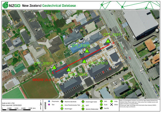
Figure 2.
Site overview and location of five CPT soundings and MASW soundings.
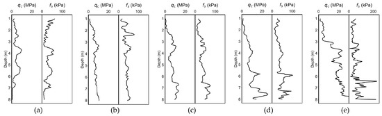
Figure 3.
CPT data: (a) CPT_31917; (b) CPT_31914; (c) CPT_31913; (d) CPT_31918; (e) CPT_31911.
According to the measurement tools in the New Zealand Geotechnical Database, CPT_31911 is offset by 4.70 m from the same cross-section, CPT_31913 is offset by 4.40 m from the same cross-section, CPT_31914 is offset by 4.60 m from the same cross-section, CPT_31917 is offset by 4.75 m from the same cross-section, and CPT_31918 is offset by 4.72 m [43]. According to the results of Xu et al. [24] in using multi-source Bayesian compressive sampling to fuse geotechnical and geophysical data for 2D subsurface site characterization, the effect of local offsets on the fused sampling of subsurface spaces was not significant. In addition, Wang and Li [34] developed an intelligent sampling strategy for multi-stage geotechnical site investigation in planning cross-sections using Voronoi diagrams, BCS, and information entropy, with offset distances within [9.66 m, 14.71 m] for the effective sampling locations measured in the preliminary stages. Therefore, the offsets in this study are within a reasonable range in the projection process. CPT measurement data in Figure 3 has abundant data and data along the depth direction, which can be downloaded from the New Zealand Geotechnical Database [43]. As shown in Figure 4, data are distributed throughout the cross-section at 20 intervals and are used in MSF-BCS. The statistical results of this and data are as follows (Table 1).
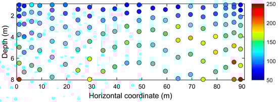
Figure 4.
Vs (m/s) data of MASW along A-A’.

Table 1.
Statistical analysis of
and data.
Geotechnical site characterization is a multi-stage process, and the number and location of initial CPT soundings are typically determined through the engineering experience and expertise of the geotechnical engineer, considering the costs and risks associated with a site-built building and the value of the information. Moreover, when the use of geotechnical site investigations integrated with geophysical techniques is considered in the project, the obtained subsurface space information is increasing, and a reasonable target reliability level is thus defined based on the project cost, time, and the level of project risk. In this paper, the target reliability level is set to 6% and the number of initial CPT soundings based on limited CPT sounding data and geophysical data provided by actual cases in the New Zealand Geotechnical Database in order to implement the data-driven adaptive fusion sampling strategy proposed for demonstration. It is worth noting that this does not indicate a final reliability level of 6%.
In Step 1, for the spatial distribution assessment of liquefaction potential is determined as the threshold for the adaptive fusion sampling strategy process and the initial number of CPT soundings () is determined, and at this time. In Step 2, the CPT-based liquefaction probability assessment framework is used to derive the corresponding sparse data points using the and data from five CPT soundings. The cross-section is then reconstructed from the sparse data using 2D BCS and MCMC. Figure 5 show the mean and standard deviation (SD) of the generated samples, quantifying the uncertainty associated with the reconstruction process, with vertical and horizontal resolutions of 0.125 m and 1 m for the cross-sections, respectively. In Figure 5, the black dashed line indicates the data along the depth direction, and the red solid line indicates the optimal locations C1 and C2 ranges for fusion sampling.
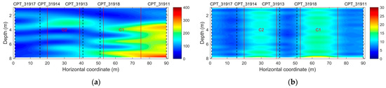
Figure 5.
(qc1N)cs cross-section of five CPT soundings simulated by 2D BCS: (a) Mean; (b) SD.
The data points were interpreted as cross-sections using Equation (2), as shown in Figure 6. Figure 7 shows the interpreted cross-section based on five CPT soundings. The cross-section of the interpreted was generated based on the definition of (Figure 8). A version of the liquefaction probability developed by Ku et al. [25] was used to evaluate the spatial distribution of soil liquefaction potential, as shown in Figure 9. Combined with the consolidation theory in the geotechnical field to monitor liquefaction-induced settlement, Figure 10 illustrates the distribution of the site after liquefaction.
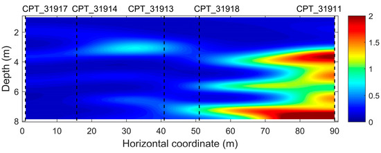
Figure 6.
Interpreted cross-section of CRR based on five CPT soundings.
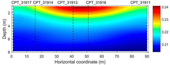
Figure 7.
Interpreted cross-section of CSR based on five CPT soundings.
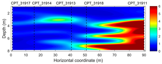
Figure 8.
Interpreted cross-section of FS based on five CPT soundings.
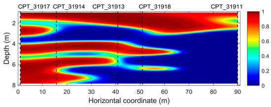
Figure 9.
Interpreted spatial distribution of soil PL (%) based on five CPT soundings.
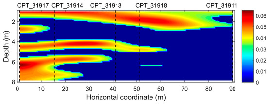
Figure 10.
Interpreted εv distribution of the site based on five CPT soundings.
In Step 3, was obtained from the Step 1–2 process, so one fusion sampling was performed using MSF-BCS to trigger the adaptive process and combined with information entropy theory to determine the optimal location of fusion sampling in the range of C1 and C2. Figure 11 shows the mean and SD of the samples generated after the first fusion sampling at C1. Subsequently, the second fusion sampling was performed at C2, and the sampling was finally stopped with . The sampling process updates the assessment model in a systematic and quantitative manner. Figure 12 shows the mean and SD of the samples generated after fusion sampling at C2. It is worth noting that MSF-BCS is not required since the distances between CPT_31917 and CPT_31914, and between CPT_31913 and CPT_31918 are less than 15 m, satisfying the requirements for generating high-resolution cross sections [20,35].
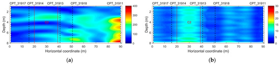
Figure 11.
Simulated high-resolution (qc1N)cs cross-section after the first fusion sampling: (a) Mean; (b) SD.
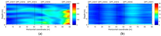
Figure 12.
Simulated high-resolution (qc1N)cs cross-section after the second fusion sampling: (a) Mean; (b) SD.
The best estimates of data at and at are shown in Figure 13a,b, respectively, and the best estimates along the horizontal coordinates are within the 90% confidence interval. Figure 14 shows that the initial reliability level of in the sparse data model is , and after two fusion sampling in a self-adaptive manner, which meets the condition of stopping the fusion sampling. The adaptive fusion sampling process continuously increased the reliability level of the interpreted liquefaction assessment results, and the interpolation uncertainty and soil spatial variability continued to decrease. It is worth noting that additional sampling can be performed using CPT soundings during the multi-stage process of the project when the reliability level does not meet the specific engineering requirements, which is a routine tool in practical engineering [19].
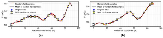
Figure 13.
Best estimates of (qc1N)cs data for 1D cross-section: (a) a1–a2; (b) a3–a4.
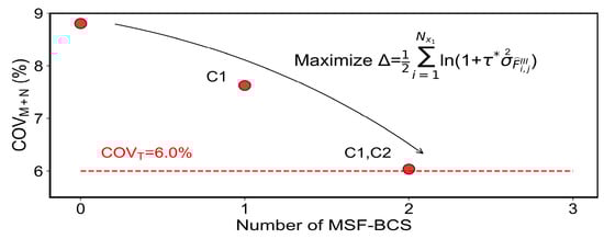
Figure 14.
Variation of COVM+N with the number of MSF-BCS.
The statistical results corresponding to 1D cross-sections a1–a2 and a3–a4 along the horizontal coordinates are shown in Table 2. (qc1N)cs measured values are in the confidence interval range [CI−, CI+] of the computed values of MSF-BCS, which indicates that the proposed strategy is very effective and robust in performing sampling with small computational errors. In addition, the MSF-BCS method retains valuable information about the sampled data, with 90% confidence intervals encompassing most of the local variation in the data and providing a more reasonable average profile.
Table 2.
Statistical analysis of a1–a2 and a3–a4.
In Step 4, a high-resolution cross-section is generated from the data points obtained in Step 3 that achieve the target reliability level, as shown in Figure 15. The corresponding high-resolution cross-sections and spatial distribution of liquefaction potential are subsequently generated, as shown in Figure 16 and Figure 17, respectively. The results indicate that most of the areas of the updated spatial distribution of liquefaction potential would have been liquefied during the earthquake, which is consistent with the liquefaction observed at the field site during the earthquake [44,45]. In addition, the above process verifies the feasibility of the adaptive sampling strategy.
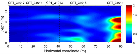
Figure 15.
High-resolution CRR cross-section.
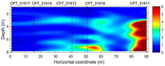
Figure 16.
High-resolution FS cross-section.
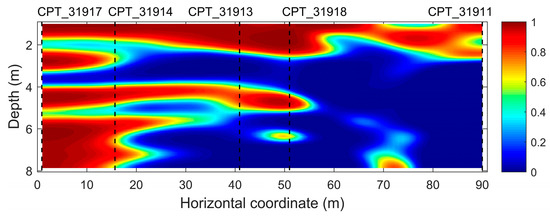
Figure 17.
High-resolution spatial distribution of soil PL (%).
In Step 5, the liquefaction-induced surface settlement monitoring result is updated to quantitatively evaluate the potential for building damage. Figure 18 illustrates the distribution for the subsurface space (A-A’) soil using Equations (1)–(11). The updated was then integrated to estimate the liquefaction-induced , and the monitoring results updated by the adaptive fusion sampling strategy are shown in Figure 19. The results indicate that significant differential settlement occurs at horizontal coordinates 12.9–43.8 m and 50.9–82.0 m. The maximum settlement variations () achieve 81.5 mm and 93.4 mm, respectively, and the estimated after using the adaptive fusion sampling strategy can judge the local area variations more accurately and provide reference for geotechnical engineering design.
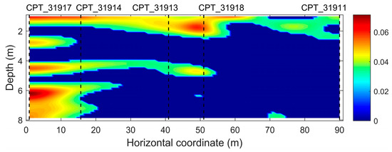
Figure 18.
Updated εv distribution.
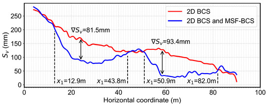
Figure 19.
Comparison of liquefaction-induced Sv monitoring results.
7. Conclusions
This study considers the time, cost, and access constraints of a single geotechnical site investigation. A data-driven adaptive fusion sampling strategy is proposed that automatically develops an assessment model of the spatial distribution of soil liquefaction potential from spatially sparse geotechnical data, performs monitoring of liquefaction-induced settlement, and integrates spatiotemporally unconstrained geophysical data to update the model systematically and quantitatively. It contains three major components: (i) data-driven site modeling by 2D Bayesian compressive sampling using sparse geotechnical data as input, (ii) CPT-based liquefaction procedure incorporating domain knowledge for consolidation settlement modeling, and (iii) multi-source fusion Bayesian compressive sampling coupled with information entropy to automatically fuse sampling samples of geotechnical and geophysical data in a self-adaptive manner and determine the optimal sampling locations.
This strategy yields data combinations with different spatial scales and varying levels of uncertainty, not limited by soil types, to better characterize the subsurface space. Moreover, considering that most current geotechnical engineering models are highly nonlinear and present large data set forms, it is difficult to perform integral solutions in high-dimensional parameter spaces. This study chooses MCMC simulation to obtain the target posterior distribution in MSF-BCS instead of the maximum likelihood estimation in the existing methods. The proposed strategy further obtains information on soil spatial variability while reducing interpolation uncertainty during the performing modeling, illustrated by a real data case from New Zealand.
The results indicate that the developed self-adaptive fusion sampling strategy for evaluating the spatial distribution of soil liquefaction potential and performing monitoring of consolidation settlement, automatically and systematically fusing geophysical data (MASW), effectively overcomes the difficulty of reconstructing the high-resolution spatial distribution of liquefaction potential from sparse geotechnical data, enabling more accurate judgment of settlement variations in local areas, and is an effective tool for site liquefaction hazard analysis.
Although the proposed strategy accurately evaluates the spatial distribution of soil liquefaction potential and performs settlement monitoring, there are still some limitations worth noting. Complex models still require more computational resources and time, thus requiring geotechnical engineers to trade-off between the accuracy of estimation results and computational efficiency. Moreover, MCMC inferring posterior distributions may introduce a reliance on prior distributions, which still require the engineering experience and expertise of geotechnical engineers to determine.
Author Contributions
Conceptualization, H.Y. and Z.L.; methodology, H.Y.; writing—original draft preparation, H.Y.; writing—review and editing, Y.L., Y.Y. and G.T.; funding acquisition, Z.L. All authors have read and agreed to the published version of the manuscript.
Funding
This study was supported by the National Natural Science Foundation of China (41867039), the Guangxi Key Laboratory of Geomechanics and Geotechnical Engineering (20-Y-XT-03), and the Foundation Project of South China Mine Geological Environment Technology Innovation Center (CXZX2020002).
Institutional Review Board Statement
Not applicable.
Informed Consent Statement
Not applicable.
Data Availability Statement
The datasets generated during and/or analyzed during the current study are available from the corresponding author upon reasonable request.
Acknowledgments
The authors acknowledge the members of the New Zealand Geotechnical Database for developing the database.
Conflicts of Interest
The authors declare no conflict of interest.
Notation
| CPT | cone penetration test |
| 2D BCS | two-dimensional Bayesian Compressive Sampling |
| target reliability level | |
| number of CPT soundings | |
| number of fusion samples | |
| cone penetration resistance | |
| equivalent cone penetration resistance in clean sand | |
| sleeve friction | |
| reliability level | |
| sample data | |
| cross-section | |
| cross-section | |
| information gain from fusion sampling | |
| cyclic resistance ratio | |
| cyclic stress ratio | |
| factor of safety | |
| correction factor | |
| normalized cone penetration resistance | |
| soil behavior type index | |
| total vertical stress | |
| effective vertical stress | |
| peak horizontal acceleration at the surface | |
| acceleration of gravity | |
| overburden correction factor | |
| magnitude scaling factor | |
| stress reduction coefficient | |
| soil depth | |
| probability of liquefaction | |
| standard normal cumulative distribution function | |
| liquefaction-induced surface settlement | |
| volume strain | |
| maximum of interest z | |
| maximum cyclic shear strain | |
| relative density of soil | |
| limiting shear strain constraint | |
| matrix represents the 2D data to be characterized | |
| an CPT soundings | |
| ) 2D basis function | |
| -th 2D basis function | |
| an matrix represents a 1D orthonormal basis matrix | |
| an matrix represents a 1D orthonormal basis matrix | |
| measurement matrix specific to this study | |
| common hyperparameter | |
| data to be characterized | |
| data to be characterized | |
| shear wave velocity data obtained by MASW | |
| , respectively | |
| approximation of | |
| a vector represents elements of in a vector format, | |
| likelihood function | |
| prior PDF | |
| approximation of | |
| Kronecker product in linear algebra | |
| an matrix with diagonal elements | |
| reciprocal of unknown variance of the residuals | |
| estimated covariance | |
| a modified Bessel function of the second type with parameter | |
| union of the non-trivial 2D basis functions | |
| estimated covariance | |
| estimated covariance | |
References
- Wang, Y.; Fu, C.; Huang, K. Probabilistic Assessment of Liquefiable Soil Thickness Considering Spatial Variability and Model and Parameter Uncertainties. Géotechnique 2017, 67, 228–241. [Google Scholar] [CrossRef]
- Chen, Q.; Wang, C.; Juang, C.H. Probabilistic and Spatial Assessment of Liquefaction-Induced Settlements through Multiscale Random Field Models. Eng. Geol. 2016, 211, 135–149. [Google Scholar] [CrossRef]
- Seed, H.B.; Idriss, I.M. Simplified Procedure for Evaluating Soil Liquefaction Potential. J. Soil Mech. Found. Div. 1971, 97, 1249–1273. [Google Scholar] [CrossRef]
- Schmidt, J.; Moss, R. Bayesian Hierarchical and Measurement Uncertainty Model Building for Liquefaction Triggering Assessment. Comput. Geotech. 2021, 132, 103963. [Google Scholar] [CrossRef]
- Boulanger, R.W.; Idriss, I.M. CPT-Based Liquefaction Triggering Procedure. J. Geotech. Geoenviron. Eng. 2016, 142, 04015065. [Google Scholar] [CrossRef]
- Juang, C.H.; Ching, J.; Wang, L.; Khoshnevisan, S.; Ku, C.-S. Simplified Procedure for Estimation of Liquefaction-Induced Settlement and Site-Specific Probabilistic Settlement Exceedance Curve Using Cone Penetration Test (CPT). Can. Geotech. J. 2013, 50, 1055–1066. [Google Scholar] [CrossRef]
- Wang, Y.; Au, S.-K.; Cao, Z. Bayesian Approach for Probabilistic Characterization of Sand Friction Angles. Eng. Geol. 2010, 114, 354–363. [Google Scholar] [CrossRef]
- Cao, Z.; Wang, Y. Bayesian Model Comparison and Selection of Spatial Correlation Functions for Soil Parameters. Struct. Saf. 2014, 49, 10–17. [Google Scholar] [CrossRef]
- Juang, C.H.; Zhang, J.; Shen, M.; Hu, J. Probabilistic Methods for Unified Treatment of Geotechnical and Geological Uncertainties in a Geotechnical Analysis. Eng. Geol. 2019, 249, 148–161. [Google Scholar] [CrossRef]
- Yang, H.; Liu, Z.; Li, Y.; Wei, H.; Huang, N. CatBoost–Bayesian Hybrid Model Adaptively Coupled with Modified Theoretical Equations for Estimating the Undrained Shear Strength of Clay. Appl. Sci. 2023, 13, 5418. [Google Scholar] [CrossRef]
- Zhao, Z.; Duan, W.; Cai, G.; Wu, M.; Liu, S. CPT-Based Fully Probabilistic Seismic Liquefaction Potential Assessment to Reduce Uncertainty: Integrating XGBoost Algorithm with Bayesian Theorem. Comput. Geotech. 2022, 149, 104868. [Google Scholar] [CrossRef]
- Guan, Z.; Wang, Y.; Stuedlein, A.W. Efficient Three-Dimensional Soil Liquefaction Potential and Reconsolidation Settlement Assessment from Limited CPTs Considering Spatial Variability. Soil Dyn. Earthq. Eng. 2022, 163, 107518. [Google Scholar] [CrossRef]
- Tian, H.; Wang, Y. Data-Driven and Physics-Informed Bayesian Learning of Spatiotemporally Varying Consolidation Settlement from Sparse Site Investigation and Settlement Monitoring Data. Comput. Geotech. 2023, 157, 105328. [Google Scholar] [CrossRef]
- Ji, S.; Xue, Y.; Carin, L. Bayesian Compressive Sensing. IEEE Trans. Signal Process. 2008, 56, 2346–2356. [Google Scholar] [CrossRef]
- Guan, Z.; Wang, Y. CPT-Based Probabilistic Liquefaction Assessment Considering Soil Spatial Variability, Interpolation Uncertainty and Model Uncertainty. Comput. Geotech. 2022, 141, 104504. [Google Scholar] [CrossRef]
- Guan, Z.; Wang, Y. SPT-Based Probabilistic Evaluation of Soil Liquefaction Potential Considering Design Life of Civil Infrastructures. Comput. Geotech. 2022, 148, 104807. [Google Scholar] [CrossRef]
- Guan, Z.; Wang, Y.; Zhao, T. Delineating the Spatial Distribution of Soil Liquefaction Potential in a Cross-Section from Limited Cone Penetration Tests. Soil Dyn. Earthq. Eng. 2021, 145, 106710. [Google Scholar] [CrossRef]
- Guan, Z.; Wang, Y. Assessment of Liquefaction-Induced Differential Ground Settlement and Lateral Displacement Using Standard Penetration Tests with Consideration of Soil Spatial Variability. J. Geotech. Geoenviron. Eng. 2022, 148, 04022018. [Google Scholar] [CrossRef]
- Zhao, T.; Wang, Y.; Xu, L. Efficient CPT Locations for Characterizing Spatial Variability of Soil Properties within a Multilayer Vertical Cross-Section Using Information Entropy and Bayesian Compressive Sensing. Comput. Geotech. 2021, 137, 104260. [Google Scholar] [CrossRef]
- Guan, Z.; Wang, Y.; Zhao, T. Adaptive Sampling Strategy for Characterizing Spatial Distribution of Soil Liquefaction Potential Using Cone Penetration Test. J. Rock Mech. Geotech. Eng. 2022, 14, 1221–1231. [Google Scholar] [CrossRef]
- Montgomery, J.; Boulanger, R.W. Effects of Spatial Variability on Liquefaction-Induced Settlement and Lateral Spreading. J. Geotech. Geoenviron. Eng. 2017, 143, 04016086. [Google Scholar] [CrossRef]
- Huang, J.; Zheng, D.; Li, D.-Q.; Kelly, R.; Sloan, S.W. Probabilistic Characterization of Two-Dimensional Soil Profile by Integrating Cone Penetration Test (CPT) with Multi-Channel Analysis of Surface Wave (MASW) Data. Can. Geotech. J. 2018, 55, 1168–1181. [Google Scholar] [CrossRef]
- Adewoyin, O.; Joshua, E.; Akinwumi, I.; Maxwell, O.; Joel, E. Evaluation of Geotechnical Parameters Using Geophysical Data. J. Eng. Technol. Sci. 2017, 49, 95–113. [Google Scholar] [CrossRef]
- Xu, J.; Wang, Y.; Zhang, L. Fusion of Geotechnical and Geophysical Data for 2D Subsurface Site Characterization Using Multi-Source Bayesian Compressive Sampling. Can. Geotech. J. 2022, 59, 1756–1773. [Google Scholar] [CrossRef]
- Ku, C.-S.; Juang, C.H.; Chang, C.-W.; Ching, J. Probabilistic Version of the Robertson and Wride Method for Liquefaction Evaluation: Development and Application. Can. Geotech. J. 2012, 49, 27–44. [Google Scholar] [CrossRef]
- Robertson, P.K.; Wride, C. (Fear) Evaluating Cyclic Liquefaction Potential Using the Cone Penetration Test. Can. Geotech. J. 1998, 35, 442–459. [Google Scholar] [CrossRef]
- Robertson, P. Performance Based Earthquake Design Using the CPT. In Proceedings of the International Conference on Performance-Based Design in Earthquake, Tokyo, Japan, 25 May 2009; pp. 3–20. [Google Scholar]
- Youd, T.L.; Idriss, I.M. Liquefaction Resistance of Soils: Summary Report from the 1996 NCEER and 1998 NCEER/NSF Workshops on Evaluation of Liquefaction Resistance of Soils. J. Geotech. Geoenviron. Eng. 2001, 127, 297–313. [Google Scholar] [CrossRef]
- Duan, W.; Zhao, Z.; Cai, G.; Pu, S.; Liu, S.; Dong, X. Evaluating Model Uncertainty of an in Situ State Parameter-Based Simplified Method for Reliability Analysis of Liquefaction Potential. Comput. Geotech. 2022, 151, 104957. [Google Scholar] [CrossRef]
- Zhang, G.; Robertson, P.K.; Brachman, R.W.I. Estimating Liquefaction-Induced Lateral Displacements Using the Standard Penetration Test or Cone Penetration Test. J. Geotech. Geoenviron. Eng. 2004, 130, 861–871. [Google Scholar] [CrossRef]
- Ishihara, K.; Yoshimine, M. Evaluation of Settlements in Sand Deposits Following Liquefaction During Earthquakes. Soils Found. 1992, 32, 173–188. [Google Scholar] [CrossRef]
- Idriss, I.M.; Boulanger, R.W. Soil Liquefaction during Earthquakes; Earthquake Engineering Research Institute: Oakland, CA, USA, 2008; p. 136. [Google Scholar]
- Zhao, T.; Hu, Y.; Wang, Y. Statistical Interpretation of Spatially Varying 2D Geo-Data from Sparse Measurements Using Bayesian Compressive Sampling. Eng. Geol. 2018, 246, 162–175. [Google Scholar] [CrossRef]
- Wang, Y.; Li, P. Data-Driven Determination of Sample Number and Efficient Sampling Locations for Geotechnical Site Investigation of a Cross-Section Using Voronoi Diagram and Bayesian Compressive Sampling. Comput. Geotech. 2021, 130, 103898. [Google Scholar] [CrossRef]
- Zhao, T.; Xu, L.; Wang, Y. Fast Non-Parametric Simulation of 2D Multi-Layer Cone Penetration Test (CPT) Data without Pre-Stratification Using Markov Chain Monte Carlo Simulation. Eng. Geol. 2020, 273, 105670. [Google Scholar] [CrossRef]
- Tipping, M.E. Sparse Bayesian Learning and the Relevance Vector Machine. J. Mach. Learn. Res. 2001, 1, 211–244. [Google Scholar] [CrossRef]
- Yang, H.-Q.; Zhang, L.; Xue, J.; Zhang, J.; Li, X. Unsaturated Soil Slope Characterization with Karhunen–Loève and Polynomial Chaos via Bayesian Approach. Eng. Comput. 2019, 35, 337–350. [Google Scholar] [CrossRef]
- Long, M.; Trafford, A.; McGrath, T.; O’Connor, P. Multichannel Analysis of Surface Waves (MASW) for Offshore Geotechnical Investigations. Eng. Geol. 2020, 272, 105649. [Google Scholar] [CrossRef]
- Yang, H.-Q.; Zhang, L.; Pan, Q.; Phoon, K.-K.; Shen, Z. Bayesian Estimation of Spatially Varying Soil Parameters with Spatiotemporal Monitoring Data. Acta Geotech. 2021, 16, 263–278. [Google Scholar] [CrossRef]
- Liu, J.; Wu, Q.; Amin, M.G. Multi-Task Bayesian Compressive Sensing Exploiting Signal Structures. Signal Process. 2021, 178, 107804. [Google Scholar] [CrossRef]
- Shannon, C.E. A Mathematical Theory of Communication. Bell Syst. Tech. J. 1948, 27, 623–656. [Google Scholar] [CrossRef]
- Zhao, T.; Wang, Y. Determination of Efficient Sampling Locations in Geotechnical Site Characterization Using Information Entropy and Bayesian Compressive Sampling. Can. Geotech. J. 2019, 56, 1622–1637. [Google Scholar] [CrossRef]
- NZGD. New Zealand Geotechnical Database. Available online: https://www.nzgd.org.nz/ (accessed on 26 June 2022).
- Bray, J.; Cubrinovski, M.; Zupan, J.; Taylor, M. Liquefaction Effects on Buildings in the Central Business District of Christchurch. Earthq. Spectra 2014, 30, 85–109. [Google Scholar] [CrossRef]
- Bradley, B.A. Site-Specific and Spatially-Distributed Ground-Motion Intensity Estimation in the 2010–2011 Canterbury Earthquakes. Soil Dyn. Earthq. Eng. 2014, 61–62, 83–91. [Google Scholar] [CrossRef]


Disclaimer/Publisher’s Note: The statements, opinions and data contained in all publications are solely those of the individual author(s) and contributor(s) and not of MDPI and/or the editor(s). MDPI and/or the editor(s) disclaim responsibility for any injury to people or property resulting from any ideas, methods, instructions or products referred to in the content. |
© 2023 by the authors. Licensee MDPI, Basel, Switzerland. This article is an open access article distributed under the terms and conditions of the Creative Commons Attribution (CC BY) license (https://creativecommons.org/licenses/by/4.0/).