Offloading Strategy of Multi-Service and Multi-User Edge Computing in Internet of Vehicles

Abstract

An edge computing offloading strategy was proposed with the goal of addressing the issue of low edge computing efficiency and service quality in the multi-service and multi-user intersections of networked vehicles. This strategy took into account all relevant factors, including the matching of users and service nodes, offloading ratio, bandwidth and computing power resource allocation, and system energy consumption. It is mainly divided into 2 tasks: (1) Service node selection: A fuzzy logic-based service node selection algorithm (SNFLC) is proposed. The linear equation for node performance value is determined through fuzzy reasoning by specifying three performance indexes as input. Gradient descent method is used to find the optimal value of the objective function, and the Lyapunov criterion coefficient is introduced to improve the stability of the algorithm. (2) Offload ratio and resource allocation are solved: The coupling between offload ratio and bandwidth resource allocation is confirmed by relaxing integer variables because the optimization goal problem is a NP problem, and the issue is divided into two sub-problems. At the same time, a low-complexity alternate iteration resource allocation algorithm (LC-IRA) is proposed to solve the bandwidth resource and computational power resource allocation. According to simulation results, the performance of genetic ant colony algorithm (G_ACA), non orthogonal multiple access technology (NOMA) and LC-IRA are improved by 26.5%, 31.37%, and 45.52%, respectively, compared with the random unloading allocation (RUA) and average distribution (AD).

1. Introduction

As a key technology to promote the development of the fifth generation (5G) network, mobile edge computing (MEC) extends computing, communication, and storage facilities to the edge of the network [1]. By offering low-latency local computing resources, it can facilitate novel mobile applications (augmented reality, virtual reality, autonomous driving, etc.). In order to offer users effective services, new 5/6G applications also depend on computational offloading technology. There are many useful technologies and methods that have been developed as a result of extensive research in both industry and academics on computational offloading techniques in MEC networks [2]. Edge computing has developed into a promising computing platform supporting computationally intensive and delay-sensitive mobile applications, and it is also widely used in the field of connected vehicles. The development of the intelligent connected vehicle (ICV) requires the sharing and collaboration of cars, roads, internet, and the cloud, and deployment of the car networking platform, roadside units (RSUs) and roadside infrastructure, terminal sensors, etc. In addition, it needs to realize the car and car, car and road, and car and people interactions in all kinds of application scenarios. For example, the vehicle density on the roadside infrastructure of crossroads is complex and needs to consider many factors, especially the multi-edge service and multi-user scenarios.

However, due to the limited coverage of edge computing resources and services, there are still some key problems to be properly solved, especially the edge resource allocation. In this context, mobile users are permitted to delegate work to service nodes, and the MEC server chooses which users will receive data and computing power resources. It is also necessary to consider whether the allocation problem is coupled with the requirements of a user write-offload ratio or a quality of service. Therefore, one of the main challenges is how to distribute resources wisely and choose the best service nodes for networked vehicles.

Edge computing can complete data processing tasks independently and quickly in the field, and edge computing can process data independently in the local area, so as to meet the high real-time requirements in the field of traffic. In a specific scenario, the communication link adapts to the change because the topological structure of different internet of vehicles scenarios varies. This change is too great for the fixed transmission rate model that is currently in use. There is also a lack of collaboration between vehicles and service nodes, which results in low utilization of edge computing resources. For this reason, the research on task unloading of on-board edge computing should address the following challenges: (1) Adaptive unloading strategies combined with traffic density are not taken into account when analyzing the uneven distribution of road hotspots brought on by changes in traffic density. (2) To increase the resource utilization of edge nodes, the multi-objective optimization issue in on-board edge computing must consider the selection of service nodes, the reasonable allocation of bandwidth, and computing resources. This paper studies the issue of computing task offloading in the intersection scene under the inter-office voucher (IOV) environment so as to solve the problems mentioned as before.

As a result, this paper studies the vehicle computing task unloading problem in the intersection scenario; carefully considers the matching between users and service nodes, unloading ratio, bandwidth, and computing resource allocation; and establishes the optimization target of minimizing system energy consumption. The proper matching between users and service nodes can reduce many unnecessary expenses for subsequent uninstallation. At the same time, the bandwidth resource in communication is taken as a variable to verify the coupling between this variable and the unloading ratio. Finally, a related algorithm to minimize system energy consumption is proposed, and based on Matlab, and the design and simulation of the networked vehicle system scene are carried out to verify the effectiveness of the proposed algorithm and strategy.

2. Related Work

With its ability to be used in both edge and end applications and its features of low latency and high reliability, mobile edge computing is a widely adopted computing paradigm. MEC’s core principle is the local processing of mobile application data at the network edge, close to the end user, or performing computation tasks (using, for example, a wireless network controller, a long term evolution (LTE) macro station, a small cell micro base station, etc.). As a result, the end-to-end delay is reduced and the resource scarcity of mobile devices is lessened. The MEC ecosystem still faces a number of significant issues that have not yet been adequately addressed as an emerging computing paradigm, and task offloading is just one of the difficulties in these areas. In order to achieve the best operational performance of the application and make efficient use of MEC resources, it is crucial to choose the appropriate task to offload to the appropriate MEC server at the appropriate moment [3].

Reference [4] proposed the network slicing and load balancing algorithm (VECSlicLB). The algorithm virtualizes the data plane of edge nodes by using the network slicing function. VECSlicLB algorithm is based on the decoupling of the control plane and the data plane to realize load balancing among edge nodes and improve resource utilization of edge nodes. A heuristic algorithm called Horae is suggested in the literature [5] when scheduling jobs for various users with precedence and geographic restrictions. However, it is simple for this heuristic method to enter a local optimum. Its shortcomings will shortly be made clear if it is used for multi-objective optimization in challenging situations such as those related to the internet of vehicles (IOV). In order to reduce the overall delay of all tasks, studies have been conducted on joint resource allocation and other optimization variables, including joint server allocation, transmission power allocation between users and MEC servers, MEC server computing resource allocation, time allocation, and channel allocation [6]. The fractional search method is optimized for computing resource allocation, but the authors do not take into account a coupling relationship between the offloading ratio and these resource allocations, and directly idealize it as a separate variable [7,8,9,10,11]. In reference [12], an effective low-complexity heuristic algorithm is proposed for a multi-user MEC supported wireless communication system to maximize the number of offloading tasks for all uses in uplink communication while maintaining the computing resources of MEC at an acceptable level. The proposed resource allocation strategy cannot ensure the rationality of the allocation, and this algorithm is established to increase the number of user tasks that are offloaded. Nevertheless, this algorithm offers a nearly optimal solution with little time overhead. With regard to the matching issue, the literature [13] considers the incentives for using the idle computing resources of vehicles as the edge nodes, and attempts to establish a differential pricing model based on different resource states. A gradient-based iterative resource allocation method (GRAIA) is developed. The issue of matching users and vehicles is then considered. An enhanced hierarchical clustering algorithm (HDBSACAN) is suggested in reference [14]. To locate suitable service vehicles for use as task vehicles and to increase task unloading effectiveness, an evaluation expression for nearby service vehicles is proposed. The literature [15] takes into account computing and communication resource allocation in conjunction with communication efficiency, combining delay and energy consumption to reduce overall network overhead. The issue is broken down into three smaller issues that are each solved separately using mathematical techniques, but this approach is very computationally complicated. In order to investigate the resource allocation issue in the internet of things (IoT) and significantly enhance the performance of wireless communication, the literature [16] also considers the energy cost and processing delay of wireless transmission and computation. However, this research also disregards the possibility of a coupling between the offloading ratio and resources. A joint user selection and resource allocation algorithm is suggested in the literature [17] to optimize user energy efficiency, which is calculated as the relationship between user throughput and energy usage. The user’s offloading of selection and uplink transmission power are included in the formulation of the energy efficiency maximization issue as a mixed integer score nonlinear optimization problem [18]. The problem is transformed into an equivalent subtractive convex optimization problem through the relaxation transformation method, and the corresponding optimal solutions of user selection and power allocation are provided [19].

The complex connected vehicle scenario at the intersection is examined in this paper. Researchers thoroughly evaluate the matching between users and service nodes, offloading ratio, bandwidth, and computing power resource allocation, and propose the optimization target of reducing system energy consumption. There are mainly two innovations: on the one hand, the innovation of dynamic matching between vehicles and service nodes; on the other hand, the innovation of the vehicle task unloading problem. The appropriate matching between users and service nodes can cut down many unnecessary costs for subsequent offloading [20].

3. Optimization of Vehicle Edge System Model

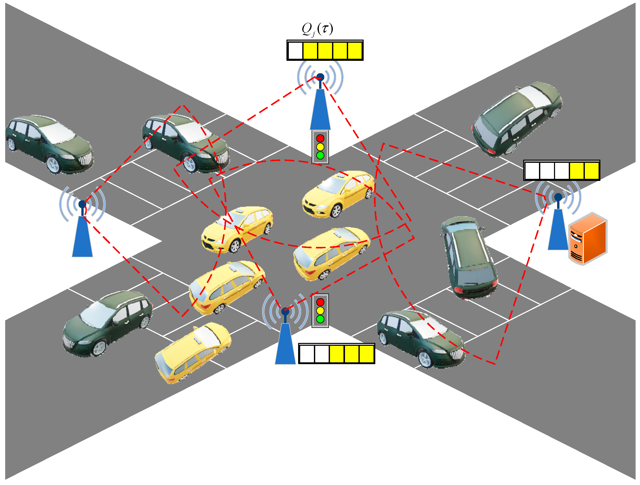
3.1. System Model

As shown in Figure 1, the intersection scene is built up with vehicle sets $\mathrm{V}=(v_1,v_2,\dots ,v_N)$ and RSU and $\mathrm{R}=(R_1,R_2,\dots ,R_J)$, and the time is discrete into a single observable time $t=(1,2,\dots ,\tau )$ slot with the length of $\Delta =\frac{t}{\tau }$. The RSU configuration interval is brief in the intersection situation. Only one MEC server is needed for vehicle job calculation and processing in order to prevent resource waste. The tasks carried by each vehicle can be simplified into a binary form $Tas{k}_{vi}=\{S_{vi},T_{vi}^{max}\},i\in (1,N)$, which respectively describes the vehicle task data size and the maximum allowable delay. Some duties must be delegated to an edge server with high processing capacity due to the vehicle’s limited computing capabilities, so the task computation uses a binary representation. If tasks are unloaded simultaneously onto the MEC server while there is heavy traffic flow at the intersection, the machine will become overloaded and eventually fail. Therefore, the task queue model is created based on the randomness of tasks. Tasks in the system are randomly generated and delivered to a specific RSU. After the storage period, the tasks are migrated to the MEC server for calculation. The task queue length on any RSU is $Q_j(\tau )(j\in J)$, and it is updated according to the following equation:

$$Q_j(\tau +1)=max(Q_j(\tau )-W_j(\tau ),0)+U_j(\tau )$$

(1)

$W_j(\tau )$ is a task that has been migrated, while $U_j(\tau )$ indicates that the task has been received. It is set so that when the RSU task buffer exceeds the threshold $Q_{max}$, the vehicle is no longer permitted to place tasks.

(1)

Local Computation

The vehicle itself has a certain amount of computing resources, but because there are only so many of them, it can only handle a certain amount of computational work. Then, the number of CPU cycles allocated for the local computing task can be described as:

$$Cycl{e}_{vi}=\sqrt{\frac{{\Gamma }_{vi}^{local}}{\Phi (1-\eta )S_{vi}^{local}}}$$

(2)

where the computing capability of the ${\Gamma }_{vi}^{local}$ vehicle is $v_i$, $\Phi$ represents the effective constant of the capacitor switch of the vehicle, $S_{vi}^{local}=(1-a_{vi}^{\tau })S_{vi}$ is the number of tasks that the vehicle needs to compute locally, and $a_{vi}^{\tau }$ refers to the unloading scale factor. The following summarizes the local execution duration and energy usage:

$$T_{vi}^{local}=\frac{(1-\eta )S_{vi}^{local}}{Cycl{e}_{vi}}$$

(3)

$$E_{vi}^{local}=k{({\Gamma }_{vi}^{local})}^2(1-a_{vi}^{\tau })S_{vi}$$

(4)

$k$ depends on the energy coefficient of the chip structure.

(2)

Unloading calculation

During the uninstall process, the delay is divided into uplink transmission delay, waiting delay, and calculation delay (the transmission time between the MEC server and the RSU and the task result sending time are ignored). According to the relationship between the limit data transmission rate and bandwidth in a noisy channel (Shannon’s theorem), the transmission rate between the vehicle and the RSU is defined as:

$$r_{vi,j}^{un}=B_{vi}{\log }_2(1+\frac{p_{vi,j}^{un}{\mathrm{H}}_{vi,j}}{{\mathrm{O}}^2})$$

(5)

where, $B_{vi}$ represents the bandwidth resource allocated by the system to the vehicle $vi$, $p_{vi,j}^{un}$ represents the channel transmission power, ${\mathrm{H}}_{vi,j}(\tau )$ is the standard channel vector between the vehicle and the RSU, and $\mathrm{O}$ represents the white Gaussian noise. The transmission delay generated by the unloading process is expressed as $T_{vi,j}^{un}=\frac{\eta S_{vi}^{un}}{r_{vi,j}^{un}(\tau )}$, energy consumption generated $E_{vi,j}^{un}=p_{vi,j}^{un}*T_{vi,j}^{un}$, $S_{vi,j}^{un}=a_{vi}^{\tau }{S}_{vi}$ represents the number of tasks unloaded by the vehicle $vi$ to the RSU $j$, and $p_{vi,j}^{un}$ is the transmission power. When tasks are assigned to the RSU, they are migrated to the MEC server following the queue in serial processing mode. The waiting time is:

$$T_{vi,j}^{wait}(\tau )=\frac{Q_j(\tau )-Q_j(\tau -1)}{{\Gamma }_{mec}}$$

(6)

(${\Gamma }_{mec}$ is the computing capacity of the MEC server). After the migration to the MEC server, the computation time and energy consumption are expressed as $T_{vi,j}^{cal}=\frac{S_{vi}^{un}}{{\Gamma }_{mec}}$, $E_{mec}^{cal}=\varpi *{(P_{vi})}^3$. $P_{vi}$ is the computation power allocated by the MEC server to the task of the vehicle.

3.2. Optimization Model

The vehicle task is configured so that it cannot be fully locally computed or fully unloaded while still meeting the user’s requirements for service quality. To put it another way, the scale factor is dynamically adjusted to accommodate the task’s dynamic unloading, and the numerical relation is $0<a_{vi}^{\tau }<1$. At the same time, in order to reduce the energy consumption of the system, before the load task processing, the vehicle in the system is matched to the appropriate service node, the matching vector is introduced $V_i^j=[V_1^j,V_2^j,\dots ,V_N^j](\tau )$, and the element $V_N^j$ is the vehicle $i$ selection to unload part of the task to the node $j$.

The total system energy consumption includes the local computing energy consumption, transmission energy consumption, and computing energy consumption, which can be expressed as $e=E_{vi}^{local}+E_{vi,j}^{un}+E_{mec}^{cal}$. In short, an optimization model is developed to minimize the system’s overall energy usage, as illustrated below.

$$\begin{array}{ll}\mathrm{P}1 & \underset{\{V_i^j,a_{vi}^{\tau },P_{vi},B_{vi}\}}{min} e\\ s.t & \\ & max\{T_{vi}^{local},T_{vi,j}^{un}+T_{vi,j}^{wait}(\tau )+T_{vi,j}^{cal}\}\le T_{vi}^{max}\hfill & \left(7\mathrm{a}\right) \\ & \hfill Q_j(\tau )\le Q_{max} ,\forall j\in J\hfill & \left(7\mathrm{b}\right) \\ & \hfill B_{vi}>0,\forall vi\in N\hfill & \left(7\mathrm{c}\right) \\ & \hfill {\displaystyle \sum _{vi=1}^N{B}_{vi}\le B_{max}}\hfill & \left(7\mathrm{d}\right) \\ & \hfill 0<a_{vi}^{\tau }<1\hfill & \left(7\mathrm{e}\right) \\ & \hfill P_{vi}>0,\forall vi\in N\hfill & \left(7\mathrm{f}\right) \\ & \hfill {\displaystyle \sum _{vi=1}^{vN}{P}_{vi}}\le P_{max}\hfill & \left(7\mathrm{g}\right) \\ & \hfill \eta =\{0,1\}\hfill & \left(7\mathrm{h}\right) \end{array}$$

(7)

Constraint (a) ensures that the task processing time stays within the maximum allowable delay; constraint (b) ensures load balancing, and the backlog of each node cannot exceed the maximum threshold $Q_{max}$. Constraints (c), (d), (f), and (g) stipulate that the bandwidth and computing power allocated by the server to the user cannot surpass its own maximum threshold $B_{max},P_{max}$. Constraint (e) guarantees the requirements of the unloading ratio on the premise of satisfying the quality of service; constraint (h) represents two unloading instructions.

4. Edge Computing Offloading Method in Internet of Vehicles

Due to the complex topology of the connected vehicles scenario, the same vehicle may appear in the service scope of multiple RSUs at the same time. The system’s vehicles and RSU must be correctly matched in order to prevent network congestion brought on by multiple users connecting to the same RSU at once. In addition, radio resources are shared via virtualization among users with different resource needs due to MEC’s strong computing and storage capabilities. After completing system matching, the server provides bandwidth and computing power resources for users. Therefore, this section will be divided into two stages to achieve the final system optimization.

Definition 1.

Edge service node selection: The fuzzy logic system is established, and the vehicle-related performance metrics are input to evaluate each service node. Finally, the evaluation result vector is output, and the finest service node is located at the location of the vector’s maximum value. (Definitions 1 and Definitions 2 are sourced from reference [1]).

Definition 2.

Offload ratio and resource allocation: Following system matching, the optimization goals are accomplished by modifying the unloading ratio and judicious distribution of resources (power and bandwidth).

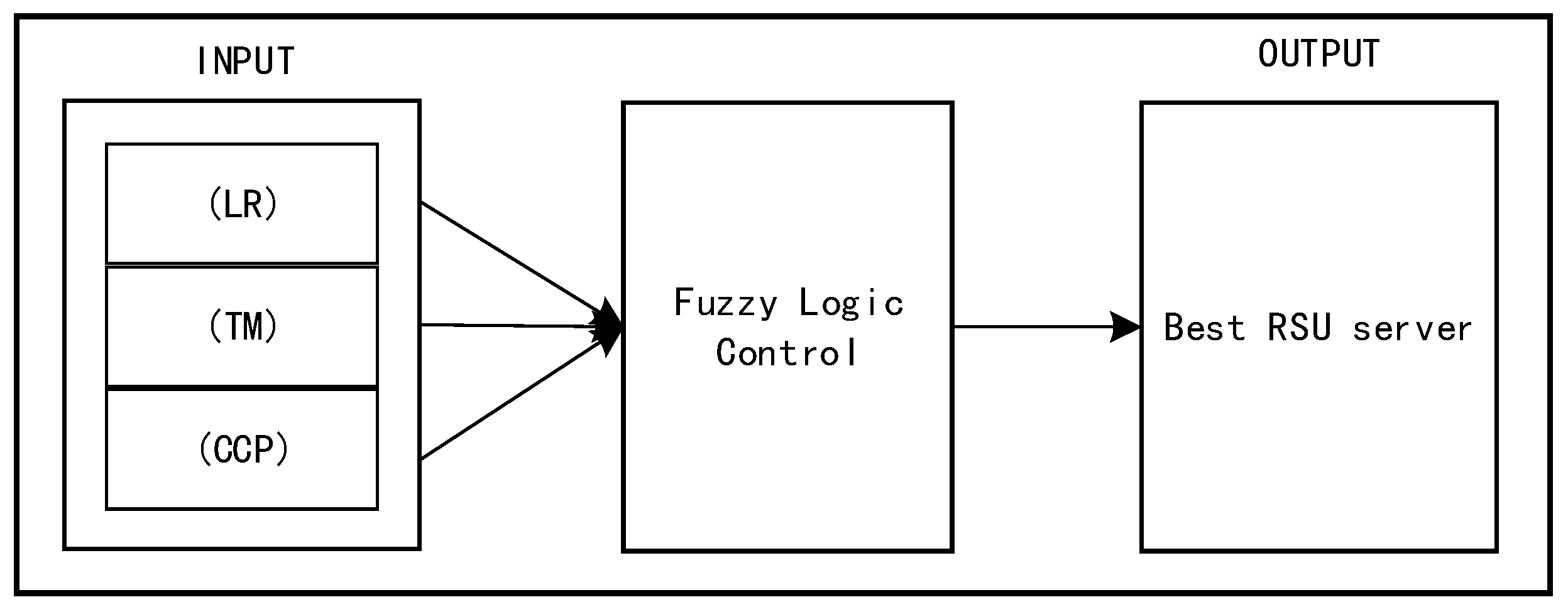
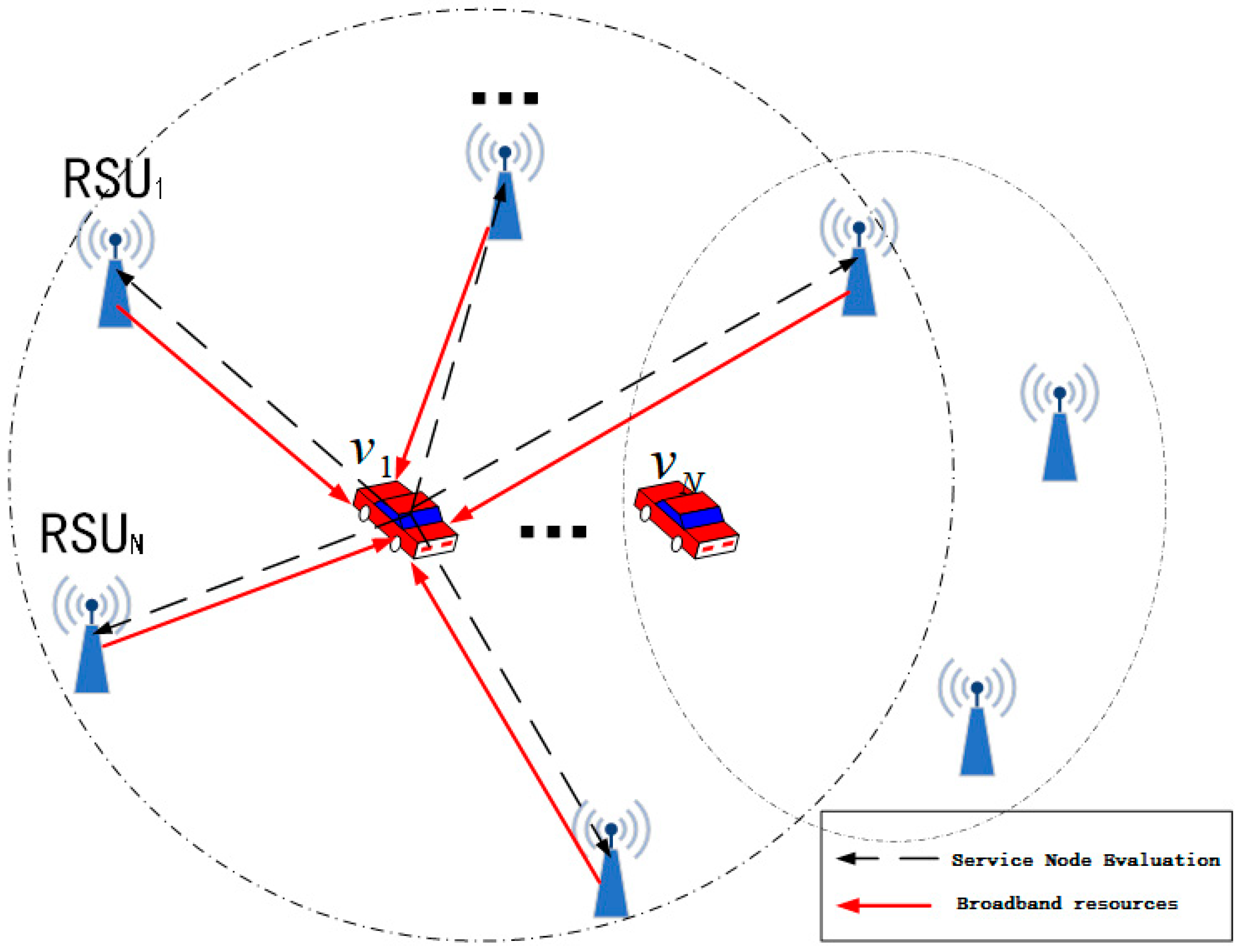
4.1. Edge Service Node Selection

Fuzzy control is an intelligent control method based on fuzzy set theory, fuzzy language variables, and fuzzy logic reasoning. It is an intelligent control algorithm that imitates human fuzzy reasoning and decision-making process in behavior. In fuzzy control, the experience of operators or experts are composed of fuzzy rules, and then the real-time signals from sensors are fuzziness; the fuzziness signals are used as the input of the fuzzy rules to complete fuzzy inference, and the output obtained after inference is added to the actuator. Fuzzy inference systems include both Mamdani and Sugeno models, both of which are used to achieve decision processing in complex systems. The latter has high complexity but little performance improvement, making it not the best choice for fuzzy inference. Therefore, a service node selection algorithm based on the fuzzy logic control principle (SNFLC) is suggested in this part, and its structure is shown in Figure 2.

Load ratio (LR) determines whether it has enough room to store vehicle tasks. By introducing the three indicators, task mobility (TM) depicts the node’s task-forwarding effectiveness, continuous connectivity probability (CCP) gauges the node’s dependability, and performance of the service node (PSN) is determined, as shown in Figure 3. It is important to note that the network architecture of the internet of vehicles is constantly evolving. The topology structure is assumed to be constant throughout each time slot segment in order to efficiently complete the duties that come after.

(1)

LR

Load ratio describes the load balance of RSU at a certain time slot $\tau$. The load ratio at any node is defined by the task queue length $Q(\tau )$ and cache capacity threshold $Q_{\mathit{max}}$ of the time slot $\tau$. The expression (8) shows that the smaller the load ratio is, the larger the remaining storage space is, and the more likely it is to successfully store vehicle tasks.

$$L{R}_j(\tau )=\frac{Q_j(\tau )}{Q_{\max }}$$

(8)

(2)

TM

Vehicle tasks arrive at the service node in the form of data packets, and task mobility is a metric to measure the task processing rate of the node. The larger the mobility rate, the faster the task can be migrated to the MEC server for processing. The task arrival rate can be represented by using the sliding exponential average algorithm to mimic the packet arrival rate $Arrive(\tau )$.

$$Arrive(\tau )=\frac{dQ(\tau )(1{-\mathrm{e}}^{-\Delta /\wp })}{\Delta }+{\mathrm{e}}^{-\Delta /\wp }Arrive(\tau -1)$$

(9)

where $\wp$ is a constant, reflecting the correlation between the arrival rate of the task before and after and the time. Usually, the value of ${\mathrm{e}}^{-\Delta /\wp }$ is 0.1, which is used to represent the instantaneous rate. $dQ(\tau )=Q(\tau )-Q(\tau -1)$ indicates the number of tasks that reach the node in a time slot $\tau$. $Service(\tau )$ is the node forwarding service rate, so the task migration rate can be expressed as the ratio of the two.

$$Tra{n}_j(\tau )=Arrive(\tau )/Service(\tau )$$

(10)

(3)

CCP

The benchmark used to assess the node’s dependability is the constant connection probability between the vehicle and the node. The higher the probability is, the longer the connection will not be forced to terminate the task due to the signal terminal, and the connection will always exist until the end of the task processing. The Poisson distribution with density as $\ell$ is satisfied by the system’s car distribution. On a road with as area denoted as $\mathrm{A}$, the number of vehicles is a Poisson random variable. Therefore, the probability of having $N$ vehicle on this road section is:

$$f(N,A)=\frac{\ell {\mathrm{A}}^N}{e^{\ell \mathrm{A}}N!},N\ge 0$$

(11)

$$p_{vi}^j=1-(1-{\mathrm{K}}_{vi}^j)(1-{\mathrm{K}}_{vi}^j(•))$$

(12)

${\mathrm{K}}_{vi}^j$ is the connection probability of the vehicle $i$ directly connecting to the RSU $j$, and ${\mathrm{K}}_{vi}^j(•)$ is the continuous connection probability of the vehicle directly connecting to the RSU (namely, the connectivity stability of the two). On the contrary, the probability that the vehicle fails to connect to the RSU or fails to continuously connect after establishing the connection are $1-{\mathrm{K}}_{vi}^j$ and $1-{\mathrm{K}}_{vi}^j(•)$, respectively. A vehicle’s likelihood of connecting to the RSU is unaffected by whether another vehicle is connected to the RSU due to the strong transceiver power of the RSU, meaning that the connection establishment process is entirely rational. Therefore, the probability that the vehicle is directly connected to the RSU is:

In a certain time slot $\tau$, the vehicles connected with the RSU in the system are called the effective vehicle set $N_1$, which can be known from the law of full probability:

$$\mathrm{Con}(N_1=f)={\displaystyle \sum _{F=f}^{\propto }\mathrm{Con}(N=F)}\mathrm{Con}(N_1=f|N=F)$$

(13)

Since the probability that the randomly selected vehicles in $N$ are directly connected to the RSU is identical and independently and identically distributed, the probability of $f$ vehicle in $N_1$ follows the binomial distribution $\mathrm{Con}(N_1=f|N=F)=\left(\begin{array}{l}F\\ f\end{array}\right)q^f{(1-q)}^{F-f}$ to obtain the following formula:

$$\begin{array}{c}\mathrm{Con}(N_1=f)={\displaystyle \sum _{F=f}^{\infty }\frac{{(\ell A)}^F}{e^{\ell A}F!}}\left(\begin{array}{l}F\\ f\end{array}\right)q^f{(1-q)}^{F-f}\\ =\frac{({\displaystyle \int {}_0^A\ell p_{vi}^{j}dx{)}^f}}{e^{{\displaystyle \int {}_0^A\ell p_{vi}^{j}dx}}F!}\end{array}$$

(14)

where, $q=\frac{1}{A}{\displaystyle \int {}_0^A{p}_{vi}^{j}dx}$ represents the probability that a vehicle in $N$ belongs to the $N_1$ set.

As for the above three performance indicators, it is difficult to determine which node can be used as a service node or an unloading node based solely on the size of a single item. As a result, the Mamdani system has been created, and the fuzzy values of the three indicators are input to the system’s fuzzy logic to determine the final output target node.

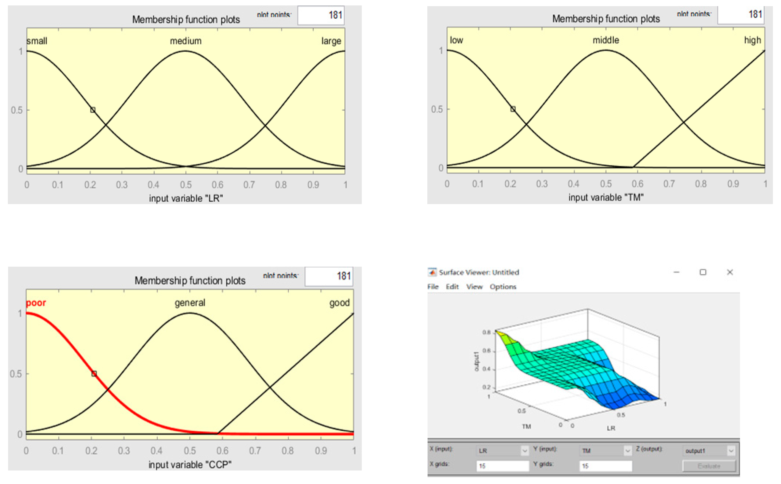
4.1.1. Fuzzy Variables

The entire system only makes basic disclosures—such as speed, direction, and location—while RSU and MEC servers make task queue disclosures to safeguard user privacy. The SNFLC algorithm aims to select a reliable server node RSU by integrating three performance indicators. In order to eliminate dimensional influence, the three indicators are normalized according to Equation (15) (that is, the domain of the three parameters are all (0, 1)), which can be used as the input of the algorithm [21].

$$Normal(var)=\frac{Value(var)-min(var)}{max(var)-min(var)}(var\in \{LR,TM,CCP\})$$

(15)

where, $Value(var)$ represents the actual variable performance value of a service node, $max(var),min(var)$ are, respectively, the maximum and minimum allowed theoretically for this performance, and the three normalized performance indexes are denoted as $\overline{LR},\overline{TM},\overline{CCP}$.

There are three types of commonly used fuzzy membership functions: triangular function, trapezoidal function and Gaussian function. The membership degree of triangular fuzzy function increases first and then decreases. It is suitable for describing well-defined nearby units. Where the definition is clear, the membership degree is the largest, but it allows a point to have the largest membership degree. The trapezoidal function is first raised and maintained for a period of time before decreasing, and its maximum membership can maintain its characteristic of maintaining a period to fit more real scenes. At the same time, when the maximum membership remains short enough, it is equal to triangular blur. Gaussian blur is the result of weighted average, which is more objective in theory. A Gaussian function is used to describe the membership degree of each fuzzy variable.

$$G(var)=\frac{1}{{\mathrm{e}}^{\frac{{[Normal(var)-\alpha ]}^2}{2{\beta }^2}}}$$

(16)

$\alpha ,\beta$ are an adjustable parameters used to correct the shape and offset point of the membership function. Meanwhile, in order to convert the normalized clear input features into fuzzy language variables, this study uses three fuzzy membership functions to fuzzify the clarity value of each feature. LR = {small, medium, large}, TM = {low, middle, high}, and CCP = {poor, general, good}, as shown in Figure 4.

4.1.2. Fuzzy Rules

The fuzzy set is composed of overlapping parts of each language variable [22]. In contrast, each language variable’s clear value is a member of the fuzzy set of each language variable, with varying degrees of participation. An IF-THEN rule is developed to represent the nature of this relationship and the various impacts of each parameter on node performance:

$$\mathrm{Rules} \mathrm{n}: \mathrm{IF} \overline{LR}(\tau ) \mathrm{is} A_{1n} \mathrm{and} \overline{TM}(\tau ) \mathrm{is} A_{2n} \mathrm{and} \overline{CCP}(\tau ) \mathrm{is} A_{3n}$$

$$\mathrm{THEN} F(\tau )=R_n(\tau )={\chi }_{0n}(\tau )+{\chi }_{1n}(\tau )*A_{1n}+{\chi }_{2n}(\tau )*A_{2n}+{\chi }_{3n}(\tau )*A_{3n}$$

where $A_{1n},A_{2\mathrm{n}},A_{3\mathrm{n}}$ are the corresponding language variable values of the three variables in the Nth rule; $R(\tau )$ is the fuzzy output value of this rule, and its mathematical relationship can be described as a linear polynomial function of three performance parameters. ${\chi }_{0n}(\tau )$ is a constant term with value 1, representing the coefficient of each parameter, so as to determine the relative influence degree of each feature and meet the following relationship [23]:

$${\displaystyle \sum _{\diamond =1}^3{\chi }_{\diamond n}(\tau )}=1, 0.0001\le {\chi }_{\diamond n}(\tau )<1$$

(17)

To ensure the minimum fairness, any item parameter cannot be zero, that is, every characteristic plays a part in assessing node performance. Theoretically, the fuzzy system has 3 inputs, and each input variable has 3 language values, and, at most, a $3^3$ rule can be established, as shown in

Table 1. Fuzzy rule table.

RULE	IF			THEN
	$\overline{\mathit{L}\mathit{R}}(\mathit{\tau })$	$\overline{\mathit{T}\mathit{M}}(\mathit{\tau })$	$\overline{\mathit{C}\mathit{C}\mathit{P}}(\mathit{\tau })$
1	small	low	none	$R_1(\tau )$
2	small	middle	none	$R_2(\tau )$
…	…	…	…	…
$3^3$	large	high	good	$R_{3^3}(\tau )$

.

The coefficients in the linear equation describing the outcome of the rules are further determined by the fact that not all rules are reasonable. The trial-and-error method is not the best option in this work because of the large number of tasks and poor efficiency involved, while the empirical method has too many subjective factors, making it impossible to ensure the validity of the results. Therefore, the gradient descent method is used to obtain the objective and reasonable coefficients by adjusting the coefficients of the above linear polynomial functions. Its performance indicator function is defined as follows:

$$\Theta (\tau )=\frac{{(\overline{LR}(\tau )-1)}^2+{(\overline{TM}(\tau )-1)}^2+{(\overline{CCP}(\tau )-1)}^2}{2}$$

(18)

In order to improve the stability of the algorithm, a set of forward coefficients $\{{\epsilon }_1,{\epsilon }_2,{\epsilon }_3\}({\epsilon }_1,{\epsilon }_2,{\epsilon }_3\in [0,1])$ that meet Lyapunov criterion are adopted, and the above functions are adjusted accordingly to obtain the modified coefficients, as shown in the following equations:

$$\begin{array}{ll}{\chi }_{1n}(\tau +1)& ={\chi }_{1n}(\tau )-{\epsilon }_1\frac{\partial \Theta (\tau )}{\partial {\chi }_{1n}(\tau )}\\ & ={\chi }_{1n}(\tau )-{\epsilon }_1\times (\overline{LR}(\tau )-1)\times {\chi }_{1n}(\tau )\times {\left[\frac{G^{\tau }(LR)-\Theta (\tau )}{{\chi }_{2n}^2(\tau )+{\chi }_{3n}^2(\tau )}\right]}^2\times {\gamma }_n(\tau )\end{array}$$

(19)

$$\begin{array}{ll}{\chi }_{2n}(\tau +1)& ={\chi }_{2n}(\tau )-{\epsilon }_2\frac{\partial \Theta (\tau )}{\partial {\chi }_{2n}(\tau )}\\ & ={\chi }_{2n}(\tau )-{\epsilon }_2\times (\overline{TM}(\tau )-1)\times {\chi }_{2n}(\tau )\times {\left[\frac{G^{\tau }(LR)-\Theta (\tau )}{{\chi }_{1n}^2(\tau )+{\chi }_{3n}^2(\tau )}\right]}^2\times {\gamma }_n(\tau )\end{array}$$

(20)

$$\begin{array}{ll}{\chi }_{3n}(\tau +1)& ={\chi }_{3n}(\tau )-{\epsilon }_1\frac{\partial \Theta (\tau )}{\partial {\chi }_{3n}(\tau )}\\ & ={\chi }_{3n}(\tau )-{\epsilon }_3\times (\overline{CCP}(\tau )-1)\times {\chi }_{3n}(\tau )\times {\left[\frac{G^{\tau }(LR)-\Theta (\tau )}{{\chi }_{1n}^2(\tau )+{\chi }_{2n}^2(\tau )}\right]}^2\times {\gamma }_n(\tau )\end{array}$$

(21)

where, ${\gamma }_n(\tau )$ is called the fuzzy basis function, and the specific expression is given in the following section. As seen from the diagram above, the system can identify a collection of appropriate dynamic adjustment performance coefficients $\{{\epsilon }_1,{\epsilon }_2,{\epsilon }_3\}$.

Set up the Lyapunov function:

$$E_{\Theta (\tau )}=\frac{1}{2}(E_{\overline{LR}(\tau )}^2+E_{\overline{TM}(\tau )}^2+E_{\overline{CCP}(\tau )}^2)$$

(22)

Introduce error variables:

$$\begin{array}{ll}err& =E_{\Theta (\tau +1)}-E_{\Theta (\tau )}\\ & =\frac{1}{2}{\displaystyle \sum _{\nabla }^{\overline{LR},\overline{TM},\overline{CCP}}(E_{\nabla (\tau +1)}^2-E_{\nabla (\tau )}^2)}\\ & =\frac{1}{2}{\displaystyle \sum _{\nabla }^{\overline{LR},\overline{TM},\overline{CCP}}(E_{\nabla (\tau +1)}^2+er{r}_{\nabla (\tau )}^2-E_{\nabla (\tau )}^2)}\end{array}$$

(23)

$$er{r}_{\overline{LR}(\tau )}^2=\frac{\partial E_{\overline{LR}(\tau )}}{\partial {\chi }_{1n}(\tau )}\cdot \Delta {\chi }_{1n}(\tau )=\frac{\partial E_{\overline{LR}(\tau )}}{\partial {\chi }_{1n}(\tau )}\cdot (-{\epsilon }_1\cdot E_{\overline{LR}(\tau )}\cdot \frac{\partial E_{\overline{LR}(\tau )}}{\partial {\chi }_{1n}(\tau )})$$

It can be concluded $er{r}_{\overline{TM}(\tau )}^2,er{r}_{\overline{CCP}(\tau )}^2$, from the above equation $err=\frac{1}{2}{\displaystyle \sum _{\nabla }^{\overline{LR},\overline{TM},\overline{CCP}}{\displaystyle \sum _{\diamond =1}^3{\displaystyle \sum _{\epsilon =1}^3(E_{\nabla (\tau )}\cdot \frac{\partial E_{\nabla (\tau )}}{\partial {\chi }_{\diamond n}(\tau )}{)}^2(\frac{\partial E_{\nabla (\tau )}}{\partial {\chi }_{\diamond n}(\tau )}}}}\cdot {\epsilon }^2-2\epsilon )$ that the convergence of the algorithm can be guaranteed only when $err<0$. Therefore, the value interval of the forward coefficient of the Lyapunov criterion is as follows:

$$0<\epsilon <{\epsilon }^{\prime },{\epsilon }^{\prime }=\left\{\begin{array}{l}1,{(\frac{\partial E_{\nabla (\tau )}}{\partial {\chi }_{\diamond n}(\tau )})}^2>\frac{1}{2}\\ {(\frac{\partial E_{\nabla (\tau )}}{\partial {\chi }_{\diamond n}(\tau )})}^2,{(\frac{\partial E_{\nabla (\tau )}}{\partial {\chi }_{\diamond n}(\tau )})}^2\le \frac{1}{2}\end{array}\right.$$

(24)

4.1.3. Solution of Fuzzy

The output results obtained by the fuzzy inference system are still fuzzy values. Defuzzing is required to transform them into readable and obvious values. According to the above fuzzy rules, the weighted average method is adopted, and the evaluation value of any RSU for the vehicle of the time slot $\tau$ is:

$${\psi }_i^j(\tau )=\frac{{\displaystyle \sum _{n=1}^{9}G(var)}{R}_n(\tau )}{{\displaystyle \sum _{n=1}^9{R}_n(\tau )}}={\displaystyle \sum _{n=1}^{9}G(var)}{\gamma }_n(\tau )$$

(25)

For each user vehicle, the result vector $[{\psi }_i^1(\tau ),{\psi }_i^2(\tau ),\dots ,{\psi }_i^j(\tau )]$ is finally generated as ${\psi }_i^j(\tau )$, to represent the performance evaluation value of the node j by user i through evaluating the nearby service nodes. The best service node is the maximum value $max({\psi }_i^j(\tau ))$ in vector. For the system, the final output is a vector $[V_1^j,V_2^j,\dots ,V_N^j](\tau )$ is made up of the best service nodes of all vehicles. The Algorithm 1 is shown as follows:

Algorithm 1: Service Node Selection Algorithm Based on Fuzzy Logic (SNFLC)

1: Enter vehicle information and RSU information 2: Output: vehicle optimal service node vector $[V_1^j,V_2^j,\dots ,V_N^j](\tau )$ 3: Initialize $t$= 0, and the number of vehicles 4: Each cycle $\Delta$ 5: $\Delta +\tau \to t$ 6: The service node releases information to all vehicles, and the vehicles broadcast requests to the system 7: for $v_i\in v_N \mathrm{do}:$ 8: The vehicle evaluates the performance of each service node according to the system information (LR, TM, CCP). 9: Use fuzzy inference system to output the evaluation result vector $[{\psi }_i^1(\tau ),{\psi }_i^2(\tau ),\dots ,{\psi }_i^j(\tau )]$ 10: Select the maximum value of the element in the vector $max({\psi }_i^j(\tau ))$ 11: End 12: Output the best service node vector $[V_1^j,V_2^j,\dots ,V_N^j](\tau ),V_N^j=max({\psi }_i^j(\tau ))$

4.2. Uninstallation Ratio and Resource Allocation

The analysis of optimization objective function P1 shows that constraint (8) is an integer variable, and other constraints are non-convex, so problem P1 is an NP problem that is difficult to solve directly [24]. Firstly, the problem is simplified. The integer constraint in the optimization objective is the key to the complexity of the problem. Here, it is relaxed into a continuous variable [25], that is, the discrete variable $\eta =\{0,1\}$ is transformed into a continuous variable $0\le \eta \le 1$. The restriction on task queue backlog can be disregarded here since it was considered in the prior service node selection [25]. Constraint (1) can be equivalent to $\left\{\begin{array}{l}{T}_{vi}^{local}\le T_{vi}^{max}\\ T_{vi,j}^{un}+T_{vi,j}^{wait}(\tau )+T_{vi,j}^{cal}\le T_{vi}^{max}\end{array}\right.$. Combining the above expressions, Equations (19) and (20) can be obtained as follows:

$$\begin{array}{ll}{T}_{vi}^{local}& =\frac{(1-\eta )S_{vi}^{local}}{Cycl{e}_{vi}}\\ & =\frac{(1-\eta )(1-a_{vi}^{\tau })S_{vi}}{\sqrt{\frac{{\Gamma }_{vi}^{local}}{\Phi (1-\eta )(1-a_{vi}^{\tau })S_{vi}}}}\\ & ={(1-a_{vi}^{\tau })}^{\frac{3}{2}}\sqrt{\frac{\Phi S_{vi}}{{\Gamma }_{vi}^{local}}}\le T_{vi}^{max}\end{array}$$

(26)

$$\begin{array}{l}{T}_{vi,j}^{un}+T_{vi,j}^{wait}(\tau )+T_{vi,j}^{cal}\\ =\frac{\eta S_{vi}^{un}}{r_{vi,j}^{un}(\tau )}+\frac{Q_j(\tau )-Q_j(\tau -1)}{{\Gamma }_{mec}}+\frac{S_{vi}^{un}}{f_{vi}^{mec}}\\ =\frac{a_{vi}^{\tau }{S}_{vi}}{B_{vi}{\log }_2(1+\frac{p_{vi,j}^{un}{\mathrm{H}}_{vi,j}}{{\mathrm{O}}^2})}+\frac{Q_j(\tau )-Q_j(\tau -1)}{{\Gamma }_{mec}}+\frac{a_{vi}^{\tau }{S}_{vi}}{{\Gamma }_{mec}}\le T_{vi}^{max}\\ =\frac{1}{B_{vi}{\log }_2(1+\frac{p_{vi,j}^{un}{\mathrm{H}}_{vi,j}}{{\mathrm{O}}^2})}\le \frac{T_{vi}^{max}}{a_{vi}^{\tau }{S}_{vi}}-\frac{Q_j(\tau )-Q_j(\tau -1)+1}{{\Gamma }_{mec}}\end{array}$$

(27)

By relaxing Equation (19) and substituting it into Equation (28), we obtain:

$$\frac{1}{B_{vi}}\le \left(\frac{{(1-a_{vi}^{\tau })}^{\frac{3}{2}}\sqrt{\frac{\Phi S_{vi}}{{\Gamma }_{vi}^{local}}} }{a_{vi}^{\tau }{S}_{vi}}-\frac{Q_j(\tau )-Q_j(\tau -1)+1}{{\Gamma }_{mec}}\right){\log }_2(1+\frac{p_{vi,j}^{un}{\mathrm{H}}_{vi,j}}{{\mathrm{O}}^2})$$

(28)

It can be seen from (18) that bandwidth resource is a variable related to unloading proportion, so the constraint on time of constraint (1) in problem P1 can be integrated into the bandwidth resource constraint, and the expression ${\overline{B}}_{vi}=\eta B_{vi},{\overline{P}}_{vi}^{mec}=\eta P_{vi}^{mec}$ of bandwidth and power resource is restated at the same time. The final problem P1 is restated as P2.

$$\begin{array}{l}\mathrm{P}2 \underset{\{a_{vi}^{\tau },P_{vi},B_{vi}\}}{min} e\\ s.t\\ {\displaystyle \sum _{vi=1}^N{\overline{B}}_{vi}\le B_{max}}\\ {\displaystyle \sum _{vi=1}^{vN}{\overline{P}}_{vi}}\le P_{max}\\ 0<a_{vi}^{\tau }<1\end{array}$$

(29)

The two variables are first decoupled in the revised problem P2 because the objective function and constraint conditions cause the bandwidth resources and unloading ratio to be mutually coupled. LC-IRA is proposed. For example, Algorithm 2 decomposed problem P2 into two sub-problems to reach an alternate optimization solution: (1) Given $a_{vi}^{\tau }$, solved resource allocation strategy (bandwidth and power) based on alternating direction multiplier method (ADMM); (2) Given $P_{vi},B_{vi}$, solve the unloading ratio $a_{vi}^{\tau }$. Problem P2.1 can be defined as:

$$\begin{array}{l}\mathrm{P}2.1 \underset{\{P_{vi},B_{vi}\}}{min} e\\ s.t\end{array}$$

(30)

The s.t constraint is equivalent to P2. Considering the independence between bandwidth resource allocation and power resource allocation, the following assumptions are proposed:

Assumption 1: Under the given unloading ratio, there exists an optimal solution $B_{vi}^{*},P_{vi}^{*}$ in problem P2.1, which meets Equation (31).

$$\left\{\begin{array}{l}{B}_{vi}^{*}=min(\frac{p_{vi,j}^{un}}{(\frac{p_{vi}^{local}}{a_{vi}^{\tau }Cycl{e}_{vi}}+\frac{1}{{\Gamma }_{mec}}-\frac{p_{vi}^{local}}{Cycl{e}_{vi}}){\log }_2(1+\frac{p_{vi,j}^{un}{\mathrm{H}}_{vi,j}}{{\mathrm{O}}^2}) },B_{max})\\ P_{vi}^{*}=min({\Gamma }_{mec}(\frac{p_{vi,j}^{un}}{{\log }_2(1+\frac{p_{vi,j}^{un}{\mathrm{H}}_{vi,j}}{{\mathrm{O}}^2})}+\frac{a_{vi}^{\tau }{p}_{vi}^{local}-p_{vi}^{local}}{a_{vi}^{\tau }Cycl{e}_{vi}}),P_{max})\end{array}\right.$$

(31)

Evidence: When the offloading ratio $a_{vi}^{\tau }$ is known, the constraint on bandwidth allocation $B_{vi}$ is no longer coupled, and the calculation power allocation $P_{vi}$ is independent of the former. The following is an example of how broadband resources can be optimized:

$$\begin{array}{l}\underset{B_{vi}}{min} \frac{p_{vi}^{local}{S}_{vi}}{Cycl{e}_{vi}}+a_{vi}^{\tau }{S}_{vi}(\frac{p_{vi,j}^{un}}{B_{vi}{\log }_2(1+\frac{p_{vi,j}^{un}{\mathrm{H}}_{vi,j}}{{\mathrm{O}}^2})}+\frac{P_{vi}}{{\Gamma }_{mec}}-\frac{p_{vi}^{local}}{Cycl{e}_{vi}}) \\ s.t\end{array}$$

(32)

The s.t constraint is equivalent to P2. In this case, the objective function is convex with respect to $B_{vi}$, and the constraint $\mathrm{ct}.1$ is also linear. $B_{vi}^{*}$ can be solved based on the basic convex optimization algorithm. In the same way, $P_{vi}^{*}$ can be obtained, as shown in Equation (32) above.

Then, the augmented Lagrange function is established:

$$\begin{array}{ll}{ƛ}_{\mu }(P_{vi},B_{vi},{\lambda }_1,{\lambda }_2)& =e-[({\lambda }_1,P_{max}-{\displaystyle \sum _{vi=1}^{vN}{\overline{P}}_{vi}})+({\lambda }_2,B_{max}-{\displaystyle \sum _{vi=1}^N{\overline{B}}_{vi}}) ]\\ & +\frac{\mu }{2}\left[{‖P_{max}-{\displaystyle \sum _{vi=1}^{vN}{\overline{P}}_{vi}}‖}^2+{‖B_{max}-{\displaystyle \sum _{vi=1}^N{\overline{B}}_{vi}}‖}^2\right]\end{array}$$

(33)

where $\lambda =\{{\lambda }_1,{\lambda }_2\}$ is the Lagrange multiplier and $\mu$ is the penalty parameter greater than 0. By introducing the concept of inertia strategy, the iteration expression of each parameter is redefined as follows:

$${\hat{P}}_{vi}^{\tau }=P_{vi}^{\tau }+\delta (P_{vi}^{\tau }-{\hat{P}}_{vi}^{\tau -1}),i=1,2\dots ,N,\delta \in [0,1)$$

(34)

$${\hat{B}}_{vi}^{\tau }=B_{vi}^{\tau }+\delta (B_{vi}^{\tau }-{\hat{B}}_{vi}^{\tau -1}),i=1,2\dots ,N$$

(35)

$$P_{vi}^{\tau +1}=\arg \min \left\{{ƛ}_{\mu }(P_{[1,vi-1]}^{\tau +1},P_{vi}^{\tau },P_{[vi+1,vN]}^{\tau },B_{vi}^{\tau },{\lambda }_1^{\tau })+\frac{1}{2}{‖P_{vi}-{\hat{P}}_{vi}^{\tau }‖}^2\right\}$$

(36)

$$B_{vi}^{\tau +1}=\arg \min \left\{{ƛ}_{\mu }(P_{vi}^{\tau },B_{[1,vi-1]}^{\tau +1},B_{vi}^{\tau },B_{[vi+1,vN]}^{\tau },{\lambda }_2^{\tau })+\frac{1}{2}{‖B_{vi}-{\hat{B}}_{vi}^{\tau }‖}^2\right\}$$

(37)

$${\lambda }^{\tau +\frac{1}{2}}={ƛ}^{\tau }-{\xi }_1\mu (P_{max}-{\displaystyle \sum _{vi=1}^{vN}{P}_{vi}}+B_{max}-{\displaystyle \sum _{vi=1}^N{B}_{vi}})$$

(38)

$${\lambda }^{\tau +1}={ƛ}^{\tau +\frac{1}{2}}-{\xi }_2\mu (P_{max}-{\displaystyle \sum _{vi=1}^{vN}{P}_{vi}}+B_{max}-{\displaystyle \sum _{vi=1}^N{B}_{vi}})$$

(39)

${\hat{P}}_{vi}^{\tau }$ is the improved inertia step, which improves the calculation accuracy numerically. $\delta$ is the acceleration coefficient to improve the convergence speed of the algorithm, and $\xi =\{{\xi }_1,{\xi }_2\}$ represents the error. The smaller the error value, the higher the convergence accuracy of the algorithm.

Issue P2.2 can be described as the issue of offloading ratio:

$$\begin{array}{l}\mathrm{P}2.2 \underset{a_{vi}^{\tau }}{min} \frac{p_{vi}^{local}{S}_{vi}}{Cycl{e}_{vi}}+a_{vi}^{\tau }{S}_{vi}(\frac{p_{vi,j}^{un}}{B_{vi}{\log }_2(1+\frac{p_{vi,j}^{un}{\mathrm{H}}_{vi,j}}{{\mathrm{O}}^2})}+\frac{P_{vi}}{{\Gamma }_{mec}}-\frac{p_{vi}^{local}}{Cycl{e}_{vi}})\\ s.t\\ \left(\frac{1}{B_{vi}^{*}{\log }_2(1+\frac{p_{vi,j}^{un}{\mathrm{H}}_{vi,j}}{{\mathrm{O}}^2})}-\frac{Q_j(\tau )-Q_j(\tau -1)+1}{{\Gamma }_{mec}}\right)\sqrt{\frac{S_{vi}{\Gamma }_{vi}^{local}}{\Phi }}\le \frac{{(1-a_{vi}^{\tau })}^{\frac{3}{2}} }{a_{vi}^{\tau }}\end{array}$$

(40)

In this case, the optimization objective is a linear function of the offload ratio $a_{vi}^{\tau }$. However, the positive and negative coefficients of $a_{vi}^{\tau }$ are unknown, so this function can be described as a linear function, $y(a_{vi}^{\tau })=\pm G{a}_{vi}^{\tau }+\frac{p_{vi}^{local}{S}_{vi}}{Cycl{e}_{vi}}$, which can be solved by ordinary linear equation solving methods with constraints.

Algorithm 2: A Low-Complexity Alternate Iteration Resource Allocation Algorithm (LC-IRA)

1: Initialization: The service node selects the vector, $P_{vi},B_{vi},{\lambda }_1,{\lambda }_2,\delta ,\mu >0,\tau =0$, and sets the minimum error value of iteration number $index=0$, ${\xi }_{min}$ as the convergence target of the algorithm. 2: Repeat 3: Update $P_{vi}^{\tau +1}$, according to Equation (26). 4: Update $B_{vi}^{\tau +1}$, according to Equation (27). 5: Update ${\lambda }^{\tau +\frac{1}{2}}$, according to Equation (28). 6: Update ${\lambda }^{\tau +1}$, according to Formula (29). 7: Update ${\xi }_1^{\tau +\frac{1}{2}}\leftarrow (P_{max}-{\displaystyle \sum _{vi=1}^{vN}{P}_{vi}})+(B_{max}-{\displaystyle \sum _{vi=1}^N{B}_{vi}})$ 8: Update ${\xi }_2^{\tau +1}\leftarrow {\lambda }^{\tau +\frac{1}{2}}-{\lambda }^{\tau }$ 9: Update ${\xi }^{\tau +1}\leftarrow \sqrt{{‖{\xi }_1^{\tau +\frac{1}{2}}‖}^2+{‖{\xi }_2^{\tau +1}‖}^2}$. 10: To compare the ${\xi }^{\tau +1}\le {\xi }_{min}$ 11: $index\leftarrow index+1$ 12: Until the algorithm converges 13. Solve problem P2.2 by using the linear equation solution method to obtain the optimal unloading proportion $a_{vi}^{*}$ 14: Output $P_{vi}^{*},B_{vi}^{*},a_{vi}^{*}$

After a fuzzy model, the optimization goal, and concrete calculation processing, each vehicle’s service node output evaluation values define the assessment points of maximum value, which are the best edge service nodes. The vehicle chooses the discharge to the node on the task, and, by adjusting the proportion of unloading, reasonable resource allocation, in order to achieve the optimization target of reducing system energy consumption.

5. Simulation Experiment

5.1. Simulation Experiment Environment

In this paper, Matlab is used to verify the algorithm of unloading edge computing tasks, including modeling application scenarios, and supporting various work on vehicle edge workflow, including model accuracy calibration, testing, etc. This experiment is based on Matlab 2019a for the Windows10 operating system. The scenario is set to an urban road intersection, the area is $\mathrm{A}=1000 \mathrm{m}\times 1000 \mathrm{m}$, there are $J=4$ RSU, each of which connects to one MEC server, the computing capability of the server is set to ${\Gamma }_{mec}=8 \mathrm{GHz}$, and the maximum bandwidth and power resources of the server are set to $B_{max}=2.5/\mathrm{Mbit},P_{max}=5.8/\mathrm{kw}$. The vehicle has a certain computing capability ${\Gamma }_{vi}^{local}=3 \mathrm{GHz},\forall i\in N$, and the number of vehicle tasks and the maximum allowable delay are evenly distributed in [50, 820]/Kb and [10, 50]/s. Finally, the minimum error threshold ${\xi }_{min}=0.001$ is specified in order to confirm the algorithm’s convergence.

Several other benchmark schemes are presented in order to assess the effectiveness of the suggested algorithm more accurately.

(1)

Service node selection

HDBSACAN: In reference [14], an improved hierarchical clustering algorithm (HDBSACAN) is proposed. Considering four performance indexes, an evaluation expression for surrounding service vehicles is proposed in order to find suitable service vehicles for task vehicles and improve task unloading efficiency.

Random selection (RS): As the intersection is special, the same vehicle can be in the communication range of multiple RSUs at the same time, and the vehicle randomly selects one of them as the service node.

F-SNFLC: In the fuzzy logic selection algorithm proposed in this paper, a fixed value is set for the coefficient of the output linear equation of the logic rule $F(\tau )$.

(2)

Resource allocation strategy algorithm

Average distribution (AD): Bandwidth $B_{max}$ and power $P_{max}$ are equally distributed to each vehicle. Task uninstallation ratio $a_{vi}^{\tau }=0.5$.

Random unloading allocation (RUA): A random seed function $rand$ is introduced to calculate the optimization objective so that the unloading ratio and resource allocation are randomly generated.

Genetic ant colony algorithm (G-ACA): the literature [21] considers a delay and energy consumption research uninstall strategy, and the algorithm integrates the benefits of the two basic algorithms. The improved shortcoming of the single algorithm easily falls into a local optimal solution, but it is insufficient, and the researchers will only use the algorithm in the single objective optimization scenario. Its performance in multi-objective optimization scenario is unknown.

Nonorthogonal multiple access (NOMA): according to the literature [2], the federation server allocation and power allocation, along with computing the allocation of resources, time distribution, and channel allocation, can minimize the total delay of all tasks. However, the authors did not take into consideration the unloading ratio and whether there is a coupling relationship between the resource allocation, which could be directly related to the ideal and displayed as a single variable.

5.2. Analysis of Experimental Results

When designing the fuzzy inference system, the researchers adjusted the Gaussian $\alpha ,\beta$ and modified the shape of the membership functions. Finally, a different service node was selected in order to verify this deviation, and the vehicle average cost was set as the evaluation criterion. The vehicle average cost is defined as the energy consumption and delay of accumulative and average $\cos t=\frac{1}{N}{\displaystyle \sum _{i=1}^N(E_{vi}^{local}+E_{vi,j}^{un}+T_{vi}^{local}+T_{vi,j}^{un}+T_{vi,j}^{wait}})$. The node is not the best option if the vehicle pays a higher fee there. According to Figure 5, if there is a difference between the two parameters, the Gaussian function will exhibit large fluctuations. The membership function of a fuzzy system’s input variables can also produce larger deviations. As shown in Figure 5, there is a gap between the two parameters, and the Gaussian function will have large fluctuations. The membership function of the fuzzy system input variables can produce larger deviation and evaluate the performance of the node deviation, which is greater than $\alpha ,\beta =0.5$. The more reasonable the parameters are, the more closely a vehicle can be matched to a service node, which makes it easier to allocate resources for subsequent work.

Figure 6 illustrates the differences in the various service node selection algorithms, the vehicle, and the final decision to use the CCP for Unicom. In other words, regardless of the algorithm used to find the best service node for the vehicle, the node and the vehicle must be able to establish a connection for Unicom to continue, and the probability of this happening is relatively low. The average CCP of the system will decrease as the number of vehicles rises, per the results, but the SNFLC-based algorithm suggested in this article performs best overall among all algorithms, followed by HDBSACAN. When clustering vehicles, the algorithm assigns a cluster head to each cluster, and, after computing duties are finished, the cluster head manages all the vehicles in the cluster jointly. When there are few vehicles, the results of the two algorithms are essentially the same, but as the number of vehicles rises, the shortcomings of the latter algorithm gradually become more obvious. This is because it is ignored that each vehicle is dynamically changing and that the evaluation of node performance has its own value. F-SNFLC is the second. Because this algorithm primarily establishes a fixed value in the fuzzy linear output equation that cannot be adjusted adaptively to changes in the system environment, performance degrades over time as the number of vehicles increases. N is the quantity of the car in Figure 6.

The convergence of the suggested resource distribution algorithm is confirmed, as seen in Figure 7. The algorithm gradually converges at around 700 iterations, and the average energy consumption gradually stabilizes, which is essentially consistent with the system’s lowest energy consumption.

The performance of the suggested algorithm is then evaluated in terms of system energy usage in comparison to other algorithms. According to Figure 8, the system’s energy consumption rises as the number of vehicles grows. The system load is significant when there are more than 80 system cars. The performance of G-ACA is reduced in the situation of multi-objective and large computation, and is even worse than the performance of the algorithm NOMA. Due to its high computational complexity, the NOMA algorithm performs less well than the LC-IRA algorithm suggested in this article. The efficiency of G-ACA, NOMA, and LC-IRA algorithms increased by 26.5%, 31.37%, and 45.52% in comparison to RUA and AD algorithms, respectively.

Figure 9 illustrates how each algorithm performs in terms of edge resource usage as the number of vehicles increases. With the increase in the number of vehicles, the task demand increases, the edge resources are fully utilized, and the utilization rate is improved. Due to the randomness of task unloading and resource allocation, RUA cannot be guaranteed to provide satisfactory services for vehicles, resulting in a small willingness to unload vehicles, which leads to the lowest utilization rate of edge resources. G-ACA is overtaken by NOMA once there are more than 200 vehicles because when the algorithm is used in multi-objective optimization scenarios, especially when the number of users increases dramatically, the algorithm performance declines, and it is unable to provide high-quality services for vehicles. The overall performance of LC is better than that of RUA, but it is still unable to provide appropriate services for vehicles. In the future, when the number of vehicles approaches 300, all of the vehicles can still share acceptable bandwidth and computing resources.

6. Conclusions

In this paper, a complex scenario of connected vehicle intersections is presented, along with a multi-service, multi-user edge computing task offloading and resource allocation approach with the aim of minimizing energy usage. The gradient descent technique is used to solve the fuzzy output linear equation in order to objectively choose the edge service nodes. The target problem is modeled as a mixed integer, high-complexity problem. By introducing a slack variable to validate the coupling between the discharge ratio and bandwidth resources; decoupling the problem into two sub-problems; using the ADMM method to solve the problems; and computing the best distribution of the power resources, the simulation results demonstrate that the algorithm is significantly less complex than other approaches. Specific contributions are as follows:

(1) In the scenario of complex connected vehicles at intersections, the optimization objective of minimizing system energy consumption is established by carefully considering the matching between users and service nodes, the unloading ratio, the bandwidth, and the resource allocation for computing power.

(2) A fuzzy logic-based service node selection method (SNFLC) is proposed considering the issue of matching users and service nodes. The linear equation describing the node performance value is found through fuzzy reasoning by specifying three performance indices as input. The equation’s coefficients are solved using the gradient descent technique, and the Lyapunov criterion coefficient is added to increase the algorithm’s stability. Finally, each node’s user evaluation number is output. The best service node is determined by the point with the highest evaluation value, and the vehicle decides to unload the task to this node.

(3) As the target problem is an NP problem, the coupling relationship between offloading ratio and bandwidth resource allocation is verified by relaxing integer variables, and the problem is decoupled into two sub-problems. LC-IRA is proposed to realize the resource allocation for bandwidth resource and computational power.

In the future, the authors will generalize the multi-unit task flow model under delay and energy consumption constraints by considering the heterogeneity of multiple users and the computing capacity ceiling for each user.

References

- Lin, H.; Zeadally, S.; Chen, Z.H.; Labiod, H.; Wang, L.S. A survey on computation offloading modeling for edge computing. J. Netw. Comput. Appl. 2020, 169, 102781. [Google Scholar] [CrossRef]
- Feng, C.; Han, P.C.; Zhang, X.; Yang, B.W.; Liu, Y.J.; Guo, L. Computation offloading in mobile edge computing networks: A survey. J. Netw. Comput. Appl. 2022, 202, 103366. [Google Scholar] [CrossRef]
- Islam, A.; Debnath, A.; Ghose, M.; Chakraborty, S. A survey on task offloading in multi-access edge computing. J. Syst. Archit. 2021, 118, 102225. [Google Scholar] [CrossRef]
- Hejja, K.; Berri, S.; Labiod, H. Network slicing with load-balancing for task offloading in vehicular edge computing. Veh. Commun. 2022, 34, 100419. [Google Scholar] [CrossRef]
- Liu, B.W.; Xu, X.L.; Qi, L.Y.; Ni, Q.; Dou, W.C. Task scheduling with precedence and placement constraints for resource utilization improvement in multi-user MEC environment. J. Syst. Archit. 2021, 114, 101970. [Google Scholar] [CrossRef]
- Wan, Z.L.; Xu, D.; Xu, D.H.; Ahmad, I. Joint computation offloading and resource allocation for NOMA-based multi-access mobile edge computing systems. Comput. Netw. 2021, 196, 108256. [Google Scholar] [CrossRef]
- Xiao, Z.; Shu, J.M.; Jiang, H.B.; Min, G.Y.; Chen, H.Y.; Han, Z. Perception task offloading with collaborative computation for autonomous driving. IEEE J. Sel. Areas Commun. 2023, 41, 457–473. [Google Scholar] [CrossRef]
- Jiang, H.; Dai, X.; Xiao, Z.; Iyengar, A.K. Joint Task Offloading and Resource Allocation for Energy-Constrained Mobile Edge Computing. IEEE Trans. Mob. Comput. 2022. [Google Scholar] [CrossRef]
- Li, Q.; Lin, H.; Tan, X.; Du, S. H∞ Consensus for Multiagent-Based Supply Chain Systems Under Switching Topology and Uncertain Demands. IEEE Trans. Syst. Man Cybern. Syst. 2020, 50, 4905–4918. [Google Scholar] [CrossRef]
- Lv, Z.; Qiao, L.; Li, J.; Song, H. Deep-learning-enabled security issues in the internet of things. IEEE Internet Things J. 2020, 8, 9531–9538. [Google Scholar] [CrossRef]
- Chen, Y. Research on collaborative innovation of key common technologies in new energy vehicle industry based on digital twin technology. Energy Rep. 2022, 8, 15399–15407. [Google Scholar] [CrossRef]
- Liao, Y.Z.; Shou, L.Q.; Yu, Q.; Ai, Q.S.; Liu, Q. Joint offloading decision and resource allocation for mobile edge computing enabled networks. Comput. Commun. 2020, 154, 361–369. [Google Scholar] [CrossRef]
- Xue, J.B.; Hu, Q.C.; An, Y.N.; Wang, L. Joint task offloading and resource allocation in vehicle-assisted multi-access edge computing. Comput. Commun. 2021, 177, 77–85. [Google Scholar] [CrossRef]
- Ju, X.; Su, S.C.; Xu, C.J.; Wang, H.X. Computation offloading and tasks scheduling for the internet of vehicles in edge computing: A deep reinforcement learning-based pointer network approach. Comput. Netw. 2023, 223, 109572. [Google Scholar] [CrossRef]
- Li, X.W.; Zhao, L.; Yu, K.P.; Aloqaily, M.; Jararweh, Y. A cooperative resource allocation model for IoT applications in mobile edge computing. Comput. Commun. 2021, 173, 183–191. [Google Scholar] [CrossRef]
- Zhao, J.; Xu, X.; Zhu, W.P. Adaptive delay-constrained resource allocation in mobile edge computing for Internet of Things communications networks. Comput. Commun. 2020, 160, 607–613. [Google Scholar] [CrossRef]
- Feng, H.; Guo, S.T.; Zhu, A.Q.; Wang, Q.Y.; Liu, D.F. Energy-efficient user selection and resource allocation in mobile edge computing. Ad. Hoc. Netw. 2020, 107, 102202. [Google Scholar] [CrossRef]
- Sadatdiynov, K.; Cui, L.Z.; Zhang, L.; Huang, J.Z.; Salloum, S.; Mahmud, M.S. A review of optimization methods for computation offloading in edge computing networks. Digit. Commun. Netw. 2022. [Google Scholar] [CrossRef]
- Lin, J.; Huang, L.; Zhang, H.L.; Yang, X.Y.; Zhao, P. A novel lyapunov based dynamic resource allocation for UAVs-assisted edge computing. Comput. Netw. 2022, 205, 108710. [Google Scholar] [CrossRef]
- Wang, K.; Wang, X.F.; Liu, X. A high reliable computing offloading strategy using deep reinforcement learning for iovs in edge computing. J. Grid Comput. 2021, 19, 15. [Google Scholar] [CrossRef]
- Saeed, J.; Mohammad, S.; Reza, M.; Amin, N.; Persico, V.; Pescapè, A. FUPE: A security driven task scheduling approach for SDN-based IoT–Fog networks. J. Inf. Secur. Appl. 2021, 60, 102853. [Google Scholar]
- Hamzah, A.; Shurman, M.; Al-Jarrah, O.; Taqieddin, E. Energy-efficient fuzzy-logic-based clustering technique for hierarchical routing protocols in wireless sensor networks. Sensors 2019, 19, 561. [Google Scholar] [CrossRef] [PubMed] [Green Version]
- Esmaeili, H.; Hakami, V.; Bidgoli, B.M.; Shokouhifar, M. Application-specific clustering in wireless sensor networks using combined fuzzy firefly algorithm and random forest. Expert Syst. Appl. 2022, 210, 118365. [Google Scholar] [CrossRef]
- Li, B.; Liu, W.S.; Fei, J.S. Offloading strategy of edge Computing tasks for empty space network. J. Electron. Inf. Technol. 2022, 44, 3091–3098. [Google Scholar]
- Xu, F.; Qin, Z.S.; Ning, L.P.; Zhang, Z.Y. Research on computing offloading strategy based on genetic ant colony fusion algorithm. Simul. Model. Pract. Theory 2022, 118, 102523. [Google Scholar] [CrossRef]