Monocular Depth Estimation Using Res-UNet with an Attention Model

Abstract

Depth maps are single image metrics that carry the information of a scene in three-dimensional axes. Accurate depth maps can recreate the 3D structure of a scene, which helps in understanding the full geometry of the objects within the scene. Depth maps can be generated from a single image or multiple images. Single-image depth mapping is also known as monocular depth mapping. Depth maps are ill-posed problems that are complex and require extensive calibration. Therefore, recent methods use deep learning to develop depth maps. We propose a new method in monocular depth estimation to develop a high-quality depth map. Our approach is based on a convolutional neural network in which we used Res-UNet with a spatial attention model to develop depth maps. The addition of an attention mechanism increases the capability of feature extraction and enhances the boundaries features. It does not add any extra parameters to the network. With our proposed model, we demonstrate that a simple CNN model aided with an attention mechanism can create high-quality depth maps with a small iteration and training time. Our model performs very well compared to the existing state-of-the-art methods on the benchmark NYU-depth v2 dataset. Our model is flexible and can be applied to any depth mapping or multi-segmentation tasks.

1. Introduction

Depth maps are created for respective RGB images to achieve distance information about the scene. Depth maps store the information of the scene in three-dimensional axes, i.e., xyz coordinates where z represents the distance of the object from the camera axes. Over the past few decades, extensive work has been conducted in 3D photogrammetry and depth mapping. Depth mapping has numerous applications in autonomous cars, robot navigation, remote sensing, 3D mapping, and obstacle detection. Depth estimation has been widely studied in computer vision and machine learning. A typical example of a depth map with its respective RGB image can be seen in Figure 1.

Initially, depth sensing was tackled with stereovision and structure from motion systems. These methods use the concepts of triangulation and stereo correspondence to calculate the disparity and depth, as seen in Figure 2a. Developing depth maps with these approaches requires calibrated cameras, a proper baseline, and template matching. Such approaches are complex and require extensive post-processing, making them less effective [1].

Similarly, some researchers have developed depth maps with special time-of-flight sensors (TOF) such as LIDAR, RADAR, and SONAR to calculate the depth of a scene [2,3]. Such devices use distance information and flight time to create depth maps. These TOF devices have many limitations, such as the amount of calibration required, lower resolution, difficulty of transport, and being bulky in nature. Additionally, these sensors are not energy efficient, which has reduced their application. A typical example of a TOF sensor is shown in Figure 2b. Recently, new depth cameras have been adopted to create depth maps [4]. Microsoft Kinect and 3D lidars are new devices used to estimate depth cues. These devices are also employed in creating datasets for machine learning and deep learning methodologies. Figure 2c shows a Microsoft Kinect 3D lidar depth sensor.

Depth mapping is an ill-posed problem because it can be generated from many respective scenes. Therefore, recently, depth maps have been developed with deep-learning methods. Many researchers have tried to solve depth problems using deep convolutional neural networks [5,6,7]. Deep-learning techniques are adopted to create depth maps because they can solve scale invariance and distorted boundary problems. In deep learning, the depth-estimation task is divided into three domains. The learning can be supervised, semi-supervised, and unsupervised to train the model [8]. In general, supervised learning requires the whole available dataset during training [9]. The unsupervised learning methodology does not require labeled datasets; rather, the datasets are generated during or before the training. Generally, unsupervised depth-mapping datasets are generated with traditional stereovision systems [10,11]. Similarly, semi-supervised learning is a hybrid type of learning where models are trained with partially labeled and partially unlabeled datasets.

In recent years, depth-map estimation has been studied widely in deep learning. However, there exist some limitations. Some of the major limitations are discussed as follows.

• Most of the depth maps suffer from inaccurate boundaries and edges which leads the model to a high level of errors and losses during training.
• Sometimes, models create depth maps which have scale invariance problems.
• In semi-supervised and unsupervised learning, the model learns from a stereovision system which requires extensive calibration and post-processing.
• Certain models are very complex and require a considerable amount of memory and training time to develop depth maps.

In order to address such shortcomings, we propose a simple encoder–decoder network in this paper. Our method is based on supervised learning, where we used complete datasets to train the network. In order to enhance the color features and boundaries of the objects, we added a spatial attention model in our network. The objective of this study is to develop a deep neural network which can create depth maps with a better accuracy and smaller errors. The main contributions of this paper are as follows.

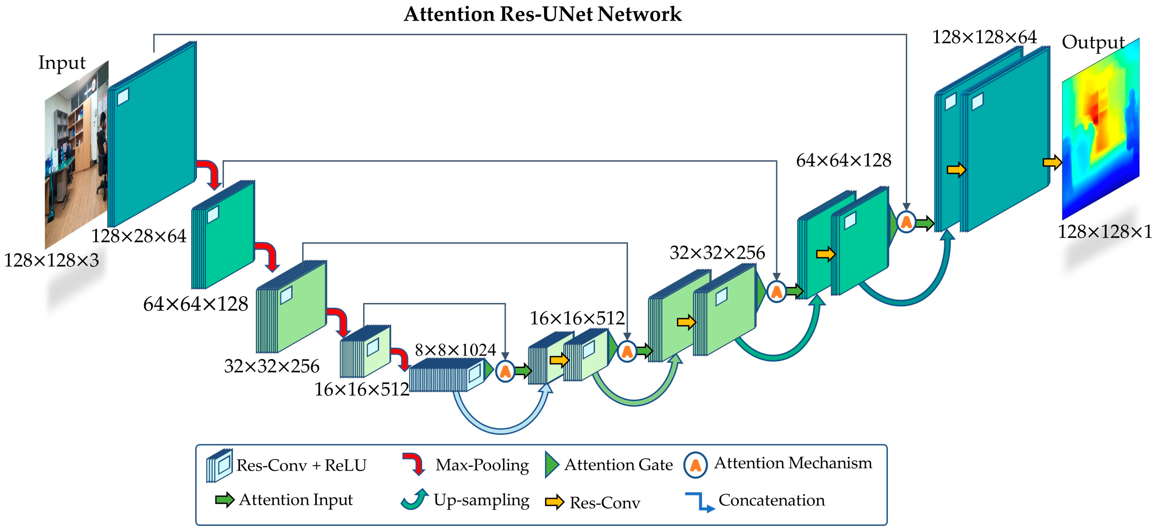
• We present a simple UNet architecture with Res-Net encoder–decoder blocks which can efficiently extract depth features from an input image.
• We added a spatial attention mechanism in our Res-UNet architecture which enhance the feature response and create clear boundaries and edges.
• We show that incorporating an attention mechanism did not increase the parameters in the model; rather, it helped the model to learn a greater number features in a shorter time with fewer iterations. The attention in the model suppresses the features response at the irrelevant locations while enhancing the response at relevant locations such as the edges or boundaries of depth maps.
• In summary, we created depth maps with a simple straight forward network which could be easily trained to any depth sensing or segmentation task.
• We trained our model on the publicly available NYU-depth v2 [4] and DIODE [12] datasets and achieved quality results.
• In conclusion, we discuss the findings, including the characterization of key parameters which influence performance, and outline avenues for future research in depth-mapping methodologies.

2. Related Work and Motivation

We grouped our literature review and related work into two main categories. We begin with an explanation of traditional depth-sensing techniques, and then we discuss state-of-the-art deep-learning methodologies.

2.1. Traditional Methods

Depth estimation is a very old concept in computer vision. It began with the theories of Wheatstone [13], who invented a stereoscope that proved that the brain uses horizontal disparity to find relative depth. Another researcher, Peddie et al. [14], discovered the depth from the structure of motion and proposed that objects at various distances move on the retinal surface at different speeds. This motion parallax allows the human brain to extract 3D shapes from motion. These theories were the foundation for multi-view depth mapping. For example, a depth map can be generated with the help of a stereovision system that uses template matching and horizontal disparity to calculate the depth. Similarly, a depth map can be created from the structure of motion where a single camera is moved with a constant baseline to develop a depth map [1].

Similarly, several researchers have tried to solve the depth problem from a single image. The possible work known in traditional methods is the work of Hoiem et al. [15]. They reconstructed a three-dimensional scene from a single RGB image for a virtual environment. Their approach was based on hand-crafted features, which categorized pixels into different classes based on their shapes and colors. Researchers such as Karsch et al. [16] and Ladický et al. [17] have used the theories of Hoeim et al. [15] to conduct depth analysis, calling it depth from semantic segmentation.

Ladický et al. [17] demonstrated the integration of monocular depth features with semantic object labels. They proposed a pixel-wise classifier that can jointly predict a semantic class and a depth label from a single image. Their model relied on manually created features and superpixels to segment the image. In their work, they require a proper alignment for semantic segmentation, which makes their runtime very slow. Karsch et al. [16] used a SIFT flow-based mechanism on KNN transfer to estimate static background depths from single images. In their model, they augmented motion information to estimate better moving foreground subjects in videos. This can result in better alignment and depth labels, but it necessitates having the entire dataset available at runtime and per-forming costly alignment procedures.

Saxena et al. [18] used synthetic data to estimate depth maps. Synthetic datasets consist of RGB images with their depth maps. Saxena et al. [18] applied custom-made filters to the input image in discrete sections. These filters calculated depth values for each small patch in a discrete section by processing the image information. Additionally, they used the Markov random field (MRF) model, which evaluated the absolute scales of several image patches and inferred the depth image.

Other researchers such as Karsch et al. [16] and Yang et al. [19] have used non-parametric methods to estimate the depth maps. In their work, the depth of a query image was calculated by fusing the depths of photos with related photometric content retrieved from a database. Depth images contain number of small features which are very useful in different applications. For rich feature extraction, a method of DFT can also be used; this method performs better in pattern recognition, artefact removal, and feature extraction [20].

When access to fast machines was limited, hand-crafted features were helpful. After years of progress, depth maps are tackled with high-speed computers and machine-learning techniques.

2.2. Depth Estimation Using Deep Learning

In order to develop depth maps, three types of learning methodologies are followed: supervised, semi-supervised, or unsupervised. When features are learned with all available datasets, this is known as supervised learning. Depth sensing in supervised learning is based on a single or monocular view. Datasets used in supervised learning are single RGB images with respective depth maps. Semi-supervised machine learning is a hybrid of supervised and unsupervised learning techniques. It employs a small amount of labeled data and a large amount of unlabeled data, providing the advantages of both unsupervised and supervised learning. Primarily, this technique relies on virtual data and certain auxiliary information. Similarly, in unsupervised learning, no ground truth dataset is used. The dataset fed in the network is prepared directly from epipolar geometry constraints. In certain cases, a stereo camera system is used to create a dataset before feeding it into the network [8]. Different types of learning techniques can be seen in Figure 3.

Our proposed method is based on supervised learning because it has many advantages. The significant advantage is that the model learns a greater number of features from the ground truth dataset, and they create very detailed depth maps. The model can be quickly evaluated, both qualitatively and quantitively, as the datasets provide test samples to elaborate the performance. We will briefly explain the methods by which depth maps are generated using different techniques.

2.2.1. Supervised Learning

Eigen et al. [5] were one of the first groups of researchers who attempted to use convolutional neural networks to predict a depth map from a single set of images. They used multi-scale deep neural networks to create depth maps for a respective RGB image. Their network had two stages: coarse level and fine level. The coarse-level network generated depths at a global level from the entire image. Later, the image from the coarse network, along with the original RGB image, was passed into the fine network. The fine network refined the predicted depth using local information. The network of Eigen et al. [5] was pre-trained on the ImageNet [21] classification task dataset. Using a pre-trained weight worked better because the network performs well if the training is initialized with some existing weights values rather than random initialization weights.

Eigen and Fergus [6] incorporated surface-normal and semantic labels to develop depth maps. They modified the model of Eigen et al. [5] by making their network deeper with more convolutional layers to estimate multi-channel feature maps. They used a single-scale, one-stack network. This combination resulted in combining depth and normal to share the computation load. Hence, they simultaneously predicted the depth and normal for a single RGB image. Their work shows that a VGG [22] based network performed better as compared to a small Alex-Net [21], but it failed to achieve sharp transitions.

In image processing, edges and lines are important features because they are used to detect object shapes in a scene. The deficiency in the above work of Eigen and Fergus [6] can be overcome by post-processing of the output results. A method of signal-to-noise ratio (SNR) proposed by Seo [23] can be applied to output depth maps to detect edges and lines. In his method, he analytically determined the SNR of the line and achieved quality results. We can enhance the output results by enhancing the lines and edges in the image. Similarly, for classification of each depth value, a method of wavelet transform can be performed on the predicted depth maps for smooth transitions during the post-processing [24,25,26].

Liu et al. [7] used conditional random fields (CRF) with CNNs to develop depth maps from single images. The use of convolutional neural fields helped to develop the connection between neighboring parts of depth maps. CRF nodes modeled a probability distribution function to optimize the neural network. Their network consists of two parts (unary and pairwise). The unary convolutional part aims to regress the depth values, and the pairwise potential part encourages neighbor super-pixels with the same appearance to take on the same depth values. The output from their network was a regressed depth for super-pixel values. The qualitative results of Liu et al. [7] have sharper transitions and aligned local structures. The drawback in their model was that scale invariance was not considered in their proposed work.

Laina et al. [27] proposed fully convolutional residual networks for depth estimation from a single image. They used a Res-Net 50 [28] encoder with pretrained weights in their model. Similarly, they proposed simple up-sampling and removed the last fully connected layers. This made their network simpler and more efficient. They used BerHu loss [29] during training, as this loss performed well compared to L2 loss when exploiting depth maps as ground truth. The outcomes of this study demonstrate that the value of applying up-projections in the decoder helps to produce dense output predictions with an improved resolution. Additionally, it demonstrates the possibility of employing Res-Net as the feature extractor rather than VGG or Alex-Net.

Similarly, Wang et al. [30] tried to use the global context CNN and regional CNN in a combined hierarchical conditional random field. They combined the work of Liu et al. [7] and Eigen et al. [5]. They used a global context CNN to estimate the semantic labels and depth in log space. The global context CNN was the same as in the model of Eigen et al. [5]. They only changed the last layer for semantic labels. Similarly, the regional CNN estimated the depth and semantic labels separately. The outputs from this network were semantic labels for segments and affinities to local depth templates. Such templates represent local structures such as corners, edges, and planes in a depth map. A shortcoming of this technique is that the algorithm could not estimate the absolute depth, as absolute depth cannot be estimated solely from local segments and predicted relative depth values. They solved this issue by deducting the absolute value of the pixel in the segment’s center and rescaling to the range <0, 1>.

Roy and Todorovic [31] proposed monocular depth estimation using a neural regression forest. They combined convolutional neural networks and a random regression forest with binary regression trees. Depth prediction for each pixel was estimated at the root tree node with the help of a convolutional window at the center of the image window. Their employed CNN contains pooling layers, which cause the resolution to decrease as the features go down the tree. This produces a multi-scale representation of the input. The fully connected layer at each node gives a probability of sending the output to the left or right child node. In order to ensure smooth depth predictions, the probability distribution predicted by the tree for pixel p is adjusted by bilateral filtering. Their quantitative results were better, but it fails in neural regression performance compared to previously dis-cussed methods.

In order to predict monocular depth, Fu et al. [32] developed a deep ordinal-regression network (DORN) using a multi-scale approach. They used a space-increasing discretization (SID) technique for depth data. Their depth-prediction mechanism was formulated as an ordinal regression problem, which aims to classify each pixel into a set of ordered categories while still possessing the characteristics of regression and classification. This approach considers that the uncertainty of depth prediction grows as depth values increase, enabling higher errors for deeper depth values. DORN uses atrous-spatial-pyramid-pooling with varying dilations and receptive fields of filters. Such spatial pyramid pooling prohibits the network from repeated convolution and pooling operations because repeated convolutions and pooling decrease the feature map sizes, which is undesirable for dense depth-prediction tasks. In their work, they compared VGG and Res-Net backbones and concluded that the Res-Net performance was the best.

Hu et al. [33] proposed two main improvements in depth-estimation tasks. Firstly, they used a multi-scale fusion module (MFM) to fuse extracted features at different scales with a refinement module. This module helped to combine discrete information at multiple scales into one. They used the same Res-Net proposed by Fu et al. [32] with a skip connection. Such lower-level information helped to recover a finer spatial resolution, which could be used to restore the minor detail lost due to multiple applications of downscaling. This resulted in clear boundaries in depth maps. Their second contribution was to develop a loss function that measures the inference error in training a model. They investigated the impact of various loss functions on the measurement of estimation errors near step edges. Their qualitative results show a better output of depth maps, but their network failed to accurately measure the reconstruction error of step edges for the evaluation of reconstruction accuracy.

Alhashim and Wonka [9] applied transfer learning to estimate the depth maps of a scene from a monocular image. They used a Dense-Net [34] encoder–decoder network with pretrained weights from ImageNet [21] to prevent training from random weights. The benefit of transfer learning helped to obtain greater feature extraction within a lower training time. They introduced a new loss function in which they combined different losses to estimate the depth maps. Their model was created on Dense-Net [34], which requires extensive memory. With a denser encoder, the number of parameters grows twice, which creates a serious caveat in training, making the learning slow. This represents the main drawback of their model. Another drawback is the overfitting due to color augmentation seen in their model.

Kumari et al. [35] generated depth images with the help of a residual encoder–decoder CNN network. Their model combined residual connections with hourglass networks that analyze the encoded characteristics at different scales. The inclusion of the hourglass module improved the output results, as this module emphasizes the export of global to local information by analyzing the different scales. Without the hourglass module, the results were suboptimal. They also added perceptual loss, which considered high-level features at different scales. The addition of perceptual loss helped the model to converge faster.

2.2.2. Semi-Supervised and Unsupervised Learning

Garg et al. [10] tried to solve the depth-estimation task in an unsupervised manner. They proposed a network and justified their work by comparing the weakness of supervised neural networks. They used an autoencoder setup to train on pairs of stereo images to construct depth maps. The encoder in their model was based on Alex-Net [21], in which the last connected layer is replaced with fully convolutional layers. Skip connections were introduced inside the network to obtain refined predictions. During training, the network predicts the inverse depth of the left image. Then, the right image, the disparity, and the predicted inverse depth of the left image are used by the network to reconstruct the left image. In the training phase, the reconstruction loss is reduced, and the reconstructed left image is matched to the input.

Godard et al. [11] also used unsupervised learning to estimated monocular depth. Their work was very similar to the method of Garg et al. [10]. The main difference in their method is that they introduced a new loss with left-right consistency. They showed that solely using reconstruction of the left image will lead to a poor depth prediction. Therefore, they used epipolar geometric constrains to generate disparity maps for both left and right images. They enforced the disparity maps’ consistency during the training phase, which improved the robustness and accuracy of the depth predictions. Their study demonstrated how a network could be trained in an unsupervised way for depth estimation using only stereo pairs of images.

Zhou et al. [36] created an unsupervised learning framework to simultaneously estimate the depth and ego-motion from a monocular camera. The training dataset was extracted from video recordings captured with a single camera. The camera location moves slightly between frames, behaving similar to a stereo pair. They developed a separate network to estimate the movement between the frames; hence, the camera calibration is eliminated. This method performed better, but certain assumptions were necessary for it to hold true. In order to prevent bad pixels from moving objects, which have a negative effect on the training process, they weighted the loss from each pixel using the predicted value for those pixels.

Following the trend, Casser et al. [37] proposed a motion model in an unsupervised approach. Their method can simulate dynamic scenes by simulating object motion. Their proposed motion model was the same as the ego-motion model. The only difference in their model was that it could precisely predict the motion of each individual object in 3D space. They used a pre-segmented RGB image sequence dataset for training. Hence, the model predicts the transformation vectors for each object in 3D space. Their method not only model the objects in 3D but also learns their motion on the fly. Their approach was able to model the depth for every scene and each individual object.

Chen et al. [38] estimated the depth from RGB images at a very sparse set of pixels. They used lower-power depth sensors to develop high-quality, dense depth maps. They combined semantic segmentation with sensor data to enhance the performance of the model. Their model was trained in a semi-supervised manner with a stereo camera setup. Their framework relies on both depth estimation and semantic segmentation, which switch according to conditions. Region-aware depth estimation is performed using a novel left –right semantic consistency term. They claim that their sparse depth information is very flexible, which leads the model to generalize the multiple scenes—meaning it can simultaneously work for indoor and outdoor scenes.

Mahjourian et al. [39] presented a new technique which uses the whole three-dimensional geometry of the scene, unlike previous depth-mapping methods which use the ego-motion, pixel-wise, or gradient-based losses in the small neighborhood. This technique considered the entire 3D scene and enforced the consistency of estimated 3D point clouds and ego-motion across all consecutive frames. They used a backpropagation algorithm for the alignment of 3D structures. Although their algorithm performed better than previously discussed work, it fails in a scenario where the object moves between two frames because their loss function misestimates the depth. In addition, their system needs to improve in largely dynamic scenes.

Finally, Goldman et al. [40] used a two-stream Siamese network [41] for monocular depth estimation. The Siamese neural network is trained on two networks simultaneously where one image is processed in one network and the other image is processed in another parallel network. The Siamese network learns to predict a disparity map from a single image. One of these networks is utilized during testing to determine the depth. Their network was able to be trained on a pair of stereo images simultaneously and symmetrically in a self-supervised way. Stereopair cameras were manually calibrated and placed at a proper baseline. Their network processed the input data in an unsupervised manner without labeling. No ground truth or labeled depth was provided to the network during training. The Siamese neural network [41] performed very well but the training time was doubled due to two-stream network behavior, as two networks were training on different images simultaneously. Similarly, the drawbacks of the traditional stereo camera system and post-processing were also the main drawbacks of their method.

3. Proposed Method

3.1. Overview

In this study, we build a fully convolutional Res-UNet with attention blocks for depth-map estimation. As a result of the effective use of GPU memory and outstanding speed, UNets are frequently employed for image-segmentation tasks. The latter benefit mostly involves extracting visual features at various image scales. As depth maps are similar to segmentation tasks, because depth values also behave as a multi-class classification task, we agreed on the idea of using Res-UNet with attention models in our model. In our proposed model, we replaced the simple two-dimensional convolutional layers with residual layers and we added attention models with spatial attention gates in the decoder layers. The schematic diagram is shown in Figure 4. We will explain our model in detail in all aspects below.

3.2. Proposed Model

UNets comprise an encoder–decoder model which is symmetric on both sides. The encoder uses a combination of convolutional layers and takes the spatial characteristics out of the original input image. From the extracted spatial features, the decoder creates depth maps. The decoder is made to up-sample and creates the necessary output masks or depth maps. In estimating depth maps, the model suffers from extracting boundaries and edges during training. Hence, we rebuilt the traditional UNet with residual blocks and added a spatial attention model at the decoder. Attention in a model mainly focuses on the small features, as well as edges and boundaries, to develop a very detailed depth map. The respective layers in our model are explained below.

3.2.1. Residual Network Block

In order to reduce the impact of network deterioration on model learning, He et al. [28] introduced Res-Net. In Res-Net, the accuracy deterioration, vanishing gradient, and large parameters problems were addressed. Such issues were resolved by the introduction of a skip connection with residual learning. Res-Net uses a shortcut to add the identity to each block’s output. It is different from traditional convolutional operations because it concatenates the features map directly into the decoding process. The input image latent representation is learned more effectively using the stacked residual block. The traditional 2D convolution block and residual block are shown in Figure 5.

In a deep residual learning framework, the residual convolution block aims to learn the output F(x), and identity (x), which results in F(x) + (x). Recasting the original mapping into F(x) + x, the network not only learns the features but also the residuals from the previous layers. The addition of identity assists the model to retain the features from the original input which helps in better feature learning. Additionally, the original map features (x) guide the model in backpropagation, which solves the problem of the vanishing gradient. The shortcut connection inside the residual block performs the identity mapping, and their resultant features are added to the outputs of stacked layers. This shortcut or skip connection never adds any extra parameters nor computational complexity. The entire network is fully connected and can be trained in an end-to-end manner with backpropagation. At output, the features are passed through a rectified linear unit (ReLU) activation function, and then to the proceeding layers. Mathematically, identity mapping and shortcuts can be represented as follows.

$$y=F\left(x, \left\{Wi\right\}\right)+x$$

(1)

Here, Equation (1) shows the building block of the residual layer. The $x$ and $y$ represent the input and the output vectors of the considered layer. The function $F\left(x, \left\{Wi\right\}\right)$ is the residual mapping, while x is an identity which is the same as input x. The operation on F(x) + x is element-wise addition. The x and F(x) must be of the same dimensions. If this is not the case, then linear projection can be performed by the shortcut connection to match the dimensions. Hence, the output will be as follows.

$$y=F\left(x,\left\{W_i\right\}\right)+W_{s}x$$

(2)

In Equation (2), the function $F\left(x,\left\{W_i\right\}\right)$ can represent multiple convolutional layers, whereas W_s represents the weights from the previous layer. The form of the residual function is very flexible, as more than two layers are possible within it [28]. The residual layer becomes a simple plain layer when only one layer exists inside the block, but this shows no advantage in feature extraction.

3.2.2. Attention Block

Attention in fully convolutional neural networks (CNNs) has been introduced for applications such as image captioning [42], machine translation [43], and classification [44]. Currently, attention gates are frequently employed in natural-image analysis, knowledge graphs, and language processing.

In CNNs, attention is implemented using one of two methods: post-hoc network analysis and trainable attention mechanisms. The former technique has mostly been used to gain access to network reasoning for the job of visual-object recognition [22,45]. Similarly, trainable attention is categorized as hard attention and soft attention. In our work, we adopted a soft trainable attention mechanism as it can be easily adopted in UNets.

(a)

Hard attention (Stochastic): Model training is more challenging in hard attention because of iterative region proposal and cropping [46]. These models are frequently non-differentiable and require reinforcement learning for parameter updates. Hard attention has been highly adopted in trainable transformers in recent times, as these models use iterative region proposal and cropping during feature learning.

(b)

Soft attention (Deterministic): Soft attention is probabilistic and uses normal backpropagation. These attention mechanisms do not require Monte Carlo or repeated random sampling. Soft attention is used to highlight the only relevant activation during training. It reduces the computational recourses wasted on irrelevant activations and provides a better generalization of the network. Additive soft attention has recently been used in image categorization and sentence-to-sentence translation [42,47].

Mathematically, soft attention can be written as follows.

$$E_{p\left(s_t|a\right)}\left[z_t\right]={\displaystyle \sum }_{i=1}^L{\alpha }_t{,}_{ i}{a}_i$$

(3)

Here, $E_{p\left(s_t|a\right)}$ denotes deterministic soft attention, $s_t$ is the attention location, $z_t$ is a context vector, $\alpha$ represents the weights, L corresponds to the features extracted at a different image location i.

The expectation of context vector $z_t$ is taken directly and deterministic attention is modeled by computing a soft attention weighted annotated vector ${{\displaystyle \sum }}_{i=1}^L{\alpha }_t{,}_i{a}_i$, as proposed by Bahdanau et al. [48]. This is equivalent to introducing a softly weighted context $\alpha$, into the system. The learning in attention is end-to-end with conventional backpropagation because the entire model is differentiable [49].

3.2.3. Attention Model in Depth Maps Estimation

In order to reduce the loss and improve the accuracy, current frameworks rely on additional preceding object localization models. We show that incorporating an attention mechanism into a common CNN model can accomplish the same goal. This does not necessitate the training of many additional model parameters or numerous models. The attention mechanism gradually reduces feature responses in irrelevant background regions [50]. This process does not need to crop the region of interest (ROI) between networks, in contrast to the localization strategy in multi-stage CNNs. The coefficients of attention, α ∈ [0, 1] in Equation (3), identify key image regions and prune feature responses to retain only the activations that are relevant to the task at hand. Input feature maps and attention coefficients are multiplied element-wise by attention gates to produce the output (see Equation (4)).

$$x_{i,c}^l=x_{i,c}^l·\alpha$$

(4)

Here, x^l is the feature map at the output of layer l, i and c denote the spatial and channel dimensions, and $\alpha$ is the attention weight coefficient. By default, each pixel vector $x_{i,c}^l\in R^{F_l}$ is given a single scalar attention value, where F_l is the number of feature-maps in the layer l. In our model we use multi-dimensional attention coefficients because there were several depth values (classes). We used additive attention to obtain gating coefficients following the same technique as Oktay et al. [50]. Despite requiring greater processing resources, this has been empirically proven to produce results that are more accurate than multiplicative attention. The formulation of additive attention is as follows.

$$q_{att}^l={\psi }^T\left({\sigma }_1\left(W_x^T{x}_i^l+W_g^T{g}_i+b_g\right)\right)+b_{\psi }$$

(5)

$${\alpha }_i^l={\sigma }_2\left(q_{att}^l\left(x_i^l, g_i;{\Phi }_{att}\right)\right)$$

(6)

Here, in Equations (5) and (6), ${\sigma }_2$ denotes the sigmoid activation function, $x_i^l$ and $g_i$ are features from the encoder and decoder layers. The attention gate is characterized by a set of parameters, ${\Phi }_{att}$, containing linear transformations: $W_x\in R^{F_{l}x{F}_{int}}$, $W_g\in R^{\left(F_{g}x{F}_{int}\right)}$, ${\psi }^T\in R^{\left(F_{intx1}\right)}$, and bias terms: $b_{\psi }\in R$, $b_g\in R^{\left(F_{int}\right)}$. $R^{\left(F_{int}\right)}$ represents dimensional intermediate space and $R^{\left(F_l\right)}$ is the dimensional feature-map layer. W_x represents the weights from the encoder layer, while W_g represents the weights generated from the gating signal from the decoder. ${\psi }^T$ is the linear transformation of the output. Here, the linear transform is performed by convolving a 1 × 1 × 1 channel-wise operation to the input tensor. Such an operation is termed vector concatenation-based attention. A sigmoid activation, ${\sigma }_2$, is used which results in better convergence for attention-gate parameters. The proposed attention mechanism is shown in Figure 6.

In Figure 6a, at the gating, there are two inputs g and x. The input g is coming from the decoder of the network, carrying better feature representation; x comes from the encoder through skip connections, meaning it has better spatial information. The job of attention is to pass those features which are more relevant to the output, such relevant features have higher weights while irrelevant features have lower weights. Attention is fed by both x and g at the same time. Attention applies a 1 × 1 convolution with a stride of 1 on input g, while on input x it applies a convolution of 1 × 1 with the stride of 2. The convolution with strides of 2 on x resizes its dimensions to the size of g. Thus, they are added with the same dimensions, and the operation can move forward to the next step.

In the next step, the attention decides whether the feature from the encoder or the feature from the decoder contains more information. The decision is performed by the ReLU activation function where aligned weights become larger while unaligned weights become relatively smaller. After the activation function, the features are passed through Ψ convolution which is a 1 × 1 operation with one filter. This operation reduces the number of filters to one. Here, the values are out of range because the ReLU activation function only passes the values that are greater than zero, such that:

$$\left(\right[max\left(0,ax\right)=a·max\left(0,x\right) for a>0\left]\right)$$

In order to bring values into the range of 0 and 1, we applied the sigmoid function. After the sigmoid function, the layers are resized to the original dimensions as input x. The outputs from this resampled layer are the weights from the sigmoid function. The size of the attention weights layer and input x are same, so they can be multiplied in an element-wise manner. Notably, the attention model only generates a weight matrix which is multiplied to input x for better features understanding. It does not create any extra parameters which increase the training time.

As an example, in Figure 6b at the final stage, each pixel value coming from x is multiplied by the weights coming from attention. The output has dimensions of 16 × 16 and, at the resampling phase in attention, the size of the weights matrix is also 16 × 16. Due to having the same dimensions, the attention weights can be multiplied to each layer of input x giving an output size of 16 × 16. This gives an element-wise updated output which can be inserted into the next layer. The weights are updated, as soft attention updates the weights in backpropagation. After all these operations, the output moves to the next layer and is concatenated with the next proceeding decoder.

3.2.4. Overall Architecture

Once the Res-Net block and attention block are created, they are incorporated into the UNet to perform the depth-map task. Initially, the residual layers are arranged in the encoder layers. Residual convolutional blocks are followed by 2D max-pooling layers. In our model, we use only four encoder layers similar to the original UNet [51]. The encoder is connected to the decoder by a bottleneck layer where the soft attention is incorporated. In the decoder, deconvolution or up-sampling is performed. The features are up-sampled by a factor of two. All of the layers are connected through skip connections with the addition of attention models. The summary of our proposed attention Res-UNet is shown in

Table 1. Summary of our proposed model.

Layer No.	Input Layer	Stride and Filters	Output
Encoder
Input	128 × 128 × 3	(1, 1, 64)	128 × 128 × 64
L1	128 × 128 × 64	(2, 2, 128) down-sampling	64 × 64 × 128
L2	64 × 64 × 128	(2, 2, 256) down-sampling	32 × 32 × 256
L3	32 × 32 × 256	(2, 2, 512) down-sampling	16 × 16 × 512
L4	16 × 16 × 512	(2, 2, 1024) down-sampling	8 × 8 × 1024
L5	Bottleneck (8 ×8 × 1024)
Decoder
att #1	Attention (L5, L4) (16× 16 × 512)		16 × 16 × 512
up #1	L5_up-sampling	(2, 2, 512)	16 × 16 × 512
L6	concatenation (att #1, up #1) + Res-Conv		16 × 16 × 512
att #2	Attention (L6, L3) (32 × 32 × 256)		32 × 32 × 256
up #2	L6_up-sampling	(2, 2, 256)	32 × 32 × 256
L7	concatenation (att #2, up #2) + Res-Conv		32 × 32 × 256
att #3	Attention (L7, L2) (64 × 64 × 128)		64 × 64 × 128
up #3	L7_up-sampling	(2, 2, 128)	64 × 64 × 128
L8	concatenation (att #3, up #3) + Res-Conv		64 × 64 × 128
att #4	Attention (L8, L1) (128 × 128 × 64)		128 × 128 × 64
up #4	L8_ re-sampling	(2, 2, 64)	128 × 128 × 64
L9	concatenation (att #4, up #4) + Res-Conv		128 × 128 × 64
Output	L9_re-sampling	(1, 1, 1)	128 × 128 × 1

.

3.2.5. Model Training

In the first step, the NYU-depth-v2 dataset was rearranged, and all the bad images were removed. The images along with depth maps were resized to 128 × 128 to input to the network. The size of input is not fixed and can be resized to any square size such as 128 × 128 and 256 × 256. In our case, we used a small input size due to memory limitations.

The images and depth maps were inputted into the first residual block. Inside a residual block, the images were convolved with a convolutional operation. Then, the output from the first conv-layer was passed through the second convolutional layer with batch normalization. After the second convolution, the output and the original input layers were added and passed through a ReLU activation function. This completed a whole residual block (Figure 7).

The output from the first residual block was passed through a 2D max-pooling layer which decreased its size. Our Res-UNet comprised four residual blocks, each followed by the max-pooling layer. Similar convolution and pooling were performed for proceeding layers until the bottleneck layer was reached. The bottleneck layer connected the encoder to the decoder. The decoder took the input from the last encoder layer concatenated with the attention model weights. The additive nature of attention made the model very slow, but it was capable of outstanding results. At the last decoder layer, the depth map was generated. The output from this layer was a single channel depth image.

3.2.6. Loss Function

For depth estimation, different types of loss function are used. The majority of methods use the mean squared error loss (MSE) and, in many cases, it performs very well. In our case, the model did not converge on MSE. We tried different types of loss functions, but none of them gave promising results. Hence, we borrowed the loss function from Alhashim and Wonka [9] and used it in our network. This loss function performed very well, and our model started to learn features and converged. During training, they defined the loss function L between the true label y and predicted y’ as the weighted sum of a three loss function.

Mathematically, the loss function is summarized as follows.

$$\left(y,y^{\prime }\right)=\lambda L_{depth}\left(y,y^{\prime }\right)+L_{grad}\left(y,y^{\prime }\right)+L_{ssim}\left(y,y^{\prime }\right)$$

(7)

The first term in Equation (7) is the $L_{1Pointwise}$ loss; similarly, the second term is the $L_{1Gradient}$ which is the loss over the image gradient; and the last term is the $L_{SSIM}$ which is the structural similarity term. Each of the above-mentioned losses are shown as follows.

$$L_{1Pointwise}=L_{depth}\left(y,y^{\prime }\right)=\frac{1}{n}{\displaystyle \sum }_p^n\left|y_p-y_p{}^{\prime }\right|$$

(8)

$$L_{1Gradient}=L_{grad}\left(y,y^{\prime }\right)=\frac{1}{n}{\displaystyle \sum }_p^n\left|g_x\left(y_p,y_p{}^{\prime }\right)\right|+\left|g_y\left(y_p,y_p{}^{\prime }\right)\right|$$

(9)

$$L_{SSIM}\left(y,y^{\prime }\right)=\frac{1-SSIM\left(y,y^{\prime }\right)}{2}$$

(10)

The term $\lambda$ in Equation (6) is the weight parameter for depth loss function. Empirically, the value was set to 0.1 as a reasonable weight for this term. Such loss terms have the inherent drawback of tending to grow as the ground-truth depth values increase. Researchers have considered the reciprocal of the depth to address this issue [52,53]. For the original depth map $y_{orig}$, they define the target depth map y as $y$ = $m/y_{orig}$ where m is the maximum depth in the scene. Other methods have considered transforming the depth values and computing the loss in the log space [5,53].

4. Results and Discussion

Depth mapping has been studied extensively in deep learning, and a variety of datasets are available for depth-sensing problems. A summary of different types of depth datasets is shown in

Table 2. Datasets used in deep learning for depth estimation.

Dataset	Type	Image Size
NYU-depth v2	Indoor and outdoor scenes	640 × 480
KITTI	Road environment	1280 × 384
Cityscapes	Urban streets	1024 × 2048
DIODE	Indoor and outdoor scenes	1024 × 768
Make3D	Outdoor scenes	1704 × 2272
Middlebury	Static indoor scenes	3000 × 2000

.

In this paper, we used two publicly available datasets to train our model. For comparative studies, we only used the NYU-depth v2 dataset, as the majority of state-of-the-art methods use this to test their network. We did not use the DIODE test data for results comparison studies. First, we will discuss the nature of the datasets used, then we will show qualitative and quantitative results. Then, we will compare our results with the state-of-the-art methods, and later we will briefly discuss our results.

4.1. Datasets

4.1.1. NYU-Depth v2

NYU-depth v2 [4] is composed of video sequences of 464 indoor scenes recorded with Microsoft Kinect. There are 120 k training samples and 654 testing samples. In our method, we used a subset of 50,000 images to train our algorithm. The upper bound of depth maps is 10 m. The original size of the image and its depth map in the dataset was 480 × 640, but we resized this to 128 × 128 due to GPU memory limitations. Our model was trained on a 128 × 128 size input which gives the same output size of 128 × 128. When testing, we computed the depth-map prediction of the entire test images, up-sampled it to 256 × 256, and then assessed it using the center cropping set out by Eigen et al. [5].

4.1.2. DIODE Dataset

The second dataset which we used in our training was the dense indoor and outdoor depth dataset (DIODE) [12]. DIODE is a dataset that contains diverse high-resolution color images with accurate, dense, far-range depth measurements. The dataset includes RGBD images of indoor and outdoor scenes obtained with one sensor suite. We only took the training dataset of indoor scenes which comprised 8574 images with test images of 753 images. The original size of input images with their respective depth values were 1024 × 786 but due to our memory limitation we reduced the size to 256 × 256 in training the model. At testing, we computed depth maps with the resolution of 256 × 256, the same as the input size to the model.

4.2. Evaluation Results

4.2.1. Quantitative Evaluation

Methods for monocular depth estimation have been evaluated using different metrices. We quantitatively compare our method against state-of-the-art methods using the six standard metrics. These error metrics are defined as:

1. 

Average relative error

$$Rel=\frac{1}{n}{\displaystyle \sum }_p^n\frac{\left|y_p-y_p{}^{\prime }\right|}{y_p}$$

(11)

2. 

Root mean square error

$$RMS=\sqrt{\frac{1}{n}{\displaystyle \sum }_p^n{\left(y_p-y_p{}^{\prime }\right)}^2}$$

(12)

3. 

Average error

$$Log10=\frac{1}{n}{\displaystyle \sum }_p^n\left|lo{g}_{10}\left(y_p\right)-lo{g}_{10}\left(y_p{}^{\prime }\right)\right|$$

(13)

4. 

Threshold accuracy

$$\left({\delta }_i\right)=\%\mathrm{of}{y}_p\mathrm{suchthat},max\left(\frac{y_p}{y_p{}^{\prime }},\frac{y_p{}^{\prime }}{y_p}\right)<{1.25}^i\left(i=1,2,3\right)$$

(14)

In above metrices, $y_p$ is the pixel in depth image $y$, $y_p{}^{\prime }$ is a pixel in predicted image, and $n$ is the total number of pixels for each depth image. The results of the NYU-depth v2 dataset compared with state-of-the-art methods are listed in

Table 3. Quantitative comparison of different state-of-the-art methods on the NYU-depth v2 dataset.

Methods	High Is Better ↑			Low Is Better ↓
	${\mathit{\delta }}_1$ ↑	${\mathit{\delta }}_2\uparrow$	${\mathit{\delta }}_3\uparrow$	Rel↓	RMS↓	Log10↓
Eigen et al. [5]	0.769	0.950	0.988	0.158	0.641	-
Laina et al. [27]	0.811	0.953	0.988	0.127	0.573	0.055
Fu et al. [32]	0.828	0.965	0.992	0.115	0.509	0.051
Alhashim and Wonka [9]	0.846	0.974	0.994	0.123	0.465	0.053
Ours (scaled)	0.917	0.987	0.993	0.117	0.398	0.047

.

4.2.2. Qualitative Results

Figure 8 shows the predicted depth maps of the networks trained on the NYU-depth v2 dataset using an Eigen split [5]. The images were chosen for the visual inspection because they highlight the different strengths and weaknesses of the networks. All images were taken from the test set to assess the networks’ ability to generalize to data they had never seen before. The results were also compared to different state-of-the-art methods. It can be seen in last column of the Figure 8 that our depth maps are clear with crisp boundaries.

The maximum predicted depth values vary between networks, and each prediction has its own color scale. The colors in depth maps represent the predicted depth in meters, with red corresponding to large depth values and blue corresponding to small depth values. Each figure depicts the input image, the corresponding depth ground truth, and the prediction of each network.

We also tested our model on our random indoor scene images, and it shows quality results, as can be seen in Figure 9.

4.3. Implementation Details

We implemented our proposed attention Res-UNet depth network using the Python programming language. The workstation setup is summarized in

Table 4. System information for model implementation.

Components		Title 3
Hardware	CPU GPU SSD	Intel(R) Core (TM) i5-11400F 8 GB GeForce RTX 3050 500 GB Samsung SSD
	RAM	16 GB
Software	OS Programming Platform Library	Windows 11 Pro, 64 bits Python 3.8 TensorFlow 2+

. The code was built and implemented using Python programming language with CUDA TensorFlow 2.2.0.

Our encoder was composed of four original Res-Net-blocks with no pretrained weights. All the network training was started from default random weights. In all experiments, we used the Adam optimizer [54] with a learning rate of 0.001 with default parameter values of alpha and beta. The batch sizes were set to 8 and 16. The total number of trainable parameters for the entire network was 32.6 M.

4.3.1. Learning Curve for the DIODE Dataset

We trained our model on the DIODE dataset with random weights; after 40 epochs, the loss started to reduce, showing the trend that the model is training in the right direction as shown in Figure 10.

During training, the learning rate was set to 0.001 with the Adam optimizer. Similarly, due to GPU occupancy, we set our batch size to 16 for the DIODE dataset. We can see that validation loss, as well as training loss, decreased with the number of epochs which means that the model is learning the features with minimal loss. During the training of the model, the input size of each image was 256 × 256. The DIODE dataset took 11 h to train the model.

4.3.2. Learning Curve for the NYU-Depth v2 Dataset

We trained the same model for 20 epochs on the NYU-depth v2 dataset with the input size of 128 × 128, because the dataset size was very large and it required more time to train. We set the batch size to 8 due to GPU memory. Similarly, the same Adam optimizer was used with the learning rate of 0.001. The model took approximately 26 h on the NYU-depth v2 dataset. We also experimented on the same dataset with the input size of 256 × 256 which took around 3 days to train, and the results were almost identical with those of the previous model. The training curve is shown in Figure 11.

4.4. Discussion

Throughout this study, we investigated new ways to simplify depth procedures and develop an algorithm that is straightforward and reliable with good visual and numerical results.

4.4.1. Depth-Estimation Algorithm

In this study, we presented a deep neural network architecture for monocular depth estimation. Our architecture contains four layers, with each layer as a residual block. Each residual block performed well in extracting depth information. On the decoder, we generated feature information with the help of a smart attention model. This gave us not only better qualitative results but also quantitative results. Certain test results from the NYU-depth v2 dataset are shown in Figure 12.

Our proposed network has approximately 39 million parameters and is a large and sophisticated network. As a result of having such parameters compared with the baseline, the model requires extensive computational and memory resources. The potential for real-time performance is further constrained by the network’s high degree of complexity. We trained our network on squared input images, but it is not limited to a fixed input size. If the GPU memory is sufficient, the network can accept any image with a size divisible by 16 and return the result.

It could also be easily modified to accept any sized image, although this would require some interpolation steps. Our model can also easily be adapted to the task of semantic segmentation or other pixel-wise dense prediction tasks. This property, together with the non-fixed input size, make it simple to retrain the network for new tasks with different datasets and input sizes.

4.4.2. Evaluation Analysis

The visual results, as well as the error metrics, were studied to evaluate the performance of the networks. The error metrics provide an objective assessment of the average performance across the entire test set, whereas the visual inspection, which was limited to a few images, cannot be considered to represent the distribution of the entire dataset. In order to obtain a more reliable qualitative evaluation, a larger number of predictions should be inspected and evaluated in a more structured manner by several people.

As a result, the quantitative results were regarded as more reliable, and a greater weight was placed on them when determining the best network architecture. The quantitative analysis, however, is not without flaws. Quantitative analysis compares the predicted results with ground truth. This means the error metrics only assess how effectively the network predicts the depth values in relation to the given ground truth.

4.5. Ablation Study

4.5.1. Hyperparameters and Training

Hyperparameters—such as dropout, learning rate, optimizers, and batch size—searches were conducted to a considerable extent. During experimentation, small tweaks in hyperparameters were performed to check the model performance. For example, we used a 10% rate of dropout during training to ascertain the training behavior which resulted in better model convergence. Increasing the dropout from 10% also reduced the performance of our network. Similarly, trial and error were used to determine the learning rate and batch size. During trials, we started from standard learning rates such as 0.01, 0.001, and 0.0001. After certain epochs, we found that a learning rate of 0.001 performs better than the other learning rates and the model started to learn the features with fewer errors. In addition to that, an ADAM optimizer was used during training, because Res-Net performed better with an ADAM optimizer as compared to an SGD optimizer. The weight decay and the alpha and beta values of the optimizer were used as the default. Only the baseline network was subjected to the hyperparameter search. The base network was taken as an experimental model for the best fit parameters search. Due to the complex nature of our model, we checked for small changes during the hyperparameter search but, even with small iterations, we achieved quality results. We developed a simple attention Res-UNet for depth estimation in which we used simple model hyperparameters. We tested several more hyperparameters within a close range of the optimum values, but the results did not improve further.

4.5.2. Loss Function

During training, we used different loss functions but the model did not converge. We used the depth loss function borrowed from Alhashim and Wonka [9] and it returned very good results. Our model was trained with minimum loss and, on limited epochs, we achieved promising results. Our loss function has four parameters. The parameters are lambda, depth loss, depth gradient loss, and depth structural similarity loss. The depth loss measures the difference between the predicted and original depth maps. Depth gradient loss measures the gradient magnitude between the predicted depth image and the ground truth depth image. This loss encourages the model to produce images with similar gradient magnitudes. Similarly, structure similarity loss measures the similarity between the true and predicted depth maps. SSIM loss helps the model to predict depth maps which are structurally similar to the ground truth. All of the parameters are dependent on each other. We checked different combinations of these parameters, where only the cumulative results of these losses started to train our model. A brief summary of the experimentation of such losses is shown in

Table 5. Effect of change in loss parameters on model training.

Loss Functions	Training Loss	Output
$\left(y,y^{\prime }\right)=0.1L_{depth}\left(y,y^{\prime }\right)+L_{grad}\left(y,y^{\prime }\right)+L_{ssim}\left(y,y^{\prime }\right)$	0.0094	Model was trained to minimum loss
$\left(y,y^{\prime }\right)=0.2L_{depth}\left(y,y^{\prime }\right)+L_{grad}\left(y,y^{\prime }\right)+L_{ssim}\left(y,y^{\prime }\right)$	0.0251	Model was trained to acceptable loss
$\left(y,y^{\prime }\right)=0.3L_{depth}\left(y,y^{\prime }\right)+L_{grad}\left(y,y^{\prime }\right)+L_{ssim}\left(y,y^{\prime }\right)$	0.0291	Model was trained to acceptable loss
$\left(y,y^{\prime }\right)=0.1L_{depth}\left(y,y^{\prime }\right)+L_{grad}\left(y,y^{\prime }\right)$	0.0261	Model failed at 4th epoch
$\left(y,y^{\prime }\right)=0.1L_{depth}\left(y,y^{\prime }\right)+L_{ssim}\left(y,y^{\prime }\right)$	0.0557	Model failed at 6th epoch
$\left(y,y^{\prime }\right)=L_{grad}\left(y,y^{\prime }\right)+L_{ssim}\left(y,y^{\prime }\right)$	0.0207	Model failed at 2nd epoch
$\left(y,y^{\prime }\right)=0.1L_{depth}\left(y,y^{\prime }\right)$	0.096	Model failed at 1st epoch

below.

From the Table 5 we can see that all the loss parameters are highly dependent on each other. Even if we change one value, the model will not train properly. Hence, we used the combination of all parameters in our training loss with a lambda of 0.1 to achieve the best performance. The effect of lambda can also be seen in Figure 13.

In depth maps, loss function plays a key role and proper attention should be given to it. Loss functions compares the actual or ground truth values to the predicted value. If the loss value is minimum, it means the model accurately created the depth map, and the model is learning in a right way. If the loss values are higher, it means the model did not detect the depth values correctly.

Sometimes the loss metric gives larger errors for larger depths. By larger depths, we mean that the model detects the far pixels incorrectly. Most of the time, this can be allowed for far objects, but for near objects with smaller depths if the error is more, it could be catastrophic. For example, in autonomous cars, if the depth is 70 m and the prediction is 65 m, this can be allowed, as the obstacle is far from a car; however, for near objects if the loss is more, this is not allowed because the car is already near to the obstacle. Therefore, the network loss metric should focus on the weights for smaller depths, such that the close predictions could be estimated more accurately.

5. Conclusions and Future Work

The primary goal of this study was to implement, train, and evaluate a neural network that predicts the depth map from monocular RGB images. Our network predicts the depth map from monocular images with an accuracy comparable to state-of-the-art methods. We applied residuals block with an attention model in a traditional UNet. Our work was inspired by current trends in learning-based depth estimation research, which emphasizes accuracy improvement at the expense of larger models and more sophisticated computations. Modern depth-estimation techniques frequently use deep neural networks, which need considerable processing power and are just too complex to operate on real world data.

Upon the completion of this study, we came up with some future work suggestions that focus on improving the network performance. In order to increase the network performance, more labeled datasets are required. Current depth datasets are very limited. New and more labeled datasets could help in training the networks more accurately. Additional data augmentations, such as spatial scaling, color, brightness, and contrast augmentations, could be used to provide more varied data to the network. This would train the network to better generalize to new scenes.

Similarly, we built this model on the idea of semantic segmentation, as depth maps are very similar to semantic segmentation tasks. The network could be modified to perform semantic segmentation and depth estimation simultaneously because both the semantic labels and the depths share context information. Thus, semantic labels could be used to guide and presumably improve depth prediction. In addition, this work has focused on both the encoder and decoder parts of the network. We agreed on the residual block, as this performed well on classification tasks and it reduced the problem of vanishing gradient. However, the choice of one type of backbone is not limited to such a network. Currently, new and more efficient encoders such as MobileNets, EfficientNets, and vision transformers are being developed which can achieve state-of-the-art results on ImageNet classification tasks. Such encoders are possible to incorporate inside the UNets, but further study is required to check their performance. We will look for a more efficient and denser encoder and decoder to train on depth-estimation tasks. The transformers are becoming the new standard in image processing tasks, as they are fast and lightweight. Current transformers are smart features extractors which have fewer parameters. In future studies, we may experiment with vision transformers to verify whether they can develop dense depth maps. Similarly, a variety of attention models can be incorporated into new networks. There is also a chance that the network will become so lightweight that it can perform depth-estimation tasks in real time.

References

1. Hartley, R.; Zisserman, A. Multiple View Geometry in Computer Vision, 2nd ed.; Cambridge University Press: Cambridge, UK, 2004; ISBN 978-0-521-54051-3. [Google Scholar]
2. Leonard, J.J.; Durrant-Whyte, H.F. Mobile Robot Localization by Tracking Geometric Beacons. IEEE Trans. Robot. Autom. 1991, 7, 376–382. [Google Scholar] [CrossRef]
3. Leonard, J.J.; Durrant-Whyte, H.F.; Pj, O. Directed Sonar Sensing for Mobile Robot Navigation; Springer Science & Business Media: Berlin/Heidelberg, Germany, 2002. [Google Scholar]
4. Silberman, N.; Hoiem, D.; Kohli, P.; Fergus, R. Indoor Segmentation and Support Inference from RGBD Images. In Computer Vision—ECCV 2012; Fitzgibbon, A., Lazebnik, S., Perona, P., Sato, Y., Schmid, C., Eds.; Lecture Notes in Computer Science; Springer: Berlin/Heidelberg, Germany, 2012; Volume 7576, pp. 746–760. ISBN 978-3-642-33714-7. [Google Scholar]
5. Eigen, D.; Puhrsch, C.; Fergus, R. Depth Map Prediction from a Single Image Using a Multi-Scale Deep Network. arXiv 2014, arXiv:1406.2283. [Google Scholar]
6. Eigen, D.; Fergus, R. Predicting Depth, Surface Normals and Semantic Labels with a Common Multi-Scale Convolutional Architecture. arXiv 2015, arXiv:1411.4734. [Google Scholar]
7. Liu, F.; Shen, C.; Lin, G.; Reid, I. Learning Depth from Single Monocular Images Using Deep Convolutional Neural Fields. IEEE Trans. Pattern Anal. Mach. Intell. 2016, 38, 2024–2039. [Google Scholar] [CrossRef] [PubMed]
8. Jan, A.; Khan, S.; Seo, S. Deep Learning-Based Depth Map Estimation: A Review. Korean J. Remote Sens. 2023, 39, 1–21. [Google Scholar]
9. Alhashim, I.; Wonka, P. High Quality Monocular Depth Estimation via Transfer Learning. arXiv 2018, arXiv:1812.11941. [Google Scholar]
10. Garg, R.; Bg, V.K.; Carneiro, G.; Reid, I. Unsupervised CNN for Single View Depth Estimation: Geometry to the Rescue. In Computer Vision–ECCV 2016: 14th European Conference, Amsterdam, The Netherlands, October 11–14, 2016, Proceedings, Part VIII 14 2016; Springer International Publishing: Berlin/Heidelberg, Germany, 2016; pp. 740–756. [Google Scholar]
11. Godard, C.; Mac Aodha, O.; Brostow, G.J. Unsupervised Monocular Depth Estimation with Left-Right Consistency. arXiv 2017, arXiv:1609.03677. [Google Scholar]
12. Vasiljevic, I.; Kolkin, N.; Zhang, S.; Luo, R.; Wang, H.; Dai, F.Z.; Daniele, A.F.; Mostajabi, M.; Basart, S.; Walter, M.R.; et al. DIODE: A Dense Indoor and Outdoor DEpth Dataset. arXiv 2019, arXiv:1908.00463. [Google Scholar]
13. Wheatstone, C. XVIII. Contributions to the Physiology of Vision—Part the First. On Some Remarkable, and Hitherto Unobserved, Phenomena of Binocular Vision. Phil. Trans. R. Soc. 1838, 128, 371–394. [Google Scholar] [CrossRef]
14. Peddie, W. Helmholtz’s Treatise on Physiological Optics. Nature 1925, 116, 88–89. [Google Scholar] [CrossRef]
15. Hoiem, D.; Efros, A.A.; Hebert, M. Automatic Photo Pop-up: ACM SIGGRAPH 2005. ACM Trans. Comput. Syst. 2005, 24, 577–584. [Google Scholar] [CrossRef]
16. Karsch, K.; Liu, C.; Kang, S.B. Depth Transfer: Depth Extraction from Video Using Non-Parametric Sampling. IEEE Trans. Pattern Anal. Mach. Intell. 2014, 36, 2144–2158. [Google Scholar] [CrossRef]
17. Ladický, L.; Shi, J.; Pollefeys, M. Pulling Things out of Perspective. In Proceedings of the 2014 IEEE Conference on Computer Vision and Pattern Recognition, Columbus, OH, USA, 23–28 June 2014; pp. 89–96. [Google Scholar]
18. Saxena, A.; Chung, S.; Ng, A. Learning Depth from Single Monocular Images. In Proceedings of the Advances in Neural Information Processing Systems, Vancouver, BC, Canada, 5–8 December 2005; MIT Press: Cambridge, MA, USA, 2005; Volume 18. [Google Scholar]
19. Yang, J.; Alvarez, J.M.; Liu, M. Non-Parametric Depth Distribution Modelling Based Depth Inference for Multi-View Stereo. In Proceedings of the 2022 IEEE/CVF Conference on Computer Vision and Pattern Recognition (CVPR), New Orleans, LA, USA, 18–24 June 2022; IEEE: New Orleans, LA, USA, 2022; pp. 8616–8624. [Google Scholar]
20. Guido, R.C.; Pedroso, F.; Contreras, R.C.; Rodrigues, L.C.; Guariglia, E.; Neto, J.S. Introducing the Discrete Path Transform (DPT) and Its Applications in Signal Analysis, Artefact Removal, and Spoken Word Recognition. Digit. Signal Process. 2021, 117, 103158. [Google Scholar] [CrossRef]
21. Krizhevsky, A.; Sutskever, I.; Hinton, G.E. ImageNet Classification with Deep Convolutional Neural Networks. In Proceedings of the Advances in Neural Information Processing Systems, Lake Tahoe, NV, USA, 3–6 December 2012; Curran Associates, Inc.: Red Hook, NY, USA, 2012; Volume 25. [Google Scholar]
22. Simonyan, K.; Vedaldi, A.; Zisserman, A. Deep Inside Convolutional Networks: Visualising Image Classification Models and Saliency Maps. arXiv 2014, arXiv:1312.6034. [Google Scholar]
23. Seo, S. SNR Analysis for Quantitative Comparison of Line Detection Methods. Appl. Sci. 2021, 11, 10088. [Google Scholar] [CrossRef]
24. Yang, L.; Su, H.; Zhong, C.; Meng, Z.; Luo, H.; Li, X.; Tang, Y.Y.; Lu, Y. Hyperspectral Image Classification Using Wavelet Transform-Based Smooth Ordering. Int. J. Wavelets Multiresolut Inf. Process. 2019, 17, 1950050. [Google Scholar] [CrossRef]
25. Zheng, X.; Tang, Y.Y.; Zhou, J. A Framework of Adaptive Multiscale Wavelet Decomposition for Signals on Undirected Graphs. IEEE Trans. Signal Process. 2019, 67, 1696–1711. [Google Scholar] [CrossRef]
26. Guariglia, E.; Silvestrov, S. Fractional-Wavelet Analysis of Positive Definite Distributions and Wavelets on D’(C). In Engineering Mathematics II: Algebraic, Stochastic and Analysis Structures for Networks, Data Classification and Optimization; Silvestrov, S., Rančić, M., Eds.; Springer International Publishing: Cham, Switzerland, 2016; pp. 337–353. [Google Scholar]
27. Laina, I.; Rupprecht, C.; Belagiannis, V.; Tombari, F.; Navab, N. Deeper Depth Prediction with Fully Convolutional Residual Networks. arXiv 2016, arXiv:1606.00373. [Google Scholar]
28. He, K.; Zhang, X.; Ren, S.; Sun, J. Deep Residual Learning for Image Recognition. In Proceedings of the IEEE Conference on Computer Vision and Pattern Recognition (CVPR), Las Vegas, NV, USA, 27–30 June 2016. [Google Scholar]
29. Zwald, L.; Lambert-Lacroix, S. The BerHu Penalty and the Grouped Effect. arXiv 2012, arXiv:1207.6868. [Google Scholar]
30. Wang, P.; Cohen, S.; Price, B.; Yuille, A. Towards Unified Depth and Semantic Prediction from a Single Image. In Proceedings of the 2015 IEEE Conference on Computer Vision and Pattern Recognition (CVPR), Boston, MA, USA, 7–12 June 2015; IEEE: Boston, MA, USA, 2015; pp. 2800–2809. [Google Scholar]
31. Roy, A.; Todorovic, S. Monocular Depth Estimation Using Neural Regression Forest. In Proceedings of the 2016 IEEE Conference on Computer Vision and Pattern Recognition (CVPR), Las Vegas, NV, USA, 27–30 June 2016; IEEE: Las Vegas, NV, USA, 2016; pp. 5506–5514. [Google Scholar]
32. Fu, H.; Gong, M.; Wang, C.; Batmanghelich, K.; Tao, D. Deep Ordinal Regression Network for Monocular Depth Estimation. In Proceedings of the IEEE Conference on Computer Vision and Pattern Recognition, Salt Lake City, UT, USA, 18–23 June 2018. [Google Scholar]
33. Hu, J.; Ozay, M.; Zhang, Y.; Okatani, T. Revisiting Single Image Depth Estimation: Toward Higher Resolution Maps with Accurate Object Boundaries. arXiv 2018, arXiv:1803.08673. [Google Scholar]
34. Huang, G.; Liu, Z.; van der Maaten, L.; Weinberger, K.Q. Densely Connected Convolutional Networks. arXiv 2016, arXiv:1608.06993. [Google Scholar]
35. Kumari, S.; Jha, R.R.; Bhavsar, A.; Nigam, A. AUTODEPTH: Single Image Depth Map Estimation via Residual CNN Encoder-Decoder and Stacked Hourglass. In Proceedings of the 2019 IEEE International Conference on Image Processing (ICIP), Taipei, Taiwan, 22–25 September 2019; pp. 340–344. [Google Scholar]
36. Zhou, T.; Brown, M.; Snavely, N.; Lowe, D.G. Unsupervised Learning of Depth and Ego-Motion from Video. arXiv 2017, arXiv:1704.07813. [Google Scholar]
37. Casser, V.; Pirk, S.; Mahjourian, R.; Angelova, A. Depth Prediction Without the Sensors: Leveraging Structure for Unsupervised Learning from Monocular Videos. arXiv 2018, arXiv:1811.06152. [Google Scholar] [CrossRef]
38. Chen, Z.; Badrinarayanan, V.; Drozdov, G.; Rabinovich, A. Estimating Depth from RGB and Sparse Sensing. arXiv 2018, arXiv:1804.02771. [Google Scholar] [CrossRef]
39. Mahjourian, R.; Wicke, M.; Angelova, A. Unsupervised Learning of Depth and Ego-Motion from Monocular Video Using 3D Geometric Constraints. arXiv 2018, arXiv:1802.05522. [Google Scholar]
40. Goldman, M.; Hassner, T.; Avidan, S. Learn Stereo, Infer Mono: Siamese Networks for Self-Supervised, Monocular, Depth Estimation. arXiv 2019, arXiv:1905.00401. [Google Scholar]
41. Koch, G.; Zemel, R.; Salakhutdinov, R. Siamese Neural Networks for One-Shot Image Recognition. Available online: https://www.cs.cmu.edu/~rsalakhu/papers/oneshot1.pdf (accessed on 10 May 2023).
42. Anderson, P.; He, X.; Buehler, C.; Teney, D.; Johnson, M.; Gould, S.; Zhang, L. Bottom-Up and Top-Down Attention for Image Captioning and Visual Question Answering. In Proceedings of the IEEE Conference on Computer Vision and Pattern Recognition, Salt Lake City, UT, USA, 18–22 June 2018. [Google Scholar]
43. Song, J.; Kim, S.; Yoon, S. AligNART: Non-Autoregressive Neural Machine Translation by Jointly Learning to Estimate Alignment and Translate. arXiv 2021, arXiv:2109.06481. [Google Scholar]
44. Vaswani, A.; Shazeer, N.; Parmar, N.; Uszkoreit, J.; Jones, L.; Gomez, A.N.; Kaiser, L.; Polosukhin, I. Attention Is All You Need. 2017. arXiv 2017, arXiv:1706.03762. [Google Scholar]
45. Zhou, B.; Khosla, A.; Lapedriza, A.; Oliva, A.; Torralba, A. Learning Deep Features for Discriminative Localization 2015. Available online: https://arxiv.org/abs/1512.04150 (accessed on 10 May 2023).
46. Mnih, V.; Heess, N.; Graves, A. Kavukcuoglu, Koray Recurrent Models of Visual Attention. In Proceedings of the Advances in Neural Information Processing Systems, Montreal, QC, Canada, 8–13 December 2014; Curran Associates, Inc.: Red Hook, NY, USA, 2014; Volume 27. [Google Scholar]
47. Wang, F.; Jiang, M.; Qian, C.; Yang, S.; Li, C.; Zhang, H.; Wang, X.; Tang, X. Residual Attention Network for Image Classification. In Proceedings of the IEEE Conference on Computer Vision and Pattern Recognition, Honolulu, HI, USA, 21–26 July 2017. [Google Scholar]
48. Bahdanau, D.; Cho, K.; Bengio, Y. Neural Machine Translation by Jointly Learning to Align and Translate. arXiv 2014, arXiv:1409.0473. [Google Scholar]
49. Xu, K.; Ba, J.; Kiros, R.; Cho, K.; Courville, A.; Salakhutdinov, R.; Zemel, R.; Bengio, Y. Show, Attend and Tell: Neural Image Caption Generation with Visual Attention. In Proceedings of the 32nd International Conference on Machine Learning, Lille, France, 6–11 July 2015. [Google Scholar]
50. Oktay, O.; Schlemper, J.; Folgoc, L.L.; Lee, M.; Heinrich, M.; Misawa, K.; Mori, K.; McDonagh, S.; Hammerla, N.Y.; Kainz, B.; et al. Attention U-Net: Learning Where to Look for the Pancreas. arXiv 2018, arXiv:1804.03999. [Google Scholar]
51. Ronneberger, O.; Fischer, P.; Brox, T. U-Net: Convolutional Networks for Biomedical Image Segmentation. In Medical Image Computing and Computer-Assisted Intervention–MICCAI 2015: 18th International Conference, Munich, Germany, October 5–9, 2015, Proceedings, Part III 18; Springer International Publishing: Berlin/Heidelberg, Germany, 2015; pp. 234–241. [Google Scholar]
52. Huang, P.-H.; Matzen, K.; Kopf, J.; Ahuja, N.; Huang, J.-B. DeepMVS: Learning Multi-View Stereopsis. In Proceedings of the IEEE Conference on Computer Vision and Pattern Recognition, Salt Lake City, UT, USA, 18–23 June 2018; pp. 2821–2830. [Google Scholar]
53. Ummenhofer, B.; Zhou, H.; Uhrig, J.; Mayer, N.; Ilg, E.; Dosovitskiy, A.; Brox, T. DeMoN: Depth and Motion Network for Learning Monocular Stereo. arXiv 2017, arXiv:1612.02401. [Google Scholar] [CrossRef]
54. Kingma, D.P.; Ba, J. Adam: A Method for Stochastic Optimization. arXiv 2017, arXiv:1412.6980. [Google Scholar]
Figure 1. RGB image with its respective depth map. X and Y show the dimensions of the image, while z represents the depth of the scene.
Applsci 13 06319 g001
Figure 2. Different types of depth sensors. (a) stereovision system, (b) TOF sensor, (c) Microsoft Kinect/depth camera.
Applsci 13 06319 g002
Figure 3. Types of deep neural networks based on learning. (a) Supervised learning, (b) semi-supervised and unsupervised learning.
Applsci 13 06319 g003
Figure 4. Our proposed attention Res-UNet.
Applsci 13 06319 g004
Figure 5. Difference types of convolution blocks. (a) Normal convolution block, (b) residual convolution block.
Applsci 13 06319 g005
Figure 6. The attention mechanism in our proposed Res-UNet. (a) Spatial attention mechanisms proposed by Oktay et al. [50], (b) attention mechanism in the first decoder layer (bottleneck).
Applsci 13 06319 g006
Figure 7. Convolution operations inside a residual block.
Applsci 13 06319 g007
Figure 8. Comparison with other state-of-the-art methods. The first column is the RGB images, the second column is the ground truth, the third is Fu et al. [32], the fourth column is Alhashim and Wonka [9], and the last column shows our predictions.
Applsci 13 06319 g008
Figure 9. Qualitative results of our proposed model. The first row shows RGB images, while the second row shows their predicted depth maps.
Applsci 13 06319 g009
Figure 10. Training curve for the DIODE dataset.
Applsci 13 06319 g010
Figure 11. Training curve for the NYU-depth v2 dataset.
Applsci 13 06319 g011
Figure 12. Test samples from the NYU-depth v2 dataset predicted in our model. The first column is RGB images, the second column is ground truth, the third column shows our prediction.
Applsci 13 06319 g012
Figure 13. Effect of lambda on predictions.
Applsci 13 06319 g013