4.1. The Upper-Level Machine Learning Module for Cutting Force Estimation
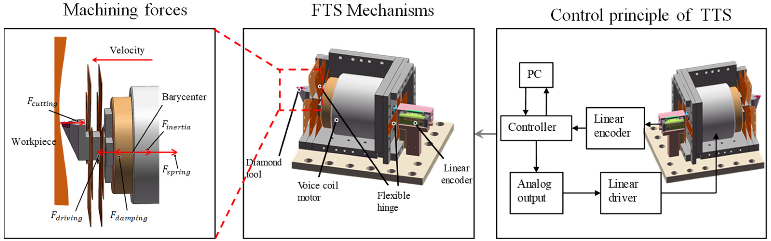
When the FTS device is used for diamond cutting, there will be a variety of machining forces including Lorentz force (
), spring force (
), inertia force (
), damping force (
), and cutting force (
). Lorentz force is the force generated by the voice coil motor that is used to drive the device to cut, so it can also be called the driving force. Spring forces are produced by the deformation of elastic hinges. The acceleration of the moving parts results in the presence of inertial forces. Damping forces are caused by the air and the inevitable friction within the device. Cutting force is the resistance to deformation generated during the process of material deformation and removal. Their relationship is complex. Due to the existence of the above forces, it is difficult to accurately obtain the cutting force of the interaction between the diamond tool and the workpiece surface along the axial direction of the system. The driving force, spring force, damping force, and inertia force of the device can be expressed as follows:
where
B represents the magnetic field intensity of the voice coil motor;
I represents the current passing through the voice coil motor;
L represents the length of one turn of the coil;
n represents the number of turns of the voice coil motor;
V represents the driving voltage signal used for the voice coil motor;
p represents the proportional coefficient between the driving voltage and the output current;
x represents the position of the tool;
k represents the spring coefficient of the elastic hinge;
c represents the sum of damping coefficients in the air and device; and
m represents the mass of the moving parts.
Utilizing the relationship between each machining force in the force equation, the cutting force can be calculated according to the machining signal (e.g., tool displacement signal) and control signal (e.g., drive voltage signal) in the machining process of the device, to achieve the estimation of cutting force. However, due to the uneven distribution of the magnetic field in the range of travel of the voice coil motor, the intensity of the magnetic field is related to the position of the tool, so the driving current and the driving force are not linear. The corresponding relationship between the two is a nonlinear relationship coupled with the displacement of the tool, which is shown in the following equation.
This relationship hinders accurate perception and estimation of cutting forces. At the same time, it is difficult to obtain the exact values of the spring coefficient and damping coefficient. Therefore, it is still difficult to estimate cutting forces accurately by the force balance equation.
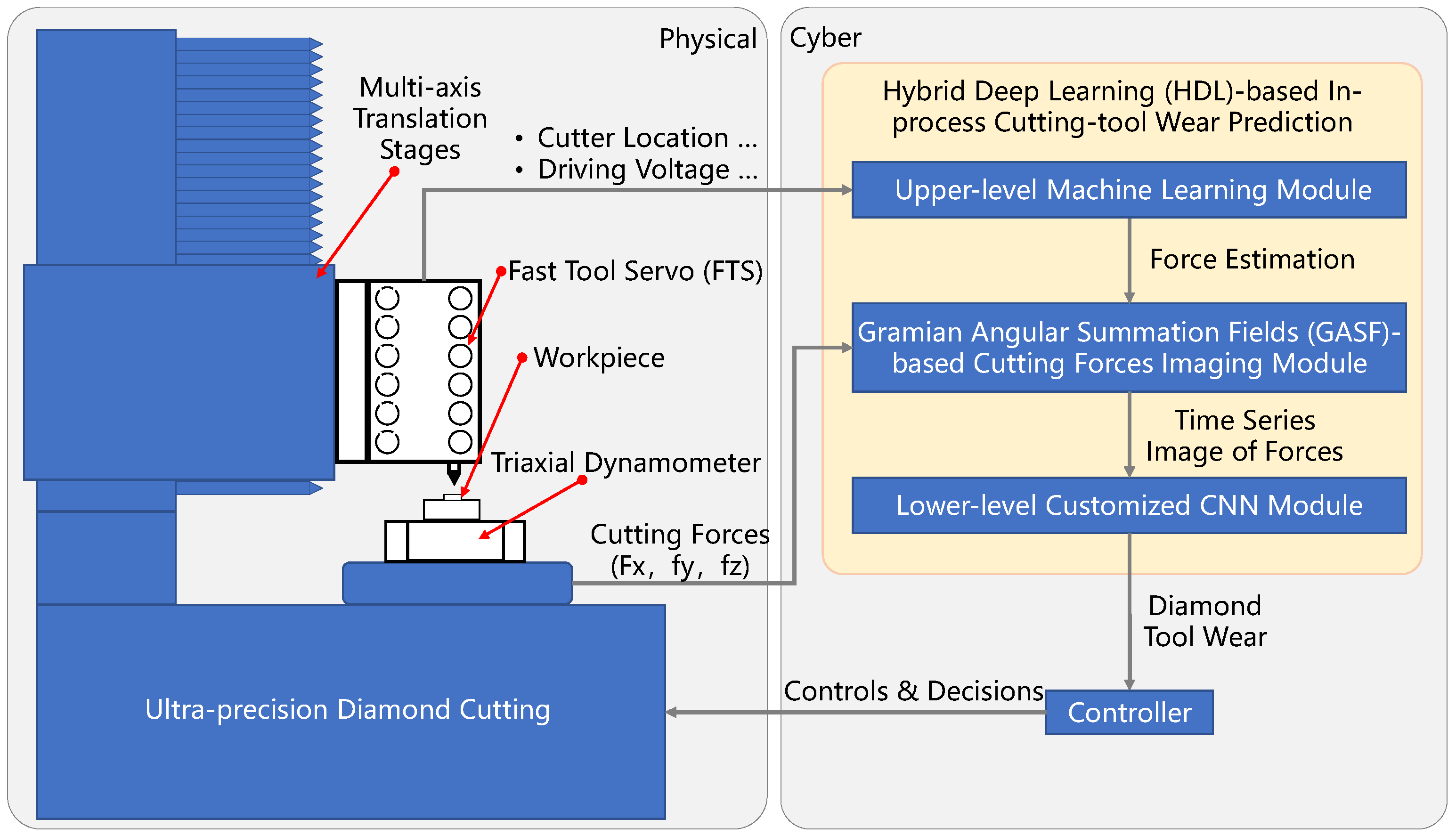
According to the above analysis, the corresponding relationship between the cutting force and machining signal, and the control signal of the FTS device can be obtained. To achieve an accurate estimation of cutting force in the machining process, this paper collects the machining signal, control signal, and cutting force in the machining process to train the neural network model, and thus realize an accurate estimation of cutting force.
To obtain the relationship between the extracted seven signal features and the actual cutting force (i.e., sample label), it is necessary to train the neural network to reveal the relationship. This paper uses a fully connected neural network as a machine learning model. The extracted seven features are input into the neural network through seven neurons in the input layer. After mapping between multiple hidden layers, the estimated cutting force value is output through a single neuron in the output layer. The structure of the fully connected neural network for cutting force estimation is shown in
Table 1.
4.2. Time Series Imaging of Cutting Forces
Since the convolutional neural network is sensitive to the spatial characteristics of the signal, time series imaging is carried out on the collected time series to convert the one-dimensional signal into a two-dimensional image, so that the result can be completed by time series imaging. The method adopted in this paper is the Gramian angular summation fields (GASF) method proposed by Wang et al. [
26], which can encode time series. In addition, the original time series obtained by this method can be reconstructed to understand how features are classified during the coding process. The image data are input into the HDL model.
The GASF method consists of two steps. First, the time series is represented in a polar coordinate system rather than in typical Cartesian coordinates. In this step, given
n observed values of a time series
, and then normalized
X, all values fall on the interval [−1, 1]:
The time series can be represented in polar coordinates by encoding the value as the angle of the corresponding cosine value, while the time is encoded as the radius in polar coordinates:
where
is a constant factor of the span of the regularized polar coordinate system. As time goes on, the corresponding values on the polar coordinate system move between different corners. This movement preserves the time relationship and makes it easy to identify time dependencies over different time intervals. This time correlation is expressed as follows:
GASF images provide a time-dependent method of preservation.
refers to the time interval
k superposition in the direction of the relative correlation. When the length of the time series is
n, the dimension of the GASF image obtained is
n ×
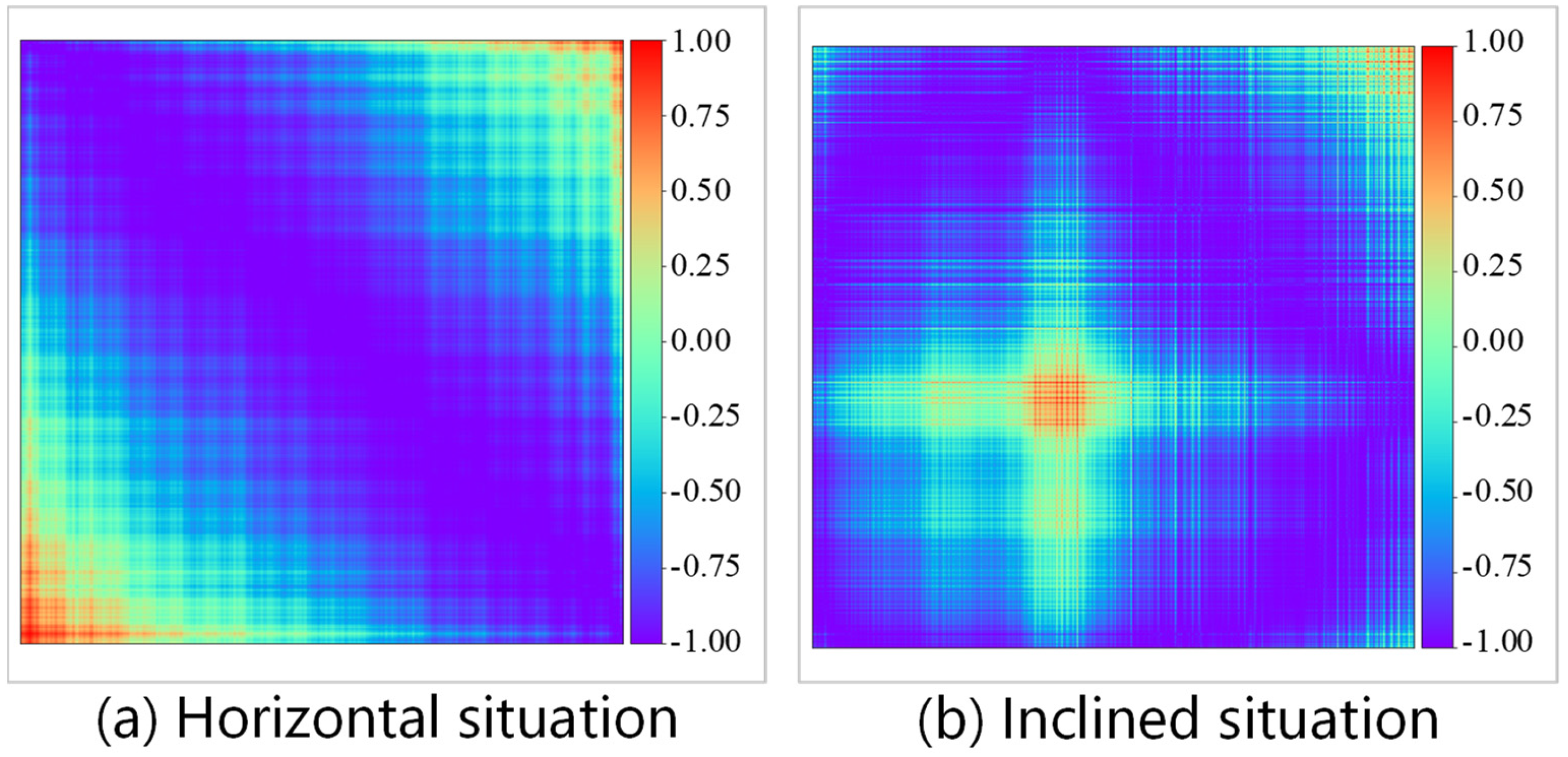
n. To reduce the size of the image, the piecewise aggregation approximation (PAA) technique can be applied to smooth the time series and reduce the number of sampling points. According to the sampling points of each group of experimental data, they were converted into 512 sampling points by the PAA method and then converted into two-dimensional images by the GASF method, each of whose size was 512 × 512. After output in the form of pictures, the image can be obtained as shown in
Figure 3.
Figure 3 shows the typical examples of the GASF images of the cutting force signals of non-wear diamond tools. The images reflect the signal distribution of the cutting force within 0.6 s sampling time. The images are on the diagonal symmetry and the distribution of cutting force can be easily found. With the powerful computing power of CNN, more hidden features can be excavated.
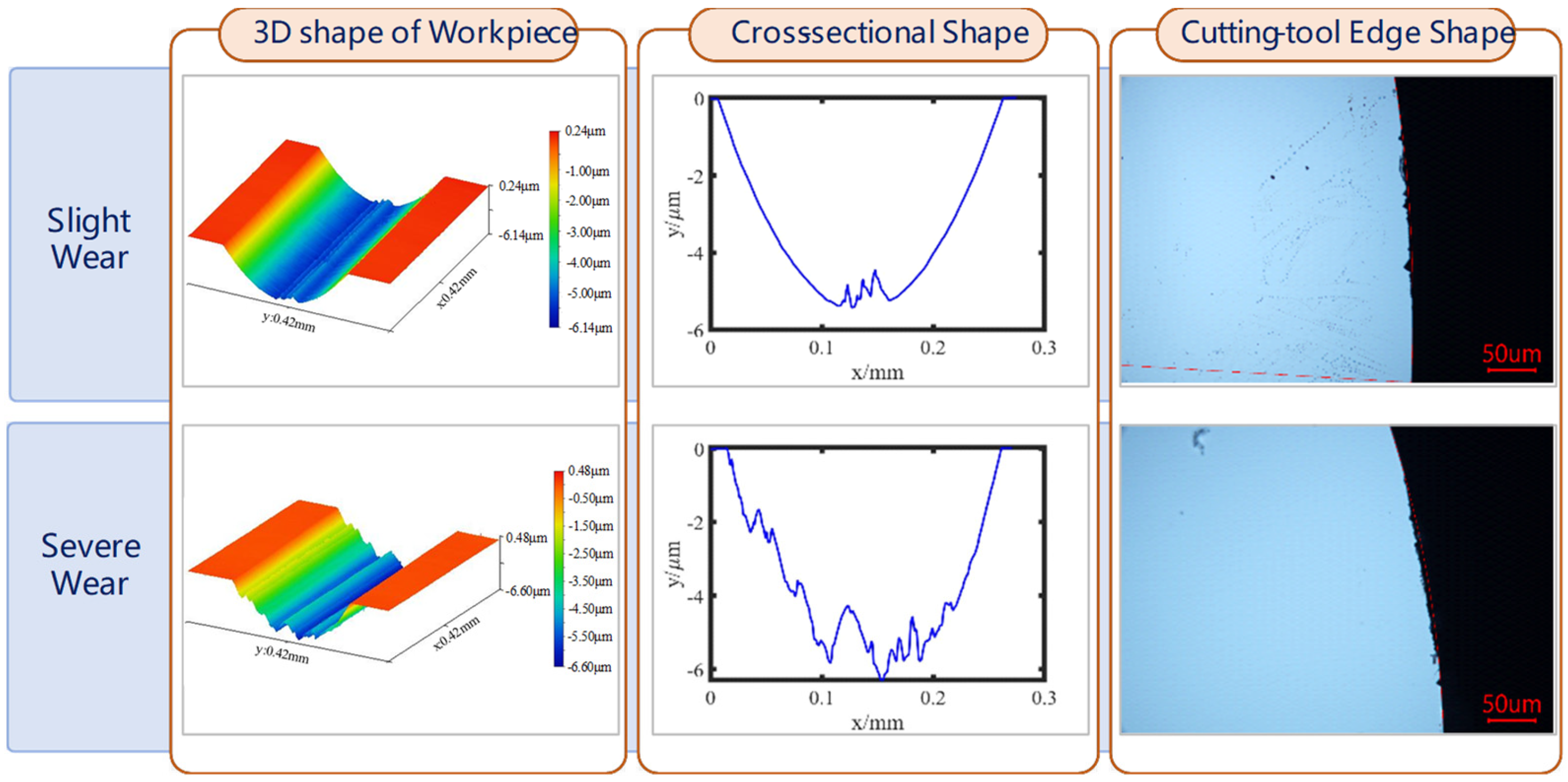
4.3. The Lower-Level Customized CNN Module for Diamond Tool Wear Prediction
Based on the principle of convolutional neural network and GASF images obtained by time series imaging, an HDL is proposed for diamond-tool wear prediction. At the same time, to classify the tool wear state, it is necessary to collect the machining data after tool wear. According to the morphology quality obtained by processing, the DTW can be divided into three states, namely, no wear, slight wear, and severe wear, as shown in
Figure 4. The structural parameters of the HDL model designed in this paper are shown in
Table 2.
The function of the convolutional layer is to extract high-dimensional features from the input data. The convolution kernel will carry out a cross-correlation operation between the input data and the weight coefficient in the convolution kernel, and then superimpose the corresponding bias quantity, to realize the convolution operation in this region, as follows:
where
represents the bias of the convolution kernel;
and
represent the input and output, respectively, of the convolution operation at the
level;
represents the size of the output data of
;
represents the value of the pixel point corresponding to row
i and column
j on the pixel image;
K represents the number of channels in the picture; and
f is the size of the convolution kernel.
The size of the convolutional kernel, the size of the convolutional step, and the number of filling layers are the parameters of the convolutional layer, which together affect the output size of the convolutional layer. The influence of the hyperparameter on the output size is formulated as follows:
where
represents the size of the output data of
; and
,
, and
represent the size of the convolution kernel, the convolution step, and the number of filling layers, respectively. Meanwhile, activation functions (sigmoid function, tanh function, and ReLU function) need to be added after the hidden layer, whose expression is as follows:
The function of the pooling layer is to reduce the dimension of the output data of the convolutional layer and carry out feature selection and information filtering.
Lp pooling adopted in this paper is expressed as follows:
where
,
have the same meaning as that of the convolution layer, and
p is a pre-specified parameter. When
p = 1, it is called average pooling. When
p goes to infinity, it is called max pooling. Meanwhile, the output data size of the pooling layer is similar to that of the convolutional layer, both of which are expressed by Equation (11).
The fully connected layer is the last part of the hidden layer of the convolutional neural network. In the fully connected layer, the two-dimensional image data will be flattened into a one-dimensional vector, thus losing the spatial topology, and then connected to other fully connected layers to transmit signals.
In the output layer, for image classification problems, the output layer generally uses normalized exponential function (softmax function) to output classification labels. In this paper, the expression of the softmax function is formulated as follows:
where
represents the predicted output value of the node in the output layer;
j indicates the number of output nodes; and
k represents the number of output nodes. Meanwhile, the number of output nodes represents the number of output categories.
expressed after the softmax output prediction probability value belongs to the probability value of each category, and its scope is [0, 1]. Softmax does not change the order of unnormalized predicted values, but only determines the probabilities assigned to each category. Meanwhile, according to maximum likelihood estimation, the cross-entropy loss function of the classification problem can be written as follows:
Among them,
and
refer to the actual tag values and forecasting values, respectively. After the above Equation (15) is substituted, it can be obtained as follows:
Using the loss function shown in the above Equations (4)–(12), its partial derivative concerning
can be obtained as follows:
The gradient of the loss function can be obtained by applying the above Equation (17), which can be used for the training and parameter updating of the neural network.
The HDL algorithm is divided into two parts, namely, excitation propagation and weight updating. Excitation propagation includes two steps, namely, forward propagation and back propagation. Firstly, the input data are fed into the network structure through forward propagation, and then the predicted output value is obtained by passing it to the output layer. Then the partial derivative of the loss function concerning the weight of each neuron is obtained through the back propagation to form its gradient concerning the weight vector.
In the weight updating step, the weight and bias coefficient of neurons are updated according to the calculated gradient. Since the gradient represents the direction of error increase, the gradient size needs to be subtracted during updating to reduce the error, which could be formulated as follows:
where
is the error calculated by the error function;
is the derivative of the activation function, namely, the ReLU function and softmax function; α stands for learning rate;
represents the predicted output value; and
l represents the label of the hidden layer.
The above formula can be used to update the parameters of neurons and realize the training of the HDL model.


