Adaptive Finite-Time Trajectory Tracking Control for Coaxial HAUVs Facing Uncertainties and Unknown Environmental Disturbances

Abstract

In this paper, the problems of system design, dynamic modeling, and trajectory tracking control of coaxial hybrid aerial underwater vehicles (HAUVs) with time-varying model parameters and composite marine environment disturbances are investigated. It is clear that a stable transition between different media remains a challenge in the practical implementation of amphibious tasks. For HAUVs, accurate dynamic modeling to describe complex dynamic variations during vehicle takeoff from underwater to air is a huge challenge. Meanwhile, due to the rapid changes in model parameters and the external environment, vehicles are likely to fall into the sea during the cross-domain process. An integrated continuous dynamic model considering hydrodynamic changes is established by introducing a linear switching coefficient during the process of trans-medium motion. A nonsingular fast terminal sliding-mode control (NFTSMC) algorithm combined with adaptive technology is used to design the position and attitude of the controller. With no previous knowledge of external interferences and lumped uncertainties of the HAUV, the adaptive NFTSMC (ANFTSMC) algorithm achieves the control objectives; at the same time, the inherent chattering problems of sliding mode control (SMC) are weakened. The finite-time stability of the global system is proven strictly using a series of mathematical derivations based on Lyapunov theory. The effect of the controller applied is analyzed through a series of simulations with representative working conditions. The results show that the proposed ANFTSMC can realize a “seamless” air–water trans-medium process, which proves the superiority and robustness of the proposed control algorithm.

1. Introduction

In recent decades, with the continuous development of marine resources across the world, countries have made important progress in the research and development of intelligent marine robotic technologies and developed various types of marine equipment, such as ocean observation buoys [1], underwater gliders (UGs) [2], unmanned surface vehicles (USVs) [3], unmanned underwater vehicles (UUVs) [4], and ocean unmanned aerial vehicles (UAVs) [5]. However, the main function of traditional marine robots is to realize surface water and underwater rescue operations, sampling, hydrological monitoring, intelligence gathering, and reconnaissance. It is impossible to realize the joint task of aerial, surface water, and underwater operations on the same platform. In order to realize multi-domain tasks, the common choice at present is the cooperative operation of different platforms, which not only wastes a large number of resources but also reduces the reliability of the whole system [6]. In recent years, scholars from various scientific research institutions have developed a new kind of ocean robot, the hybrid aerial underwater vehicle (HAUV) [7]. Combining the advantages of a UUV and a UAV, an HAUV is a new type of marine robot capable of performing various tasks in both water and air media, and research on HAUVs has gradually become a popular research topic in marine exploration equipment.

The concept of HAUVs can be traced back to the LPL flying submarine project proposed by Soviet engineer Ushakov in 1934 [8]. Since the LPL project, researchers have put forward a variety of different ideas for trans-medium vehicle schemes for different mission backgrounds and operational requirements. At present, many researchers focus on the structural design of HAUVs and attempt to explore practical and feasible solutions. According to the different structural forms of HAUVs, the existing research results can be roughly classified into three categories: fixed-wing design, multi-rotor design, and bionic design. In addition to these three main types, there is also a new type of HAUV designed to combine the benefits of both UAVs and UUVs [9]. HAUVs based on multi-rotor design are gradually winning the favor of researchers all over the world because of their significant advantages in vertical takeoff and landing and handling stability. In addition, the other most important factor is that a multi-rotor HAUV can navigate autonomously based on a set closed-loop control system. Due to the comprehensive advantages of multi-rotor HAUVs in terms of kinematic stability and maneuverability in the two media, HAUVs based on multi-rotor configurations are increasingly appearing.

At present, research on multi-rotor HAUVs mainly focuses on new configuration design, cross-medium system modeling analysis, and robust control system design and development. In 2014, P. Drews et al. conducted modeling and application scenario simulation research on their double-layer propeller HAUV [10]. In the initial study, the team used a simple gain-switching PD controller to verify the effectiveness of the modeling method through simulation. Researchers from Rutgers, the State University of New Jersey, designed a PID controller for their HAUV navigator that could adjust parameters based on the operating environment and verified the scheme through simulations and a pool test [11]. To circumvent the singular problems of Euler modeling, the team modeled the navigator’s attitude using the quaternion method and successfully performed high-mobility operations [12]. Researchers from the University of Auckland designed a PD controller for the Loon Copter and successfully implemented maneuvers for underwater navigation, underwater attitude adjustment, and taking off and landing across the water [13]. In 2016, a team at the China Air Force Engineering University proposed an active disturbance rejection control (ADRC) algorithm to achieve attitude control of a quadrotor HAUV operating near a water surface while considering ground effect [14]. However, this study only focused on the flight control of the HAUV under a complex flow field near the water surface and did not carry out a complete traverse-water maneuver. In 2018, to achieve vertical takeoff and landing of a double-layer HAUV in disturbed environments, the team further developed an adaptive sliding-mode control (ASMC) algorithm to achieve real-time estimation and compensation of system parameters and determine the impact of time-varying environments [15]. In 2019, Chen Yuqing et al. from Dalian Maritime University developed a tilting quadrotor HAUV with positive buoyancy and designed a sliding-mode controller (SMC) for the vehicle to realize stable control [16]. In 2021, the first HAUV with a coaxial rotor system and foldable propeller was proposed, and an MPC-SMC cascade controller was designed for it, which further improved the controller design through feedforward compensation for the influence of buoyancy [17]. In the same year, researchers from the Shanghai Maritime University designed a “fuzzy P+ID” attitude controller for their single-layer quadrotor HAUV prototype. Since the controller mechanism is simple and easy to adapt in traditional flight control systems, the authors experimentally demonstrated the effectiveness of the method [18]. Lu Di et al. modeled and analyzed the cross-medium process of a multi-rotor HAUV in detail, introduced a performance function into the HAUV control system for the first time, and adopted the adaptive dynamic surface control (ADSC) strategy to realize prescribed performance control in the trans-medium maneuver [19]. Subsequently, the team designed a dynamic surface controller based on a nonlinear disturbance observer (NDO) [20], which could accurately estimate the total uncertainty in real time and improve the robustness of the system. Recently, this team studied the instantaneous impact of periodic wave force acting on propellers and designed a second-order sliding-mode controller (SMC) to achieve a faster convergence rate and better robustness than traditional PID controllers [21]. A team from the Harbin Institute of Technology developed an amphibious multi-rotor UAV prototype [22], and the position and attitude controllers were established using an active disturbance rejection algorithm.

The HAUVs based on the multi-rotor configuration mentioned above have achieved fruitful research results. It is mentioned in references [23,24,25] that the arm of a multi-rotor vehicle causes a large disturbance to the body dynamics in the process of breaking through the water surface, which is the main shortcoming of the multi-rotor configuration. Coaxial systems offer a more compact structure and higher efficiency, as well as a greater payload and rotor area, than multi-rotor HAUV systems. A coaxial HAUV does not need to use the arm used by a multi-rotor HAUV, which reduces the forward projection area. Due to the application of the vector platform, a coaxial HAUV propeller does not need to accelerate and decelerate frequently during operation, thus reducing energy consumption and counteracting the gyroscopic effect of the propeller. Therefore, coaxial HAUVs have attracted the interest of researchers in recent years. In the literature, a missile-type trans-domain amphibious vehicle (TDAV) was proposed and successfully verified using a trans-medium motion flight test [26]. In another study, a coaxial HAUV with a folding propeller was proposed, and a cascaded predictive and sliding-mode controller was designed for the HAUV [17]. The new coaxial HAUV proved to have great potential for future development.

Based on the above research, we find that (1) it is very important to study an applicable HAUV modeling scheme and establish a reliable and accurate mathematical model for subsequent controller design work; (2) PD/PID and other linear controllers have a simple structure and are convenient for engineering applications. However, faced with a change in the environment, a linear controller cannot actively adjust the control output, which shows a lack of sufficient robustness; (3) Based on the switching of two working modes (water and air), sudden model changes can easily cause system instability.

Inspired by the above scholarly works and referencing existing coaxial aircraft, the authors developed a coaxial HAUV system in this work, as shown in Figure 1. The HAUV has two main modes of operation. When carrying an auxiliary float ball, it can be used as a drifting buoy. In this case, it is buoyant enough to float freely and does not need extra energy consumption to maintain the floating state. When the floating ball is abandoned, the gravity of the HAUV will be greater than its buoyancy (negative buoyancy stage). At this time, the HAUV can enter under the water for underwater sampling, underwater maneuvering, and other tasks. In order to collect a large range of hydrological data, the coaxial HAUV designed in this study needs to take off and land repeatedly on the water’s surface. To realize repeated cross-domain motion of the coaxial HAUV, a non-singular fast terminal sliding-mode controller (NFTSMC) based on the adaptive law was proposed. Compared with existing controller designs, the controller designed in this study improves response speed and realizes finite-time convergence of control errors. The adaptive law further improves the robustness of the controller to lumped uncertainties.

The rest of this paper is organized as follows: In Section 2, the design scheme and operation modes of the coaxial HAUV are explained, the modeling of the coaxial HAUV is analyzed in detail, and the dynamic modeling of the HAUV is presented in combination with our previous work. In Section 3, the design of the adaptive non-singular fast terminal sliding-mode controller (ANFTSMC) is explained, and its finite-time stability is proven using the Lyapunov method. In Section 4, the Simulink simulation results and explanation are provided to demonstrate the effectiveness of the proposed algorithm. Finally, Section 5 offers a brief conclusion and discussion as well as an outlook for future work plans.

The acronyms and full names used in this paper are described in

Table 1. The acronyms and full names used in this paper.

Acronyms	Full Name	Acronyms	Full Name
HAUVs	Hybrid aerial-underwater vehicles	ANFTSMC	Adaptive non-singular fast terminal sliding-mode controller
NFTSMC	Nonsingular fast terminal sliding mode control	AV	Unmanned aerial vehicle
SMC	sliding mode control	ADRC	Active disturbance rejection control
UG	Underwater gliders	ADSC	Adaptive dynamic surface control
USV	Unmanned surface vehicles	NDO	Nonlinear disturbance observer
UUV	Unmanned underwater vehicles	TDAV	Trans-domain amphibious vehicle

.

2. Dynamic Modeling of Trans-Medium Process

2.1. Preliminary

In this section, the operating mode of the coaxial HAUV developed by us is briefly introduced. In order to focus on the control problem of the HAUV’s cross-domain processes, we first analyzed the differences between the dynamic characteristics of the HAUV maneuvering underwater and in the air. Our goal is to provide hybrid dynamic models of trans-medium vehicles operating in the air, across domains, and under water. Therefore, the coaxial system’s dynamic model can be divided into three categories (underwater dynamics, trans-medium dynamics, and aerodynamics), which are organically unified by designing a linearized switch function.

As shown in Figure 1, the HAUV has two operating modes. It can maintain free floating for a long time to carry out long-term ocean observation tasks when carrying a float ball. When the float ball is abandoned, it can perform underwater maneuvering operations for underwater sampling and lurking tasks. In this study, the dynamic modeling and robust controller design for the most typical water–air cross-domain process (second operation mode) of the HAUV were investigated.

The symbols of the physical quantities related to modeling are shown in

Table 2. Related physical quantities and notation.

Variable Symbol	Physical Meaning	Variable Symbol	Physical Meaning
$o_b{x}_b{y}_b{z}_b$	body-fixed coordinate system	$V$	volume of watertight chamber
$o_e{x}_e{y}_e{z}_e$	inertial coordinate frame	$g$	acceleration of gravity
${\mathit{\eta }}_1={\left[\begin{array}{ccc}x& y& z\end{array}\right]}^{\mathrm{T}}$	position vector in inertial coordinate frame	${\left[\begin{array}{ccc}{x}_b& y_b& z_b\end{array}\right]}^{\mathrm{T}}$	center coordinate of buoyancy
${\mathit{\eta }}_2={\left[\begin{array}{ccc}\varphi & \theta & \psi \end{array}\right]}^{\mathrm{T}}$	attitude vector in inertial coordinate frame	$M_{bw}$	buoyancy torque
${\mathit{V}}_1={\left[\begin{array}{ccc}u& v& w\end{array}\right]}^{\mathrm{T}}$	linear velocities in the body-fixed frame	$\mathit{T}={\left[\begin{array}{ccc}{T}_x& T_y& T_z\end{array}\right]}^T$	control force
${\mathit{V}}_2={\left[\begin{array}{ccc}p& q& r\end{array}\right]}^{\mathrm{T}}$	angular velocities in the body-fixed frame	$\mathit{R}\left({\delta }_x,{\delta }_y\right)$	mapping transformation matrix
$m=diag\left[\begin{array}{ccc}m& m& m\end{array}\right]$	the HAUV’s body mass	$k_{\alpha }, k_{\beta }$	lift coefficients of the upper and lower propellers
$I=\left[\begin{array}{ccc}{I}_x& I_y& I_z\end{array}\right]$	the moments of inertia	$M_T={\left[\begin{array}{ccc}{u}_2& u_3& u_4\end{array}\right]}^T$	control torque
$m_a=diag\left[\begin{array}{ccc}{m}_{\dot{u}}& m_{\dot{v}}& m_{\dot{w}}\end{array}\right]$	added mass	$d$	lumped uncertainty and upper bound
$I_a=\left[\begin{array}{ccc}{I}_{\dot{p}}& I_{\dot{q}}& I_{\dot{r}}\end{array}\right]$	added moments of inertia	$V={\left[\begin{array}{ccc}{v}_x& v_y& v_z\end{array}\right]}^{\mathrm{T}}$	position virtual control
$m_w$, $I_w$	total mass and inertia	$x$	state vector
$k_s$, $k_{sa}$	linearization coefficient	$u_1$	total lift force
$K_{dw,} K_{da}$	drag coefficient matrices in underwater and air	${\varphi }_d$	expected roll
$F_{bw}$	buoyancy	${\theta }_d$	expected pitch
$\rho$	density of water	$\sigma$	lift loss coefficient of the lower propellers

.

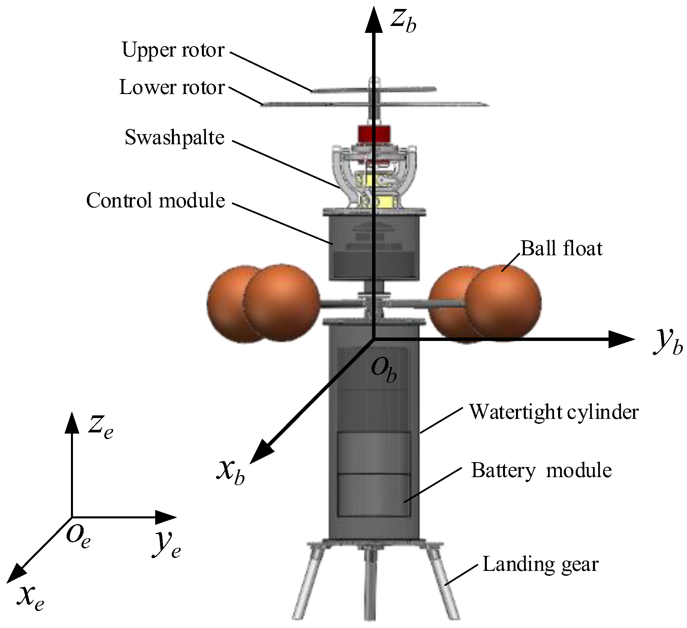
2.2. Reference Frame

In order to describe the motion of vehicles intuitively in three-dimensional space, two coordinate systems need to be defined as show in Figure 2 to establish a mathematical model. Since this study focuses on cross-domain phase motion, the z-axis direction in both the inertial coordinate system and the body-fixed coordinate system is defined as being upward. $o_b{x}_b{y}_b{z}_b$ is the body-fixed coordinate system, whose origin is defined at the center of gravity of the HAUV. The inertial coordinate frame $o_e{x}_e{y}_e{z}_e$ is an upper northeast coordinate system, and the $x_e{o}_e{y}_e$ plane coincides with the static water surface.

The position and the attitude vector of the vehicle are defined as ${\mathit{\eta }}_1={\left[\begin{array}{ccc}x& y& z\end{array}\right]}^{\mathrm{T}}$ and ${\mathit{\eta }}_2={\left[\begin{array}{ccc}\varphi & \theta & \psi \end{array}\right]}^{\mathrm{T}}$, respectively, in the earth-fixed reference frame. Furthermore, the horizontal motion of the HAUV is coupled to the roll and pitch, so the fuselage tilts during maneuvering, but it does not allow the fuselage to be flipped to avoid the singular problems of Euler angle modeling. ${\mathit{V}}_1={\left[\begin{array}{ccc}u& v& w\end{array}\right]}^{\mathrm{T}}$ and ${\mathit{V}}_2={\left[\begin{array}{ccc}p& q& r\end{array}\right]}^{\mathrm{T}}$ are defined as the linear and angular velocities, respectively, in the body-fixed frame.

$${\mathit{R}}_1=\left[\begin{array}{ccc}\mathrm{c}\theta \cdot \mathrm{c}\psi & \mathrm{s}\varphi \cdot \mathrm{s}\theta \cdot \mathrm{c}\psi -\mathrm{c}\varphi \cdot \mathrm{s}\psi & \mathrm{c}\varphi \cdot \mathrm{s}\theta \cdot \mathrm{c}\psi +\mathrm{s}\varphi \psi \\ \mathrm{c}\theta \cdot \mathrm{s}\psi & \mathrm{s}\varphi \cdot \mathrm{s}\theta \cdot \mathrm{s}\psi +\mathrm{c}\varphi \cdot \mathrm{c}\psi & \mathrm{c}\varphi \cdot \mathrm{s}\theta \cdot \mathrm{s}\psi -\mathrm{s}\varphi c\psi \\ -\mathrm{s}\theta & \mathrm{s}\varphi \cdot c\theta & \mathrm{c}\varphi \cdot c\theta \end{array}\right]$$

(1)

$${\mathit{R}}_2=\left[\begin{array}{ccc}1& \mathrm{s}\varphi \cdot \mathrm{t}\theta & \mathrm{c}\varphi \cdot \mathrm{t}\theta \\ 0& \mathrm{c}\varphi & -\mathrm{s}\varphi \\ 0& \mathrm{s}\varphi /\mathrm{c}\theta & \mathrm{c}\varphi /\mathrm{c}\theta \end{array}\right]$$

(2)

Here, c(·), s(·), and t(·) denote cos(·), sin(·), and tan(·), respectively. It should be noted that ${\mathit{R}}_1$ is an orthogonal matrix, so we have ${\mathit{R}}_1^{-1}={\mathit{R}}_1^{\mathrm{T}}$. Therefore, the kinematic equation of HAUV is as follows:

$$\begin{gathered} {\dot{\mathit{\eta }}}_1={\mathit{R}}_1{\mathit{V}}_1 \\ {\dot{\mathit{\eta }}}_2={\mathit{R}}_2{\mathit{V}}_2 \end{gathered}$$

(3)

During the cross-domain process, the HAUV does not carry out severe maneuvering, so reasonable assumptions can be made to simplify the dynamic model for the convenience of controller design. The following assumptions are made:

Assumption 1. 

The mass of the HAUV is evenly distributed over the cylindrical watertight cabin, and the tank body is rigidly symmetric with respect to the three coordinate planes.

Assumption 2. 

Due to the small maneuvering speed, the Coriolis term of translational motion and complex coupling hydrodynamic parameters can be ignored.

2.3. Dynamic Modeling

Most of the operating conditions of the HAUV are in the state of underwater navigation or air flight, and the cross-domain maneuvering process is very short. Purely from the perspective of dynamics, the HAUV has the most force action during underwater movement, which is affected by gravity, buoyancy, propeller thrust and drag, and corresponding torque. When the HAUV breaks through the water surface and enters the flight state, its dynamics change greatly. In order to organically unify the whole dynamic change process, the HAUV can be modeled as a mixed system, and the dynamics of the HAUV can be defined according to the operating environmental medium (air or water).

2.3.1. Added Mass

Since the coaxial HAUV can be considered symmetric, both the mass matrix and the inertia matrix of the HAUV are simplified to their principal diagonal matrices based on related literature [16]. $m=diag\left[\begin{array}{ccc}m& m& m\end{array}\right]$ and $I=\left[\begin{array}{ccc}{I}_x& I_y& I_z\end{array}\right]$ are the HAUV’s body mass and the moments of inertia, respectively. The fluid around the HAUV is moved by the HAUV as it navigates in the water. The mass of this attached fluid is called added mass (inertia), and it is proportional to the acceleration and angular acceleration of the object. According to Assumption 1, the added mass matrix is also diagonal and can be described as $m_a=diag\left[\begin{array}{ccc}{m}_{\dot{u}}& m_{\dot{v}}& m_{\dot{w}}\end{array}\right]$, $I_a=\left[\begin{array}{ccc}{I}_{\dot{p}}& I_{\dot{q}}& I_{\dot{r}}\end{array}\right]$. $m_w$ and $I_w$ are the total mass and inertia of the vehicle, respectively.

$$\begin{array}{l}{m}_w=m+k_s{m}_a\\ I_w=I+k_s{I}_a\end{array}$$

(4)

Remark 1. 

Based on the design in reference [15], we introduce a linearization coefficient to approximate the variation trend of additional variables. The significance of setting a linear switching coefficient is to avoid the jump mutation of the medium density in the cross-media stage, which approximately represents the variation trend of additional variables and links the HAUV’s underwater maneuvering and aerial maneuvering processes together. The linearization coefficient $k_s$ can be expressed as follows:

$$k_s=\{\begin{array}{c}0,z\ge h/2\\ \left(1/2-z/h\right),-h/2<z<h/2\\ 1,z\le -h/2\end{array}$$

(5)

where $h$ is the height of the vehicle. Obviously, $k_s$ represents the approximate variation law of the hydrodynamic force of the vehicle, and the aerodynamic variation trend is represented by $k_{sa}$, which is expressed as $k_{sa}=1-k_s$.

2.3.2. Drag Force and Moment

Because water is much denser than air, the resistance of vehicles when moving in water is also much greater than that in air. Although the drag coefficient is related to the vehicle’s characteristic area, angle of attack, velocity, and fluid properties, we consider the drag coefficient a constant in the modeling for simplicity. The drag and drag moment can be considered to be approximately proportional to the square of the vehicle’s linear velocity and angular velocity:

$$F_{rw}={\left[\begin{array}{ccc}\left(k_s{k}_{xw}+k_{sa}{k}_{xa}\right)\left|\dot{x}\right|\dot{x}& \left(k_s{k}_{yw}+k_{sa}{k}_{ya}\right)\left|\dot{y}\right|\dot{y}& \left(k_s{k}_{zw}+k_{sa}{k}_{za}\right)\left|\dot{z}\right|\dot{z}\end{array}\right]}^{\mathrm{T}}$$

(6)

$$M_{rw}={\left[\begin{array}{ccc}\left(k_s{k}_{\varphi w}+k_{sa}{k}_{\varphi a}\right)\left|\dot{\varphi }\right|\dot{\varphi }& \left(k_s{k}_{\theta w}+k_{sa}{k}_{\theta a}\right)\left|\dot{\theta }\right|\dot{\theta }& \left(k_s{k}_{\psi w}+k_{sa}{k}_{\psi a}\right)\left|\dot{\psi }\right|\dot{\psi }\end{array}\right]}^{\mathrm{T}}$$

(7)

where $K_{{}_{dw}}=diag\left[\begin{array}{cccccc}{k}_{{}_{xw}}& k_{{}_{yw}}& k_{{}_{zw}}& k_{{}_{\varphi w}}& k_{{}_{\theta w}}& k_{{}_{\psi w}}\end{array}\right]$ represent the drag coefficient matrices in water, respectively, and $K_{{}_{da}}=diag\left[\begin{array}{cccccc}{k}_{{}_{xa}}& k_{{}_{ya}}& k_{{}_{za}}& k_{{}_{\varphi a}}& k_{{}_{\theta a}}& k_{{}_{\psi a}}\end{array}\right]$ represent the drag coefficient matrices in air.

Remark 2. 

It is worth noting that the damping coefficient depends on the Reynolds number and the projected area. A detailed discussion on the drag coefficient can be found in reference [27], where only the main factors of drag are considered. Finally, drastic maneuvers are not considered in translational motion, and the Coriolis forces in translational motion are usually not considered.

2.3.3. Restoring Force and Moment

The amount of buoyancy equal to the weight of water expelled by the HAUV is calculated based on Archimedes’ principle:

$$F_{bw}=k_s\rho Vg$$

(8)

where $\rho$, $V$, and $g$ represent the density of water, the volume of the watertight chamber, and the acceleration of gravity, respectively. It is worth noting that as the HAUV crosses the water–air boundary, we approximately assume that the change $V$ is still linear.

Since the origin of the body coordinate system is defined at the center of mass of the HAUV, the heavy moment is not considered. If the center coordinate of buoyancy is defined as ${\left[\begin{array}{ccc}{x}_b& y_b& z_b\end{array}\right]}^{\mathrm{T}}$, then the buoyancy torque can be expressed as follows:

$$M_{bw}=-F_{bw}\left[\begin{array}{c}{z}_{b}s\varphi c\theta -y_{b}c\varphi c\theta \\ x_{b}c\varphi c\theta +z_{b}s\theta \\ -y_{b}s\theta -x_{b}s\varphi c\theta \end{array}\right]$$

(9)

Remark 3. 

To improve the maneuverability of the coaxial HAUV, it is designed to be slightly less buoyant than gravity when not equipped with a float ball. In this mode of operation, the coaxial HAUV can maneuver under the water. In addition, according to the basic knowledge about the initial stability of a floating body using the ship principle, the stability of a floating body is closely related to its initial metacentric position. Meanwhile, the position of the metacenter is related to the positions of the center of buoyancy and the center of gravity, which makes it difficult to calculate the recovery moment accurately. In order to further simplify the dynamic model, the recovery torque generated by the buoyancy force is regarded as an external interference, and its calculation is not considered.

2.3.4. Control Force and Moment

The propellers used in HAUVs are usually aviation propellers, and previous experimental studies have shown that air propellers can be used for underwater propulsion to some extent. The coaxial HAUV is equipped with two propellers and a swash plant. The control force and torque generated by them can be expressed as follows [17,28,29]:

$$\mathit{T}=\left[\begin{array}{c}{T}_x\\ T_y\\ T_z\end{array}\right]=\mathit{R}\left({\delta }_x,{\delta }_y\right)\left[\begin{array}{c}0\\ 0\\ k_{\alpha }{\omega }_1^2+\sigma k_{\beta }{\omega }_2^2\end{array}\right]$$

(10)

$$\mathit{R}\left({\delta }_x,{\delta }_y\right)=\left[\begin{array}{ccc}\cos {\delta }_y& -\sin {\delta }_y\sin {\delta }_x& -\sin {\delta }_y\cos {\delta }_x\\ 0& \cos {\delta }_x& -\sin {\delta }_x\\ \sin {\delta }_y& \cos {\delta }_y\sin {\delta }_y& \cos {\delta }_x\cos {\delta }_y\end{array}\right]$$

(11)

$${\mathit{M}}_T=\left[\begin{array}{c}{u}_2\\ u_3\\ u_4\end{array}\right]=\left[\begin{array}{c}-d\sin {\delta }_x\left(k_{\alpha }{\omega }_1^2+\sigma k_{\beta }{\omega }_2^2\right)\\ -d\sin {\delta }_y\cos {\delta }_x\left(k_{\alpha }{\omega }_1^2+\sigma k_{\beta }{\omega }_2^2\right)\\ {\gamma }_{\alpha }{\omega }_1^2+{\gamma }_{\beta }{\omega }_2^2\end{array}\right]$$

(12)

where $k_{\alpha }$ and $k_{\beta }$ are the lift coefficients of the upper and lower propellers, respectively; $\sigma$ is the lift loss coefficient of the lower propellers; d is the distance from the propeller center to the center of mass; $\mathit{R}\left({\delta }_x,{\delta }_y\right)$ represents the mapping transformation matrix of propeller thrust to the HAUV body; and ${\delta }_x$ and ${\delta }_y$ are the deflection angles of the swash plant.

Remark 4. 

From the perspective of actual flight control and considering that the swash platform angles are very small, we can obtain $\cos {\delta }_x\approx 1$, $\cos {\delta }_y\approx 1$, $\sin {\delta }_x\approx {\delta }_x\approx 0$, and $\sin {\delta }_y\approx {\delta }_y\approx 0$. The control actuator model can be simplified, and the lateral effects caused by $T_x$ and $T_x$ in (10) are negligible compared to the main thrust force $T_z$. For convenience, let us redefine $T_z$ to be $u_1$.

2.3.5. Wind, Wave, and Current Complex Interference Analysis

When the coaxial HAUV traverses the water surface in cross-domain maneuvering, its body will be subjected to multiple marine environmental disturbances, such as wind gusts, waves, and ocean currents. The perturbation of the HAUV at the water–air boundary surface has been discussed in reference 1, but the actual marine environment is difficult to simulate. To test the robustness and effectiveness of the control algorithm, random time-varying sine or cosine functions are generally used to simulate the marine environment in the literature to realize AUV control. This approximation of the marine environment is reasonable because wind, waves, and currents are also random and irregular in the real environment. In addition to the interference of the external environment, some simplified assumptions are adopted in the modeling process, which makes the established model not strict and accurate, and there are uncertainties in the model. Considering that an actual underwater environment is more complex, the lumped uncertainties are set as follows:

$$\begin{gathered} d_x=0.2\times \left(cos\left(0.4t\right)+k_s\right),d_y=0.2\times \left(sin\left(0.5t\right)+k_s\right),d_z=0.2\times \left(sin\left(0.7t\right)+k_s\right) \\ {d}_{\varphi }=0.2\times \left(cos\left(0.4t\right)+k_s\right),d_{\theta }=0.2\times \left(sin\left(0.5t\right)+k_s\right),d_{\psi }=0.2\times \left(sin\left(0.7t\right)+k_s\right) \end{gathered}$$

(13)

2.4. The HAUV Dynamic Model

Based on the above analysis, a dynamic model can be obtained according to the Newton–Euler formula. Owing to the underactuated characteristics of the coaxial HAUV, the coaxial HAUV model is divided into a double-ring structure [30], namely a translation subsystem and a rotation subsystem, as shown in the following formulae:

$$\{\begin{array}{c}{\dot{x}}_1=x_2\hfill \\ {\dot{x}}_2=x_4{x}_6\left(I_{yw}-I_{zw}\right)/I_{xw}+u_2/I_{xw}-\left(k_s{k}_{\varphi w}+k_{sa}{k}_{\varphi a}\right)\left|x_2\right|x_2/I_{xw}+d_{\varphi }\hfill \\ {\dot{x}}_3=x_4\hfill \\ {\dot{x}}_4=x_2{x}_6\left(I_{zw}-I_{xw}\right)/I_{yw}+u_3/I_{yw}-\left(k_s{k}_{\theta w}+k_{sa}{k}_{\theta a}\right)\left|x_4\right|x_4/I_{yw}+d_{\theta }\hfill \\ {\dot{x}}_5=x_6\hfill \\ {\dot{x}}_6=x_2{x}_4\left(I_{xw}-I_{yw}\right)/I_{zw}+u_4/I_{zw}-\left(k_s{k}_{\psi w}+k_{sa}{k}_{\psi a}\right)\left|x_6\right|x_6/I_{zw}+d_{\psi }\hfill \end{array}$$

(14a)

$$\{\begin{array}{c}{\dot{x}}_7=x_8\hfill \\ {\dot{x}}_8=u_1/m_w\left(\mathrm{c}{x}_1\cdot \mathrm{s}{x}_3\cdot \mathrm{c}{x}_3+\mathrm{s}{x}_1\cdot \mathrm{s}{x}_5\right)-\left(k_s{k}_{xw}+k_{sa}{k}_{xa}\right)\left|x_8\right|x_8/m_w+d_x\hfill \\ {\dot{x}}_9=x_{10}\hfill \\ {\dot{x}}_{10}=u_1/m_w\left(\mathrm{c}{x}_1\cdot \mathrm{s}{x}_3\cdot \mathrm{s}{x}_5-\mathrm{s}{x}_1\cdot \mathrm{c}{x}_5\right)-\left(k_s{k}_{yw}+k_{sa}{k}_{ya}\right)\left|x_{10}\right|x_{10}/m_w+d_y\hfill \\ {\dot{x}}_{11}=x_{12}\hfill \\ {\dot{x}}_{12}=u_1/m_w\mathrm{c}{x}_1\cdot \mathrm{c}{x}_3-g+k_s{F}_{bw}/m_w-\left(k_s{k}_{zw}+k_{sa}{k}_{za}\right)\left|x_{12}\right|x_{12}/m_w+d_z\hfill \end{array}$$

(14b)

where ${x=[\varphi ,\dot{\varphi },\theta ,\dot{\theta },\psi ,\dot{\psi },x,\dot{x},y,\dot{y},z,\dot{z}]}^{\mathrm{T}}\in R^{12}$ is defined as a state vector. The rotational dynamic model and the translational dynamic model can be considered second-order systems with perturbations. $d={\left[\begin{array}{cccccc}{d}_x& d_y& d_z& d_{\varphi }& d_{\theta }& d_{\psi }\end{array}\right]}^{\mathrm{T}}$ is the lumped uncertainty, including model uncertainty and environmental disturbance.

Remark 5. 

Since the vehicle body can always maintain a small attitude-angle change operation during the vertical takeoff and landing process, the small angle assumption can be further made. Based on the small angle hypothesis, we have reasonably simplified the mathematical model [19].

Assumption 3. 

Obviously, lumped uncertainties are not divergent, and there exists a positive number satisfying the inequation, $\Vert d\Vert \le D$, where $D$ is the upper bound of lumped uncertainty. $D$ can be expressed as $D\le a_{0i}+a_{1i}\left|e_i\right|+a_{2i}\left|e_{i+1}\right|,i=1,3,5,\cdots ,11$.

Since the whole system is divided into inner and outer loops, the position of virtual control is defined as $V={\left[\begin{array}{ccc}{v}_x& v_y& v_z\end{array}\right]}^{\mathrm{T}}$.

The virtual position controller is designed according to Equation (15) [31]:

$$\left[\begin{array}{c}{v}_x\\ v_y\\ v_z\end{array}\right]=\left[\begin{array}{c}{u}_1/m_w\left(\mathrm{c}\varphi \cdot \mathrm{s}\theta \cdot \mathrm{c}\psi +\mathrm{s}\varphi \cdot \mathrm{s}\psi \right)\\ u_1/m_w\left(\mathrm{c}\varphi \cdot \mathrm{s}\theta \cdot \mathrm{s}\psi -\mathrm{s}\varphi \cdot \mathrm{c}\psi \right)\\ u_1/m_w\mathrm{c}\varphi \cdot \mathrm{c}\theta -g+k_s{F}_{bw}/m_w\end{array}\right]$$

(15)

Hence, the expected roll and pitch can be calculated through the virtual position controller. Meanwhile, the total lift force can be calculated as follows:

$$\{\begin{array}{l}{u}_1=m\sqrt{v_x^2+v_y^2+{\left(v_z+g-k_s{F}_{bw}/m_w\right)}^2}\hfill \\ {\varphi }_d={\tan }^{-1}\left(\cos {\theta }_d\left(\frac{v_x\sin {\psi }_d-v_y\cos {\psi }_d}{v_z+g-k_s{F}_{bw}/m_w}\right)\right)\hfill \\ {\theta }_d={\tan }^{-1}\left(\frac{v_x\cos {\psi }_d+v_y\sin {\psi }_d}{v_z+g-k_s{F}_{bw}/m_w}\right)\hfill \end{array}$$

(16)

3. Finite-Time ANFTSMC Design

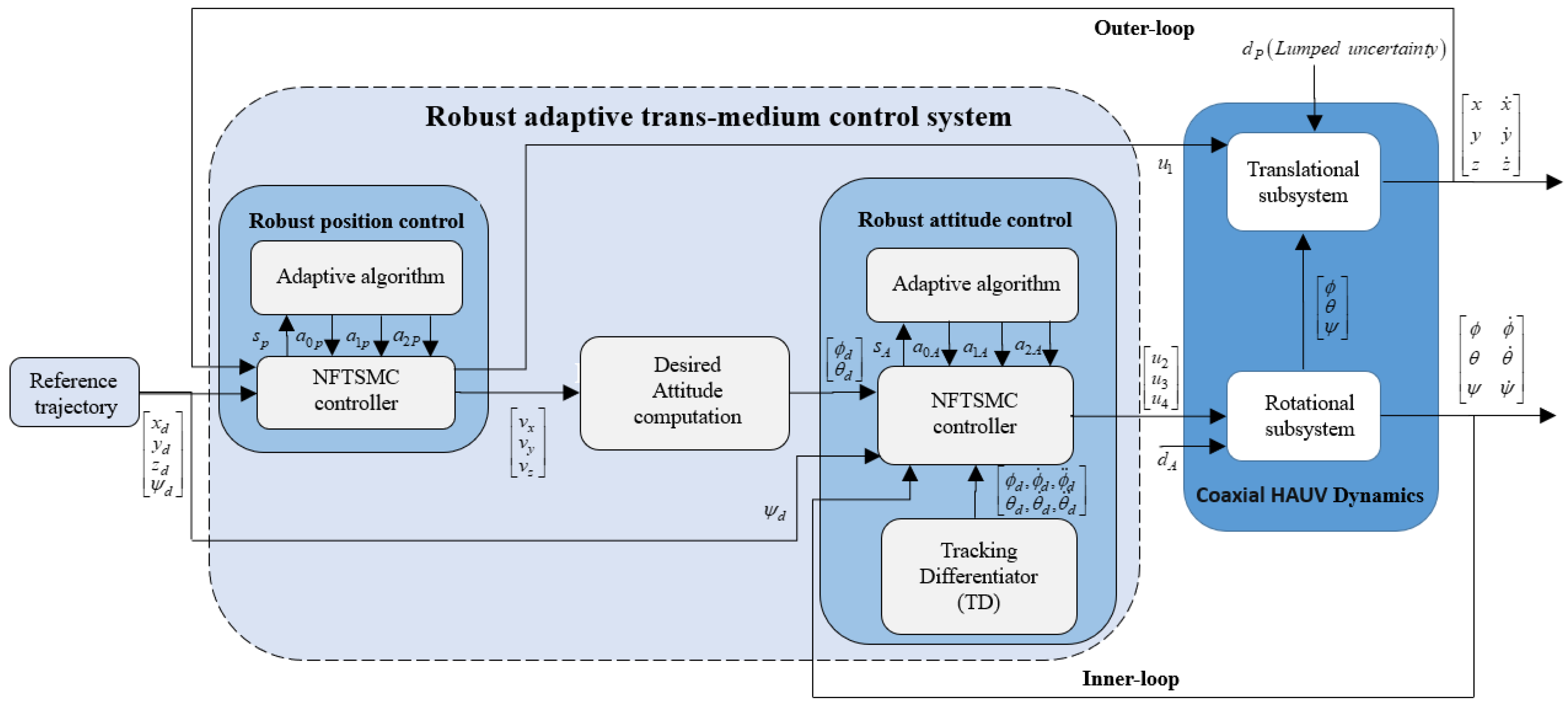
3.1. Controller Design Methodology for HAUV

This section mainly presents a nonlinear control scheme for the HAUV’s cross-domain process, which provides a reliable and robust control method for air and underwater navigation and HAUV water–air traversing maneuvers. The coaxial HAUV studied in this paper is a typical underactuated system that is faced with nonlinear and strong coupling characteristics and complex environmental disturbances. Because sliding-mode variable structure control has strong robustness in the presence of system parameter perturbations and unknown external disturbances, sliding-mode control is used to design the position controller and the attitude controller of the vehicle. Figure 3 shows the block diagram of the coaxial HAUV’s control logic. As shown in Figure 3, the control logic consists of two loops: the inner loop (attitude) and the outer loop (position). An ANFTSMC is designed for the outer loop and the inner loop, respectively. The controller achieves a faster convergence rate and can estimate the unknown upper bound of uncertainty by using an adaptive algorithm, which improves the robustness of the coaxial HAUV’s control system to lumped uncertainty.

The main content of this section is to discuss and analyze the design of the controller system outlined for the coaxial HAUV. The controller is designed with NFTSMC technology for the coaxial HAUV’s translation subsystem and rotation subsystem. Under this control framework, external disturbances and system uncertainties are estimated online in real time by using an adaptive algorithm. The controller can ensure that tracking errors gradually converge to zero in a finite amount of time.

3.2. Controller Design Procedure

3.2.1. NFTSMC Design

Below, we first define tracking errors as follows:

$$\begin{array}{l}{\left[\begin{array}{ccc}{e}_1& e_3& e_5\end{array}\right]}^{\mathrm{T}}={\left[\begin{array}{ccc}\varphi -{\varphi }_d& \theta -{\theta }_d& \psi -{\psi }_d\end{array}\right]}^{\mathrm{T}}\\ {\left[\begin{array}{ccc}{e}_2& e_4& e_6\end{array}\right]}^{\mathrm{T}}={\left[\begin{array}{ccc}\dot{\varphi }-{\dot{\varphi }}_d& \dot{\theta }-{\dot{\theta }}_d& \dot{\psi }-{\dot{\psi }}_d\end{array}\right]}^{\mathrm{T}}\end{array}$$

(17)

$$\begin{array}{l}{\left[\begin{array}{ccc}{e}_7& e_9& e_{11}\end{array}\right]}^{\mathrm{T}}={\left[\begin{array}{ccc}x-x_d& y-y_d& z-z_d\end{array}\right]}^{\mathrm{T}}\\ {\left[\begin{array}{ccc}{e}_8& e_{10}& e_{12}\end{array}\right]}^{\mathrm{T}}={\left[\begin{array}{ccc}\dot{x}-{\dot{x}}_d& \dot{y}-{\dot{y}}_d& \dot{z}-{\dot{z}}_d\end{array}\right]}^{\mathrm{T}}\end{array}$$

(18)

where ${\left[\begin{array}{ccc}{x}_d& y_d& z_d\end{array}\right]}^{\mathrm{T}}$ and ${\left[\begin{array}{ccc}{\varphi }_d& {\theta }_d& {\psi }_d\end{array}\right]}^{\mathrm{T}}$ are the desired position and attitude angle, respectively. The sliding surfaces of the translation subsystem and the rotation subsystem are introduced as ${\mathit{S}}_A={\left[\begin{array}{ccc}{S}_1& S_3& S_5\end{array}\right]}^{\mathrm{T}}$ and ${\mathit{S}}_P={\left[\begin{array}{ccc}{S}_7& S_9& S_{11}\end{array}\right]}^{\mathrm{T}}$ [32,33,34].

$$\begin{array}{l}{s}_1=e_1+b_1{\left|e_1\right|}^{{\alpha }_1}sign\left(e_1\right)+b_2{\left|e_2\right|}^{{\beta }_1}sign\left(e_2\right)\hfill \\ s_3=e_3+b_3{\left|e_3\right|}^{{\alpha }_3}sign\left(e_3\right)+b_4{\left|e_4\right|}^{{\beta }_3}sign\left(e_4\right)\hfill \\ s_5=e_5+b_5{\left|e_5\right|}^{{\alpha }_5}sign\left(e_5\right)+b_6{\left|e_6\right|}^{{\beta }_5}sign\left(e_6\right)\hfill \end{array}$$

(19a)

$$\begin{array}{l}{s}_7=e_7+b_7{\left|e_7\right|}^{{\alpha }_7}sign\left(e_7\right)+b_8{\left|e_8\right|}^{{\beta }_7}sign\left(e_8\right)\hfill \\ s_9=e_9+b_9{\left|e_9\right|}^{{\alpha }_9}sign\left(e_9\right)+b_{10}{\left|e_{10}\right|}^{{\beta }_9}sign\left(e_{10}\right)\hfill \\ s_{11}=e_{11}+b_{11}{\left|e_{11}\right|}^{{\alpha }_{11}}sign\left(e_{11}\right)+b_{12}{\left|e_{12}\right|}^{{\beta }_{11}}sign\left(e_{12}\right)\hfill \end{array}$$

(19b)

Here, $b_i,b_{i+1}(i=1,3,5,7,9,11)$ are positive constants, and $1<{\beta }_i<2$, ${\alpha }_i>{\beta }_i$. The time derivative of the sliding surfaces can be estimated as follows:

$${\dot{s}}_i=e_{i+1}+{\alpha }_i{b}_i{\left|e_i\right|}^{{\alpha }_i-1}{e}_{i+1}+{\beta }_i{b}_{i+1}{\left|e_{i+1}\right|}^{{\beta }_i-1}{\dot{e}}_{i+1}$$

(20)

By setting ${\dot{s}}_i=0$, an equivalent control term can be obtained. Then, the equivalent controller equations of attitude and position are shown in Equations (21a) and (21b), respectively:

$$\begin{array}{cc}\hfill U_{2eq}& =\left(-x_4{x}_6\left(I_{yw}-I_{zw}\right)+\left(k_s{k}_{\varphi w}+k_{sa}{k}_{\varphi a}\right)\left|x_2\right|x_2\right)\hfill \\ & +I_{xw}\left({\ddot{\varphi }}_d-\frac{1}{{\beta }_1{b}_2}{\left|e_2\right|}^{2-{\beta }_1}\left(1+{\alpha }_1{b}_1{\left|e_1\right|}^{{\alpha }_1-1}\right)sign\left(e_2\right)\right)\hfill \\ \hfill U_{3eq}& =\left(-x_2{x}_6\left(I_{zw}-I_{xw}\right)+\left(k_s{k}_{\theta w}+k_{sa}{k}_{\theta a}\right)\left|x_4\right|x_4\right)\hfill \\ & +I_{yw}\left({\ddot{\theta }}_d-\frac{1}{{\beta }_3{b}_4}{\left|e_4\right|}^{2-{\beta }_3}\left(1+{\alpha }_3{b}_3{\left|e_3\right|}^{{\alpha }_3-1}\right)sign\left(e_4\right)\right)\hfill \\ \hfill U_{4eq}& =\left(-x_2{x}_4\left(I_{xw}-I_{yw}\right)+\left(k_s{k}_{\psi w}+k_{sa}{k}_{\psi a}\right)\left|x_6\right|x_6\right)\hfill \\ & +I_{zw}\left({\ddot{\psi }}_d-\frac{1}{{\beta }_5{b}_6}{\left|e_6\right|}^{2-{\beta }_5}\left(1+{\alpha }_5{b}_5{\left|e_5\right|}^{{\alpha }_5-1}\right)sign\left(e_6\right)\right)\hfill \end{array}$$

(21a)

$$\begin{array}{c}{v}_{xeq}=\left(k_s{k}_{xw}+k_{sa}{k}_{xa}\right)\left|x_8\right|x_8/m_w+{\ddot{x}}_d-\frac{1}{{\beta }_7{b}_8}{\left|e_8\right|}^{2-{\beta }_7}\left(1+{\alpha }_7{b}_7{\left|e_7\right|}^{{\alpha }_7-1}\right)sign\left(e_8\right)\hfill \\ v_{yeq}=\left(k_s{k}_{yw}+k_{sa}{k}_{ya}\right)\left|x_{10}\right|x_{10}/m_w+{\ddot{y}}_d-\frac{1}{{\beta }_9{b}_{10}}{\left|e_{10}\right|}^{2-{\beta }_9}\left(1+{\alpha }_9{b}_9{\left|e_9\right|}^{{\alpha }_9-1}\right)sign\left(e_{10}\right)\hfill \\ v_{zeq}=\left(k_s{k}_{zw}+k_{sa}{k}_{za}\right)\left|x_{12}\right|x_{12}/m_w+{\ddot{z}}_d-\frac{1}{{\beta }_{11}{b}_{12}}{\left|e_{12}\right|}^{2-{\beta }_{11}}\left(1+{\alpha }_{11}{b}_{11}{\left|e_{11}\right|}^{{\alpha }_{11}-1}\right)sign\left(e_{12}\right)\hfill \end{array}$$

(21b)

To compensate for the influence of environmental interferences and model parameter perturbations, a switching control term based on the exponential reaching law is adopted in the switching control item, as shown below:

$$u_{sw}=-cs-Ksign\left(s\right)$$

(22)

where $c$ and $K=D+\delta$, respectively, represent the switching gain [35]. $D$ is the upper bound of lumped uncertainty mentioned in Assumption 1, and $D$ is known by default in the traditional sliding-mode controller design process. Therefore, the position and attitude switching control laws of the HAUV are as follows:

$$\begin{array}{c}{U}_{2sw}=I_{xw}\left(-c_1{s}_1-K_{1}sign\left(s_1\right)\right)=I_{xw}\left(-c_1{s}_1-\left({\widehat{a}}_{01}+{\widehat{a}}_{11}\left|e_1\right|+{\widehat{a}}_{21}\left|e_2\right|+{\delta }_1\right)sign\left(s_1\right)\right)\hfill \\ U_{3sw}=I_{yw}\left(-c_3{s}_3-K_{3}sign\left(s_3\right)\right)=I_{yw}\left(-c_3{s}_3-\left({\widehat{a}}_{03}+{\widehat{a}}_{13}\left|e_3\right|+{\widehat{a}}_{23}\left|e_4\right|+{\delta }_3\right)sign\left(s_3\right)\right)\hfill \\ U_{4sw}=I_{zw}\left(-c_5{s}_5-K_{5}sign\left(s_5\right)\right)=I_{zw}\left(-c_5{s}_5-\left({\widehat{a}}_{05}+{\widehat{a}}_{15}\left|e_5\right|+{\widehat{a}}_{25}\left|e_6\right|+{\delta }_5\right)sign\left(s_5\right)\right)\hfill \end{array}$$

(23a)

$$\begin{array}{c}{v}_{xsw}=-c_7{s}_7-K_{7}sign\left(s_7\right)=-c_7{s}_7-\left({\widehat{a}}_{07}+{\widehat{a}}_{17}\left|e_7\right|+{\widehat{a}}_{27}\left|e_8\right|+{\delta }_7\right)sign\left(s_7\right)\hfill \\ v_{\mathrm{y}sw}=-c_9{s}_9-K_{9}sign\left(s_9\right)=-c_9{s}_9-\left({\widehat{a}}_{09}+{\widehat{a}}_{19}\left|e_9\right|+{\widehat{a}}_{29}\left|e_{10}\right|+{\delta }_9\right)sign\left(s_9\right)\hfill \\ v_{zsw}=-c_{11}{s}_{11}-K_{11}sign\left(s_{11}\right)=-c_{11}{s}_{11}-\left({\widehat{a}}_{011}+{\widehat{a}}_{111}\left|e_{11}\right|+{\widehat{a}}_{211}\left|e_{12}\right|+{\delta }_{11}\right)sign\left(s_{11}\right)\hfill \end{array}$$

(23b)

where ${\delta }_i$$\left(i=1,3,5,\cdots ,11\right)$ are positive constants.

Therefore, the complete controller can be written as follows:

$${\mathit{U}}_{\Theta }={\mathit{U}}_{\Theta eq}+{\mathit{U}}_{\Theta sw}$$

(24a)

$$\mathit{v}={\mathit{v}}_{eq}+{\mathit{v}}_{sw}$$

(24b)

where ${\mathit{U}}_{\Theta eq}={\left[U_{2eq},U_{3eq},U_{4eq}\right]}^{\mathrm{T}}$, ${\mathit{v}}_{eq}={\left[v_{xeq},v_{yeq},v_{zeq}\right]}^{\mathrm{T}}$, ${\mathit{U}}_{\Theta sw}={\left[\begin{array}{ccc}{U}_{2sw}& U_{3sw}& U_{4sw}\end{array}\right]}^{\mathrm{T}}$, and ${\mathit{v}}_{sw}={\left[\begin{array}{ccc}{v}_{xsw}& v_{ysw}& v_{zsw}\end{array}\right]}^{\mathrm{T}}$ are the attitude and position equivalent to the control and switching control vectors.

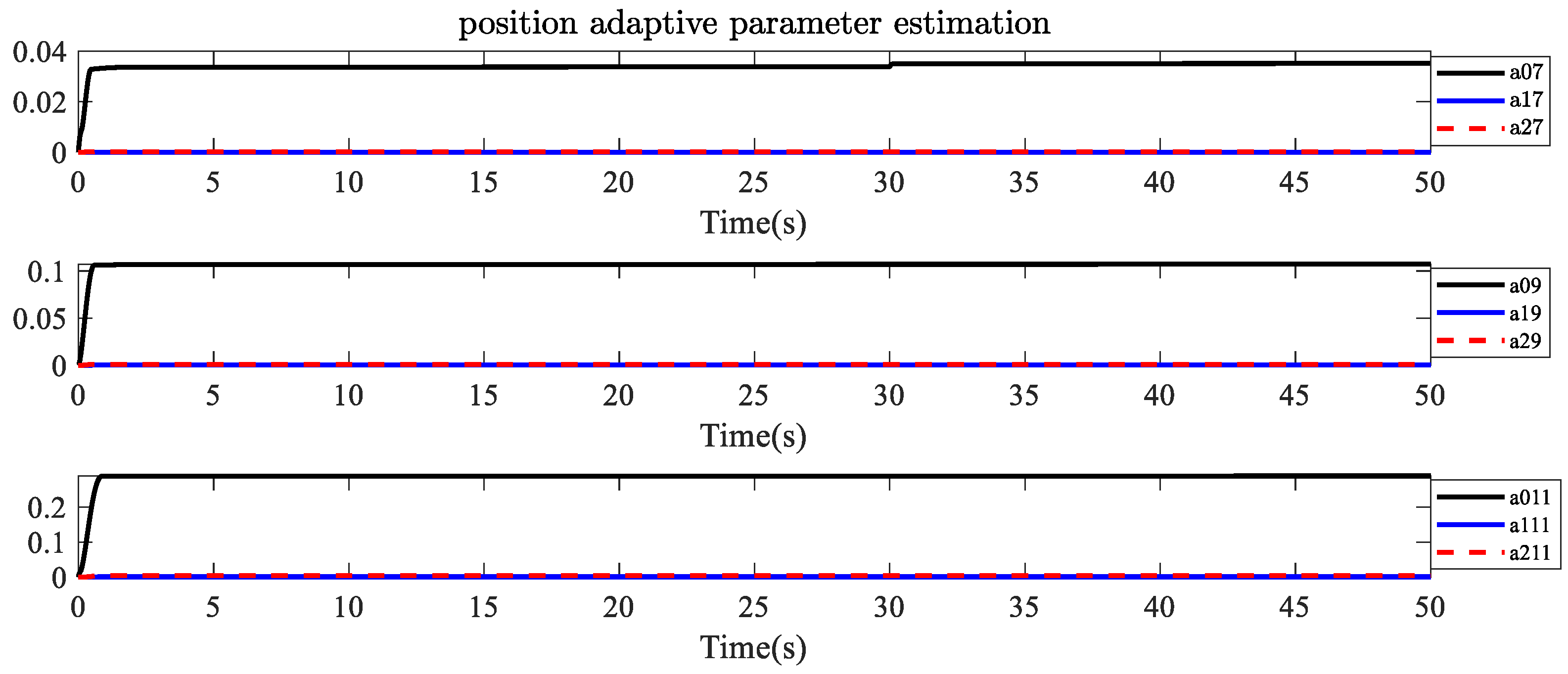
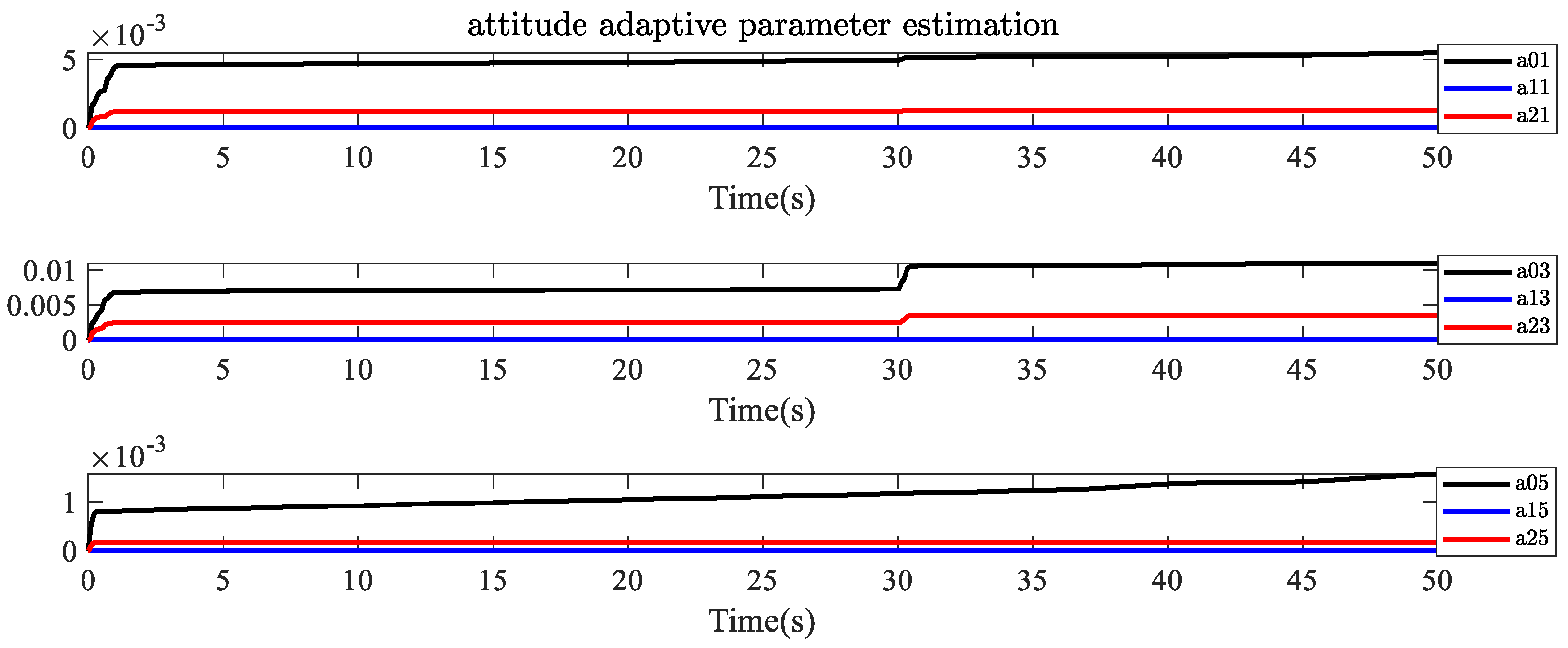
3.2.2. Adaptive Algorithm Design

An adaptive algorithm is developed to estimate the unknown upper bound of lumped disturbances. ${\hat{a}}_{0i}$, ${\hat{a}}_{1i}$, and ${\hat{a}}_{2i}$ are the estimate values of $a_{0i}$, $a_{1i}$, and $a_{2i}$. ${\tilde{a}}_{0i}=a_{0i}-{\hat{a}}_{0i}$, ${\tilde{a}}_{1i}=a_{1i}-{\hat{a}}_{1i}$, and ${\tilde{a}}_{2i}=a_{2i}-{\hat{a}}_{2i}$ are defined as the adaptive parameter estimation errors. In order to estimate the upper bound of lumped uncertainty online in real time, the adaptive law is designed as follows:

Adaptive law of rotation subsystem:

$$\begin{array}{c}{\dot{\widehat{a}}}_{01}={\mu }_{01}\left|s_1\right|{\left|e_2\right|}^{{\beta }_1-1},{\dot{\widehat{a}}}_{03}={\mu }_{03}\left|s_3\right|{\left|e_4\right|}^{{\beta }_3-1},{\dot{\widehat{a}}}_{05}={\mu }_{05}\left|s_5\right|{\left|e_6\right|}^{{\beta }_5-1}\hfill \\ {\dot{\widehat{a}}}_{11}={\mu }_{11}\left|s_1\right|\left|e_1\right|{\left|e_2\right|}^{{\beta }_1-1},{\dot{\widehat{a}}}_{13}={\mu }_{13}\left|s_3\right|\left|e_3\right|{\left|e_4\right|}^{{\beta }_3-1},{\dot{\widehat{a}}}_{15}={\mu }_{15}\left|s_5\right|\left|e_5\right|{\left|e_6\right|}^{{\beta }_5-1}\hfill \\ {\dot{\widehat{a}}}_{21}={\mu }_{21}\left|s_1\right|{\left|e_2\right|}^{{\beta }_1},{\dot{\widehat{a}}}_{23}={\mu }_{23}\left|s_3\right|{\left|e_4\right|}^{{\beta }_3},{\dot{\widehat{a}}}_{25}={\mu }_{25}\left|s_5\right|{\left|e_6\right|}^{{\beta }_5}\hfill \end{array}$$

(25)

Adaptive law of translation subsystem:

$$\begin{array}{l}{\dot{\widehat{a}}}_{07}={\mu }_{07}\left|s_7\right|{\left|e_8\right|}^{{\beta }_7-1},{\dot{\widehat{a}}}_{09}={\mu }_{09}\left|s_9\right|{\left|e_{10}\right|}^{{\beta }_9-1},{\dot{\widehat{a}}}_{011}={\mu }_{011}\left|s_{11}\right|{\left|e_{12}\right|}^{{\beta }_{11}-1}\hfill \\ {\dot{\widehat{a}}}_{17}={\mu }_{17}\left|s_7\right|\left|e_7\right|{\left|e_8\right|}^{{\beta }_7-1},{\dot{\widehat{a}}}_{19}={\mu }_{19}\left|s_9\right|\left|e_9\right|{\left|e_{10}\right|}^{{\beta }_9-1},{\dot{\widehat{a}}}_{111}={\mu }_{111}\left|s_{11}\right|\left|e_{11}\right|{\left|e_{12}\right|}^{{\beta }_{11}-1}\hfill \\ {\dot{\widehat{a}}}_{27}={\mu }_{27}\left|s_7\right|{\left|e_8\right|}^{{\beta }_7},{\dot{\widehat{a}}}_{29}={\mu }_{29}\left|s_9\right|{\left|e_{10}\right|}^{{\beta }_9},{\dot{\widehat{a}}}_{211}={\mu }_{211}\left|s_{11}\right|{\left|e_{12}\right|}^{{\beta }_{11}}\hfill \end{array}$$

(26)

where ${\mu }_{0i}$, ${\mu }_{1i}$, and ${\mu }_{2i}$$\left(i=1,3,5,\cdots ,11\right)$ are positive constants.

During the actual voyage of the vehicle, due to the influence of measurement noises, environmental disturbances, and parameter perturbations, the system state is usually not strictly fixed on the sliding-mode plane, so the adaptive parameter may increase infinitely, leading to system divergence. An easy way to overcome this shortcoming is to improve the adaptive law by using the dead zone technique, as follows [36]:

$${\dot{\widehat{a}}}_{0i}=\{\begin{array}{c}\hfill {\mu }_{0i}\left|s_i\right|{\left|e_{i+1}\right|}^{{\beta }_i-1},\left|s_i\right|>\epsilon \\ \hfill 0,\left|s_i\right|\le \epsilon \end{array},{\dot{\widehat{a}}}_{1i}=\{\begin{array}{c}\hfill {\mu }_{1i}\left|s_i\right|\left|e_i\right|{\left|e_{i+1}\right|}^{{\beta }_i-1},\left|s_i\right|>\epsilon \\ \hfill 0,\left|s_i\right|\le \epsilon \end{array},{\dot{\widehat{a}}}_{2i}=\{\begin{array}{c}\hfill {\mu }_{2i}\left|s_i\right|{\left|e_{i+1}\right|}^{{\beta }_i},\left|s_i\right|>\epsilon \\ \hfill 0,\left|s_i\right|\le \epsilon \end{array}$$

(27)

Lemma 1 

([37,38]). Consider a system (28a) if the Lyapunov function selected for its system state satisfies the following inequality (28b):

$$\dot{\xi }=f(\xi ),f(0)=0,\xi (0)={\xi }_0,\xi \in {ℝ}^n$$

(28a)

$$\dot{V}\left(\xi \right)\le -\kappa V^{\gamma }\left(\xi \right)$$

(28b)

where $f(\xi )={\left[f_1(\xi ),f_2(\xi ),\cdots ,f_n(\xi )\right]}^{\mathrm{T}}$ is a continuous vector field. $\kappa$ is the positive constant, $0<\gamma <1$, and $\xi$ is the state of the system. The system can be considered finite-time stable. Further, we can calculate the convergence time of $V\left(\xi \right)$ from the initial value $V\left(0\right)$ to be 0, and the settling time of the system is determined as follows:

$$t=\frac{V^{1-\gamma }\left(0\right)}{\kappa \left(1-\gamma \right)}$$

(29)

3.3. Proof of Stability

Theorem 1. 

For the translation subsystem (14a) and the nonsingular fast terminal sliding-mode surface (19a) under consideration, if the controller and the adaptive law of the translation system are selected as (24a) and (26), respectively, the system converges to the sliding-mode surface in a finite time, and, finally, the tracking errors of the outer loop converge to zero in a finite time.

Proof of Theorem 1. 

In order to prove Theorem 1, the following Lyapunov function is selected for the translation subsystem:

$$V_P=\frac{1}{2}{\mathit{S}}_p^{\mathrm{T}}{\mathit{S}}_p+{\displaystyle \sum _{i=0}^2\frac{{\gamma }_{i7}{\beta }_7{b}_8}{2{\mu }_{i7}}}{\tilde{a}}_{i7}^2+{\displaystyle \sum _{i=0}^2\frac{{\gamma }_{i9}{\beta }_9{b}_{10}}{2{\mu }_{i9}}}{\tilde{a}}_{i9}^2+{\displaystyle \sum _{i=0}^2\frac{{\gamma }_{i11}{\beta }_{11}{b}_{12}}{2{\mu }_{i11}}}{\tilde{a}}_{i11}^2$$

(30)

where ${\gamma }_{i7}$, ${\gamma }_{i9}$, ${\gamma }_{i11}>1 (i=0,1,2)$ are positive constants.

By taking the time derivative of Equation (30) and substituting the controller Equation (24a) into the time derivative of $V_P$, we can obtain

$$\begin{array}{cc}\hfill {\dot{V}}_P& =s_7{\dot{s}}_7+s_9{\dot{s}}_9+s_{11}{\dot{s}}_{11}-{\displaystyle \sum _{i=0}^2\frac{{\gamma }_{i7}{\beta }_7{b}_8}{{\mu }_{i7}}}{\tilde{a}}_{i7}{\dot{\widehat{a}}}_{i7}-{\displaystyle \sum _{i=0}^2\frac{{\gamma }_{i9}{\beta }_9{b}_{10}}{{\mu }_{i9}}}{\tilde{a}}_{i9}{\dot{\widehat{a}}}_{i9}-{\displaystyle \sum _{i=0}^2\frac{{\gamma }_{i11}{\beta }_{11}{b}_{12}}{{\mu }_{i11}}}{\tilde{a}}_{i11}{\dot{\widehat{a}}}_{i11}\hfill \\ & =s_7{\beta }_7{b}_8{\left|e_8\right|}^{{\beta }_7-1}\left(-c_7{s}_7-K_{7}sign\left(s_7\right)sign\left(s_7\right)+d_x\right)\hfill \\ & +s_9{\beta }_9{b}_{10}{\left|e_{10}\right|}^{{\beta }_9-1}\left(-c_9{s}_9-K_{9}sign\left(s_9\right)+d_y\right)\hfill \\ & +s_{11}{\beta }_{11}{b}_{12}{\left|e_{12}\right|}^{{\beta }_{11}-1}\left(-c_{11}{s}_{11}-K_{11}sign\left(s_{11}\right)+d_z\right)\hfill \\ & -{\displaystyle \sum _{i=0}^2\frac{{\gamma }_{i7}{\beta }_7{b}_8}{{\mu }_{i7}}}{\tilde{a}}_{i7}{\dot{\widehat{a}}}_{i7}-{\displaystyle \sum _{i=0}^2\frac{{\gamma }_{i9}{\beta }_9{b}_{10}}{{\mu }_{i9}}}{\tilde{a}}_{i9}{\dot{\widehat{a}}}_{i9}-{\displaystyle \sum _{i=0}^2\frac{{\gamma }_{i11}{\beta }_{11}{b}_{12}}{{\mu }_{i11}}}{\tilde{a}}_{i11}{\dot{\widehat{a}}}_{i11}\hfill \\ & =s_7{\beta }_7{b}_8{\left|e_8\right|}^{{\beta }_7-1}\left(-c_7{s}_7-\left({\widehat{a}}_{07}+{\widehat{a}}_{17}\left|e_7\right|+{\widehat{a}}_{27}\left|e_8\right|+{\delta }_7\right)sign\left(s_7\right)+d_x\right)\hfill \\ & +s_9{\beta }_9{b}_{10}{\left|e_{10}\right|}^{{\beta }_9-1}\left(-c_9{s}_9-\left({\widehat{a}}_{09}+{\widehat{a}}_{19}\left|e_9\right|+{\widehat{a}}_{29}\left|e_{10}\right|+{\delta }_9\right)sign\left(s_9\right)+d_y\right)\hfill \\ & +s_{11}{\beta }_{11}{b}_{12}{\left|e_{12}\right|}^{{\beta }_{11}-1}\left(-c_{11}{s}_{11}-\left({\widehat{a}}_{011}+{\widehat{a}}_{111}\left|e_{11}\right|+{\widehat{a}}_{211}\left|e_{12}\right|+{\delta }_{11}\right)sign\left(s_{11}\right)+d_z\right)\hfill \\ & -{\displaystyle \sum _{i=0}^2\frac{{\gamma }_{i7}{\beta }_7{b}_8}{{\mu }_{i7}}}{\tilde{a}}_{i7}{\dot{\widehat{a}}}_{i7}-{\displaystyle \sum _{i=0}^2\frac{{\gamma }_{i9}{\beta }_9{b}_{10}}{{\mu }_{i9}}}{\tilde{a}}_{i9}{\dot{\widehat{a}}}_{i9}-{\displaystyle \sum _{i=0}^2\frac{{\gamma }_{i11}{\beta }_{11}{b}_{12}}{{\mu }_{i11}}}{\tilde{a}}_{i11}{\dot{\widehat{a}}}_{i11}\hfill \\ & \le {\beta }_7{b}_8{\left|e_8\right|}^{{\beta }_7-1}\left(-c_7{s}_7^2-{\delta }_7\left|s_7\right|\right)+{\beta }_9{b}_{10}{\left|e_{10}\right|}^{{\beta }_9-1}\left(-c_9{s}_9^2-{\delta }_9\left|s_9\right|\right)+{\beta }_{11}{b}_{12}{\left|e_{12}\right|}^{{\beta }_{11}-1}\left(-c_9{s}_{11}^2-{\delta }_{11}\left|s_{11}\right|\right)\hfill \\ & +{\beta }_7{b}_8{\left|e_8\right|}^{{\beta }_7-1}\left|s_7\right|\left({\tilde{a}}_{07}+{\tilde{a}}_{17}\left|e_7\right|+{\tilde{a}}_{27}\left|e_8\right|+{\delta }_7\right)+{\beta }_9{b}_{10}{\left|e_{10}\right|}^{{\beta }_9-1}\left|s_9\right|\left({\tilde{a}}_{09}+{\tilde{a}}_{19}\left|e_9\right|+{\tilde{a}}_{29}\left|e_{10}\right|+{\delta }_9\right)\hfill \\ & +{\beta }_{11}{b}_{12}{\left|e_{12}\right|}^{{\beta }_{11}-1}\left|s_{11}\right|\left({\tilde{a}}_{011}+{\tilde{a}}_{111}\left|e_{11}\right|+{\tilde{a}}_{211}\left|e_{12}\right|+{\delta }_{11}\right)\hfill \\ & -{\displaystyle \sum _{i=0}^2\frac{{\gamma }_{i7}{\beta }_7{b}_8}{{\mu }_{i7}}}{\tilde{a}}_{i7}{\dot{\widehat{a}}}_{i7}-{\displaystyle \sum _{i=0}^2\frac{{\gamma }_{i9}{\beta }_9{b}_{10}}{{\mu }_{i9}}}{\tilde{a}}_{i9}{\dot{\widehat{a}}}_{i9}-{\displaystyle \sum _{i=0}^2\frac{{\gamma }_{i11}{\beta }_{11}{b}_{12}}{{\mu }_{i11}}}{\tilde{a}}_{i11}{\dot{\widehat{a}}}_{i11}\hfill \end{array}$$

(31)

Substituting the adaptive law (26) into Equation (31), yields

$$\begin{array}{cc}\hfill {\dot{V}}_P& \le {\beta }_7{b}_8{\left|e_8\right|}^{{\beta }_7-1}\left(-c_7{s}_7^2-{\delta }_7\left|s_7\right|\right)+{\beta }_9{b}_{10}{\left|e_{10}\right|}^{{\beta }_9-1}\left(-c_9{s}_9^2-{\delta }_9\left|s_9\right|\right)+{\beta }_{11}{b}_{12}{\left|e_{12}\right|}^{{\beta }_{11}-1}\left(-c_9{s}_{11}^2-{\delta }_{11}\left|s_{11}\right|\right)\hfill \\ & +{\beta }_7{b}_8\left|s_7\right|{\left|e_8\right|}^{{\beta }_7-1}\left({\tilde{a}}_{07}+{\tilde{a}}_{17}\left|e_7\right|+{\tilde{a}}_{27}\left|e_8\right|\right)+{\beta }_9{b}_{10}\left|s_9\right|{\left|e_{10}\right|}^{{\beta }_9-1}\left({\tilde{a}}_{09}+{\tilde{a}}_{19}\left|e_9\right|+{\tilde{a}}_{29}\left|e_{10}\right|\right)\hfill \\ & +{\beta }_{11}{b}_{12}\left|s_{11}\right|{\left|e_{12}\right|}^{{\beta }_{11}-1}\left({\tilde{a}}_{011}+{\tilde{a}}_{111}\left|e_{11}\right|+{\tilde{a}}_{211}\left|e_{12}\right|\right)-{\gamma }_{i7}{\beta }_7{b}_8\left|s_7\right|{\left|e_8\right|}^{{\beta }_7-1}\left({\tilde{a}}_{07}+{\tilde{a}}_{17}\left|e_7\right|+{\tilde{a}}_{27}\left|e_8\right|\right)\hfill \\ & -{\gamma }_{i9}{\beta }_9{b}_{10}\left|s_9\right|{\left|e_{10}\right|}^{{\beta }_9-1}\left({\tilde{a}}_{09}+{\tilde{a}}_{19}\left|e_9\right|+{\tilde{a}}_{29}\left|e_{10}\right|\right)-{\gamma }_{i11}{\beta }_{11}{b}_{12}\left|s_{11}\right|{\left|e_{12}\right|}^{{\beta }_{11}-1}\left({\tilde{a}}_{011}+{\tilde{a}}_{111}\left|e_{11}\right|+{\tilde{a}}_{211}\left|e_{12}\right|\right)\hfill \\ & \le -{\beta }_7{b}_8{\left|e_8\right|}^{{\beta }_7-1}{\delta }_7\left|s_7\right|-{\beta }_9{b}_{10}{\left|e_{10}\right|}^{{\beta }_9-1}{\delta }_9\left|s_9\right|-{\beta }_{11}{b}_{12}{\left|e_{12}\right|}^{{\beta }_{11}-1}{\delta }_{11}\left|s_{11}\right|-\left({\gamma }_{i7}-1\right){\beta }_7{b}_8{\left|e_8\right|}^{{\beta }_7-1}\left|s_7\right|\left({\tilde{a}}_{07}+{\tilde{a}}_{17}\left|e_7\right|+{\tilde{a}}_{27}\left|e_8\right|\right)\hfill \\ & -\left({\gamma }_{i9}-1\right){\beta }_9{b}_{10}\left|s_9\right|{\left|e_{10}\right|}^{{\beta }_9-1}\left({\tilde{a}}_{09}+{\tilde{a}}_{19}\left|e_9\right|+{\tilde{a}}_{29}\left|e_{10}\right|\right)-\left({\gamma }_{i11}-1\right){\beta }_{11}{b}_{12}\left|s_{11}\right|{\left|e_{12}\right|}^{{\beta }_{11}-1}\left({\tilde{a}}_{011}+{\tilde{a}}_{111}\left|e_{11}\right|+{\tilde{a}}_{211}\left|e_{12}\right|\right)\hfill \end{array}$$

(32)

To simplify the above expression, the following variables are defined:

$$\begin{array}{cc}\hfill {\rho }_7& ={\delta }_7{\beta }_7{b}_8{\left|e_8\right|}^{{\beta }_7-1},{\rho }_9={\delta }_9{\beta }_9{b}_{10}{\left|e_{10}\right|}^{{\beta }_9-1},{\rho }_{11}={\delta }_{11}{\beta }_{11}{b}_{12}{\left|e_{12}\right|}^{{\beta }_{11}-1}\hfill \\ \hfill {\rho }_{07}& =\left({\gamma }_{07}-1\right){\beta }_7{b}_8{\left|e_8\right|}^{{\beta }_7-1}\left|s_7\right|,{\rho }_{17}=\left({\gamma }_{17}-1\right){\beta }_7{b}_8\left|e_7\right|{\left|e_8\right|}^{{\beta }_7-1}\left|s_7\right|,{\rho }_{27}=\left({\gamma }_{27}-1\right){\beta }_7{b}_8{\left|e_8\right|}^{{\beta }_7}\left|s_7\right|\hfill \\ \hfill {\rho }_{09}& =\left({\gamma }_{09}-1\right){\beta }_9{b}_{10}{\left|e_{10}\right|}^{{\beta }_9-1}\left|s_9\right|,{\rho }_{19}=\left({\gamma }_{19}-1\right){\beta }_9{b}_{10}\left|e_9\right|{\left|e_{10}\right|}^{{\beta }_9-1}\left|s_9\right|,{\rho }_{29}=\left({\gamma }_{29}-1\right){\beta }_9{b}_{10}{\left|e_{10}\right|}^{{\beta }_9}\left|s_9\right|\hfill \\ \hfill {\rho }_{011}& =\left({\gamma }_{011}-1\right){\beta }_{11}{b}_{12}{\left|e_{12}\right|}^{{\beta }_{11}-1}\left|s_{11}\right|,{\rho }_{111}=\left({\gamma }_{111}-1\right){\beta }_{11}{b}_{12}\left|e_{11}\right|{\left|e_{12}\right|}^{{\beta }_{11}-1}\left|s_{11}\right|,{\rho }_{211}=\left({\gamma }_{211}-1\right){\beta }_{11}{b}_{12}{\left|e_{12}\right|}^{{\beta }_{11}}\left|s_{11}\right|\hfill \end{array}$$

(33)

We can then obtain the following inequality:

$$\begin{array}{cc}\hfill {\dot{V}}_P& \le -{\rho }_7\left|s_7\right|-{\rho }_9\left|s_9\right|-{\rho }_{11}\left|s_{11}\right|-{\displaystyle \sum _{i=0}^2{\rho }_{i7}\left|{\tilde{a}}_{i7}\right|}-{\displaystyle \sum _{i=0}^2{\rho }_{i9}\left|{\tilde{a}}_{i9}\right|}-{\displaystyle \sum _{i=0}^2{\rho }_{i11}\left|{\tilde{a}}_{i11}\right|}\hfill \\ & \le -\sqrt{2}{\rho }_7{\left(\frac{1}{2}{s}_7^2\right)}^{1/2}-\sqrt{2}{\rho }_9{\left(\frac{1}{2}{s}_9^2\right)}^{1/2}-\sqrt{2}{\rho }_{11}{\left(\frac{1}{2}{s}_{11}^2\right)}^{1/2}-\sqrt{2{\mu }_{i7}/{\gamma }_{i7}{\beta }_7{b}_8}{\rho }_{i7}{\left({\displaystyle \sum _{i=0}^2\frac{{\gamma }_{i7}{\beta }_7{b}_8}{2{\mu }_{i7}}}{\tilde{a}}_{i7}^2\right)}^{1/2}\hfill \\ & -\sqrt{2{\mu }_{i9}/{\gamma }_{i9}{\beta }_9{b}_{10}}{\rho }_{i9}{\left({\displaystyle \sum _{i=0}^2\frac{{\gamma }_{i9}{\beta }_9{b}_{10}}{2{\mu }_{i9}}}{\tilde{a}}_{i9}^2\right)}^{1/2}-\sqrt{2{\mu }_{i11}/{\gamma }_{i11}{\beta }_{11}{b}_{12}}{\rho }_{i11}{\left({\displaystyle \sum _{i=0}^2\frac{{\gamma }_{i11}{\beta }_{11}{b}_{12}}{2{\mu }_{i11}}}{\tilde{a}}_{i11}^2\right)}^{{}^{1/2}}\hfill \\ & \le {\rho }_P{V}_P^{1/2}\hfill \end{array}$$

(34)

where ${\rho }_{\Theta }=\mathit{min}\{\sqrt{2}{\rho }_1,\sqrt{2}{\rho }_3,\sqrt{2}{\rho }_5,\sqrt{2{\mu }_{i1}/{\gamma }_{i1}{\beta }_1{b}_2}{\rho }_{i1},\sqrt{2{\mu }_{i3}/{\gamma }_{i3}{\beta }_3{b}_4}{\rho }_{i3},\sqrt{2{\mu }_{i5}/{\gamma }_{i5}{\beta }_5{b}_6}{\rho }_{i5}\}$. □

In this part, a translation subsystem controller based on the ANFTSMC algorithm is designed. It can be seen from the above Lyapunov analysis that the finite-time stability of the outer ring can be guaranteed. Similarly, the finite-time stability of the attitude loop is proven in the following sections.

Theorem 2. 

Considering the coaxial HAUV’s rotation subsystem (14b), if the controller and adaptive law are designed as Equations (24b) and (25), attitude tracking errors converge to zero in a finite time.

Proof. 

Next, the Lyapunov function of the rotation subsystem is determined as shown below:

$$\begin{array}{cc}\hfill V_A& =\frac{1}{2}{\mathit{S}}_A^{\mathrm{T}}{\mathit{S}}_A+{\displaystyle \sum _{i=0}^2\frac{{\gamma }_{i1}{\beta }_1{b}_2}{2{\mu }_{i1}}}{\tilde{a}}_{i1}^2+{\displaystyle \sum _{i=0}^2\frac{{\gamma }_{i3}{\beta }_3{b}_4}{2{\mu }_{i3}}}{\tilde{a}}_{i3}^2+{\displaystyle \sum _{i=0}^2\frac{{\gamma }_{i5}{\beta }_5{b}_6}{2{\mu }_{i5}}}{\tilde{a}}_{i5}^2\hfill \\ & =\frac{1}{2}{s}_1^2+\frac{1}{2}{s}_3^2+\frac{1}{2}{s}_5^2+{\displaystyle \sum _{i=0}^2\frac{{\gamma }_{i1}{\beta }_1{b}_2}{2{\mu }_{i1}}}{\tilde{a}}_{i1}^2+{\displaystyle \sum _{i=0}^2\frac{{\gamma }_{i3}{\beta }_3{b}_4}{2{\mu }_{i3}}}{\tilde{a}}_{i3}^2+{\displaystyle \sum _{i=0}^2\frac{{\gamma }_{i5}{\beta }_5{b}_6}{2{\mu }_{i5}}}{\tilde{a}}_{i5}^2\hfill \end{array}$$

(35)

By calculating the derivative of Equation (35) and substituting the controller Equation (24b) of the rotation subsystem, we can obtain the following:

$$\begin{array}{cc}\hfill {\dot{V}}_A& =s_1{\dot{s}}_1+s_3{\dot{s}}_3+s_5{\dot{s}}_5-{\displaystyle \sum _{i=0}^2\frac{{\gamma }_{i1}{\beta }_1{b}_2}{{\mu }_{i1}}}{\tilde{a}}_{i1}{\dot{\widehat{a}}}_{i1}-{\displaystyle \sum _{i=0}^2\frac{{\gamma }_{i3}{\beta }_3{b}_4}{{\mu }_{i3}}}{\tilde{a}}_{i3}{\dot{\widehat{a}}}_{i3}-{\displaystyle \sum _{i=0}^2\frac{{\gamma }_{i5}{\beta }_5{b}_6}{{\mu }_{i5}}}{\tilde{a}}_{i5}{\dot{\widehat{a}}}_{i5}\hfill \\ & =s_1{\beta }_1{b}_2{\left|e_2\right|}^{{\beta }_1-1}\left(-c_1{s}_1-\left({\widehat{a}}_{01}+{\widehat{a}}_{11}\left|e_1\right|+{\widehat{a}}_{21}\left|e_2\right|+{\delta }_1\right)sign\left(s_1\right)+d_{\varphi }\right)\hfill \\ & +s_3{\beta }_3{b}_4{\left|e_4\right|}^{{\beta }_3-1}\left(-c_3{s}_3-\left({\widehat{a}}_{03}+{\widehat{a}}_{13}\left|e_3\right|+{\widehat{a}}_{23}\left|e_4\right|+{\delta }_3\right)sign\left(s_3\right)+d_{\theta }\right)\hfill \\ & +s_5{\beta }_5{b}_6{\left|e_6\right|}^{{\beta }_5-1}\left(-c_5{s}_5-\left({\widehat{a}}_{05}+{\widehat{a}}_{15}\left|e_5\right|+{\widehat{a}}_{25}\left|e_6\right|+{\delta }_5\right)sign\left(s_5\right)+d_{\psi }\right)\hfill \\ & -{\displaystyle \sum _{i=0}^2\frac{{\gamma }_{i1}{\beta }_1{b}_2}{{\mu }_{i1}}}{\tilde{a}}_{i1}{\dot{\widehat{a}}}_{i1}-{\displaystyle \sum _{i=0}^2\frac{{\gamma }_{i3}{\beta }_3{b}_4}{{\mu }_{i3}}}{\tilde{a}}_{i3}{\dot{\widehat{a}}}_{i3}-{\displaystyle \sum _{i=0}^2\frac{{\gamma }_{i5}{\beta }_5{b}_6}{{\mu }_{i5}}}{\tilde{a}}_{i5}{\dot{\widehat{a}}}_{i5}\hfill \\ & \le {\beta }_1{b}_2{\left|e_2\right|}^{{\beta }_1-1}\left(-c_1{s}_1^2-{\delta }_1\left|s_1\right|\right)+{\beta }_3{b}_4{\left|e_4\right|}^{{\beta }_3-1}\left(-c_3{s}_3^2-{\delta }_3\left|s_3\right|\right)+{\beta }_5{b}_6{\left|e_6\right|}^{{\beta }_5-1}\left(-c_5{s}_5^2-{\delta }_5\left|s_5\right|\right)\hfill \\ & +{\beta }_1{b}_2{\left|e_2\right|}^{{\beta }_1-1}\left|s_1\right|\left({\tilde{a}}_{01}+{\tilde{a}}_{11}\left|e_1\right|+{\tilde{a}}_{21}\left|e_2\right|+{\delta }_1\right)+{\beta }_3{b}_4{\left|e_4\right|}^{{\beta }_3-1}\left|s_3\right|\left({\tilde{a}}_{03}+{\tilde{a}}_{13}\left|e_3\right|+{\tilde{a}}_{23}\left|e_4\right|+{\delta }_3\right)\hfill \\ & +{\beta }_5{b}_6{\left|e_6\right|}^{{\beta }_5-1}\left|s_5\right|\left({\tilde{a}}_{05}+{\tilde{a}}_{15}\left|e_5\right|+{\tilde{a}}_{25}\left|e_6\right|+{\delta }_5\right)-{\displaystyle \sum _{i=0}^2\frac{{\gamma }_{i1}{\beta }_1{b}_2}{{\mu }_{i1}}}{\tilde{a}}_{i1}{\dot{\widehat{a}}}_{i1}-{\displaystyle \sum _{i=0}^2\frac{{\gamma }_{i3}{\beta }_3{b}_4}{{\mu }_{i3}}}{\tilde{a}}_{i3}{\dot{\widehat{a}}}_{i3}-{\displaystyle \sum _{i=0}^2\frac{{\gamma }_{i5}{\beta }_5{b}_6}{{\mu }_{i5}}}{\tilde{a}}_{i5}{\dot{\widehat{a}}}_{i5}\hfill \end{array}$$

(36)

Considering the adaptive law (25), it can be obtained as follows:

$$\begin{array}{cc}\hfill {\dot{V}}_A& \le {\beta }_1{b}_2{\left|e_2\right|}^{{\beta }_1-1}\left(-c_1{s}_1^2-{\delta }_1\left|s_1\right|\right)+{\beta }_3{b}_4{\left|e_4\right|}^{{\beta }_3-1}\left(-c_3{s}_3^2-{\delta }_3\left|s_3\right|\right)+{\beta }_5{b}_6{\left|e_6\right|}^{{\beta }_5-1}\left(-c_5{s}_5^2-{\delta }_5\left|s_5\right|\right)\hfill \\ & +{\beta }_1{b}_2{\left|e_2\right|}^{{\beta }_1-1}\left|s_1\right|\left({\tilde{a}}_{01}+{\tilde{a}}_{11}\left|e_1\right|+{\tilde{a}}_{21}\left|e_2\right|\right)+{\beta }_3{b}_4{\left|e_4\right|}^{{\beta }_3-1}\left|s_3\right|\left({\tilde{a}}_{03}+{\tilde{a}}_{13}\left|e_3\right|+{\tilde{a}}_{23}\left|e_4\right|\right)\hfill \\ & +{\beta }_5{b}_6{\left|e_6\right|}^{{\beta }_5-1}\left|s_5\right|\left({\tilde{a}}_{05}+{\tilde{a}}_{15}\left|e_5\right|+{\tilde{a}}_{25}\left|e_6\right|\right)-{\gamma }_{i1}{\beta }_1{b}_2{\left|e_2\right|}^{{\beta }_1-1}\left|s_1\right|\left({\tilde{a}}_{01}+{\tilde{a}}_{11}\left|e_1\right|+{\tilde{a}}_{21}\left|e_2\right|\right)\hfill \\ & -{\gamma }_{i3}{\beta }_3{b}_4{\left|e_4\right|}^{{\beta }_3-1}\left|s_3\right|\left({\tilde{a}}_{03}+{\tilde{a}}_{13}\left|e_3\right|+{\tilde{a}}_{23}\left|e_4\right|\right)-{\gamma }_{i5}{\beta }_5{b}_6{\left|e_6\right|}^{{\beta }_5-1}\left|s_5\right|\left({\tilde{a}}_{05}+{\tilde{a}}_{15}\left|e_5\right|+{\tilde{a}}_{25}\left|e_6\right|\right)\hfill \\ & \le -{\delta }_1{\beta }_1{b}_2{\left|e_2\right|}^{{\beta }_1-1}\left|s_1\right|-{\delta }_3{\beta }_3{b}_4{\left|e_4\right|}^{{\beta }_3-1}\left|s_3\right|-{\delta }_5{\beta }_5{b}_6{\left|e_6\right|}^{{\beta }_5-1}\left|s_5\right|-\left({\gamma }_{i1}-1\right){\beta }_1{b}_2{\left|e_2\right|}^{{\beta }_1-1}\left|s_1\right|\left({\tilde{a}}_{01}+{\tilde{a}}_{11}\left|e_1\right|+{\tilde{a}}_{21}\left|e_2\right|\right)\hfill \\ & -\left({\gamma }_{i3}-1\right){\beta }_3{b}_4{\left|e_4\right|}^{{\beta }_3-1}\left|s_3\right|\left({\tilde{a}}_{03}+{\tilde{a}}_{13}\left|e_3\right|+{\tilde{a}}_{23}\left|e_4\right|\right)-\left({\gamma }_{i5}-1\right){\beta }_5{b}_6{\left|e_6\right|}^{{\beta }_5-1}\left|s_5\right|\left({\tilde{a}}_{05}+{\tilde{a}}_{15}\left|e_5\right|+{\tilde{a}}_{25}\left|e_6\right|\right)\hfill \end{array}$$

(37)

Similar to the proof process for the outer loop, we further simplify the representation inequality (37) as follows:

$${\dot{V}}_A\le -{\rho }_1\left|s_1\right|-{\rho }_3\left|s_3\right|-{\rho }_5\left|s_5\right|-{\displaystyle \sum _{i=0}^2{\rho }_{i1}\left|{\tilde{a}}_{i1}\right|}-{\displaystyle \sum _{i=0}^2{\rho }_{i3}\left|{\tilde{a}}_{i3}\right|}-{\displaystyle \sum _{i=0}^2{\rho }_{i5}\left|{\tilde{a}}_{i5}\right|}$$

(38)

where

$$\begin{array}{cc}\hfill {\rho }_1& ={\delta }_1{\beta }_1{b}_2{\left|e_2\right|}^{{\beta }_1-1},{\rho }_3={\delta }_3{\beta }_3{b}_4{\left|e_4\right|}^{{\beta }_3-1},{\rho }_5={\delta }_5{\beta }_5{b}_6{\left|e_6\right|}^{{\beta }_5-1}\hfill \\ \hfill {\rho }_{01}& =\left({\gamma }_{01}-1\right){\beta }_1{b}_2{\left|e_2\right|}^{{\beta }_1-1}\left|s_1\right|,{\rho }_{11}=\left({\gamma }_{11}-1\right){\beta }_1{b}_2\left|e_1\right|{\left|e_2\right|}^{{\beta }_1-1}\left|s_1\right|,{\rho }_{21}=\left({\gamma }_{21}-1\right){\beta }_1{b}_2{\left|e_2\right|}^{{\beta }_1}\left|s_1\right|\hfill \\ \hfill {\rho }_{03}& =\left({\gamma }_{03}-1\right){\beta }_3{b}_4{\left|e_4\right|}^{{\beta }_3-1}\left|s_3\right|,{\rho }_{13}=\left({\gamma }_{13}-1\right){\beta }_3{b}_4\left|e_3\right|{\left|e_4\right|}^{{\beta }_3-1}\left|s_3\right|,{\rho }_{23}=\left({\gamma }_{23}-1\right){\beta }_3{b}_4{\left|e_4\right|}^{{\beta }_3}\left|s_3\right|\hfill \\ \hfill {\rho }_{05}& =\left({\gamma }_{05}-1\right){\beta }_5{b}_6{\left|e_6\right|}^{{\beta }_5-1}\left|s_5\right|,{\rho }_{15}=\left({\gamma }_{15}-1\right){\beta }_5{b}_6\left|e_5\right|{\left|e_6\right|}^{{\beta }_5-1}\left|s_5\right|,{\rho }_{25}=\left({\gamma }_{25}-1\right){\beta }_5{b}_6{\left|e_6\right|}^{{\beta }_5}\left|s_5\right|\hfill \end{array}$$

(39)

By further simplifying Equation (39), we can obtain

$$\begin{array}{cc}\hfill {\dot{V}}_A& \le -\sqrt{2}{\rho }_1{\left(\frac{1}{2}{s}_1^2\right)}^{1/2}-\sqrt{2}{\rho }_3{\left(\frac{1}{2}{s}_3^2\right)}^{1/2}-\sqrt{2}{\rho }_5{\left(\frac{1}{2}{s}_5^2\right)}^{1/2}-\sqrt{2{\mu }_{i1}/{\gamma }_{i1}{\beta }_1{b}_2}{\rho }_{i1}{\left({\displaystyle \sum _{i=0}^2\frac{{\gamma }_{i1}{\beta }_1{b}_2}{2{\mu }_{i1}}}{\tilde{a}}_{i1}^2\right)}^{1/2}\hfill \\ & -\sqrt{2{\mu }_{i3}/{\gamma }_{i3}{\beta }_3{b}_4}{\rho }_{i3}{\left({\displaystyle \sum _{i=0}^2\frac{{\gamma }_{i3}{\beta }_3{b}_4}{2{\mu }_{i3}}}{\tilde{a}}_{i3}^2\right)}^{1/2}-\sqrt{2{\mu }_{i5}/{\gamma }_{i5}{\beta }_5{b}_6}{\rho }_{i5}{\left({\displaystyle \sum _{i=0}^2\frac{{\gamma }_{i5}{\beta }_5{b}_6}{2{\mu }_{i5}}}{\tilde{a}}_{i5}^2\right)}^{{}^{1/2}}\hfill \\ & \le {\rho }_{\Theta }{V}_A^{1/2}\hfill \end{array}$$

(40)

where ${\rho }_{\Theta }=min\left\{\sqrt{2}{\rho }_1,\sqrt{2}{\rho }_3,\sqrt{2}{\rho }_5,\sqrt{2{\mu }_{i1}/{\gamma }_{i1}{\beta }_1{b}_2}{\rho }_{i1},\sqrt{2{\mu }_{i3}/{\gamma }_{i3}{\beta }_3{b}_4}{\rho }_{i3},\sqrt{2{\mu }_{i5}/{\gamma }_{i5}{\beta }_5{b}_6}{\rho }_{i5}\right\}$. □

It can be seen from the above analysis that the finite-time stability of the attitude ring is guaranteed according to Lemma 1.

In order to prove the global closed-loop stability of the system, the Lyapunov functions of the coaxial HAUV system are determined using the following equation:

$$V=V_P+V_A$$

(41)

According to the proof process of Theorems 1 and 2 above, it can be obtained as follows:

$$\dot{V}={\dot{V}}_P+{\dot{V}}_A\le -{\rho }_P{V}_P^{1/2}-{\rho }_{\Theta }{V}_R^{1/2}\le -\rho V^{1/2}$$

(42)

where $\rho =min\left\{{\rho }_{\Theta },{\rho }_P\right\}$.□

Finally, the global finite-time stability of rotation and shift-tracking errors is proven using the Lyapunov method. The above proof process is complete.

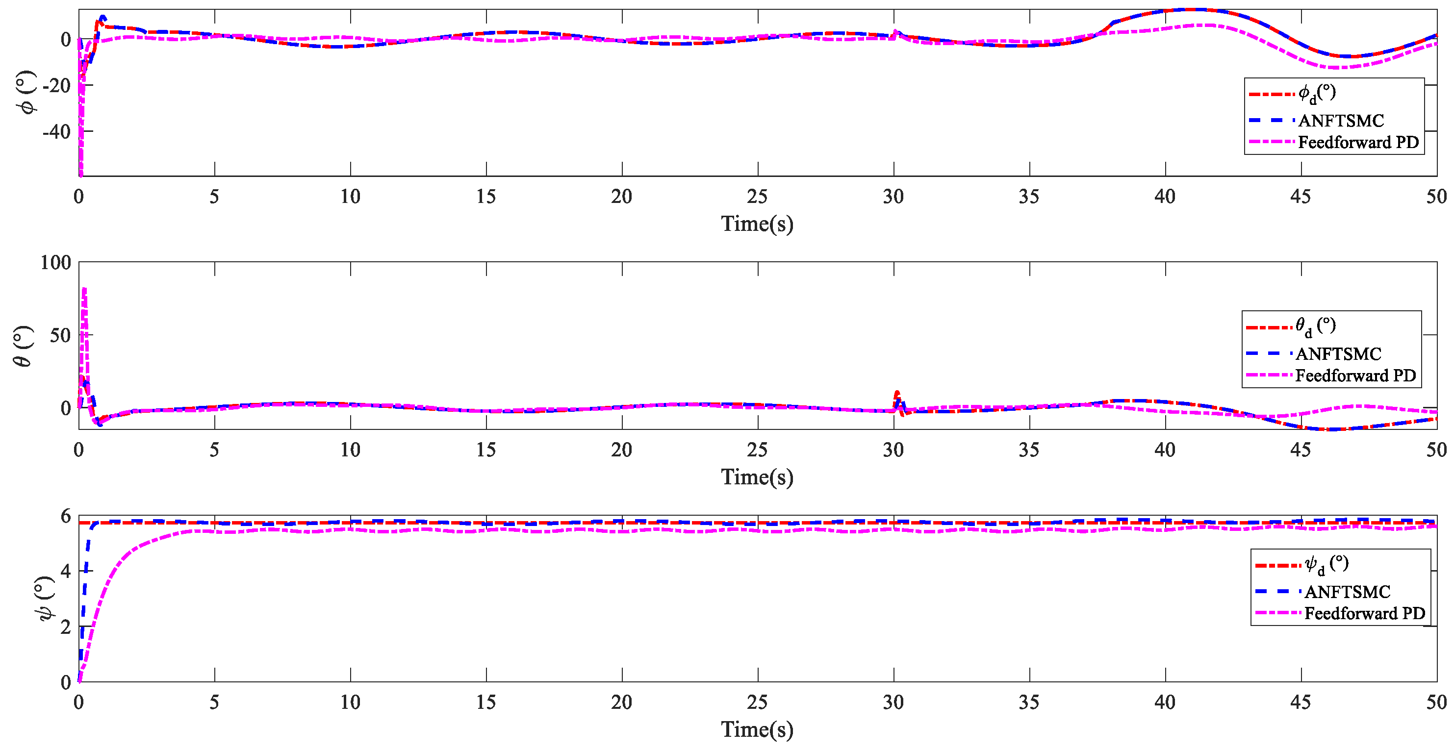
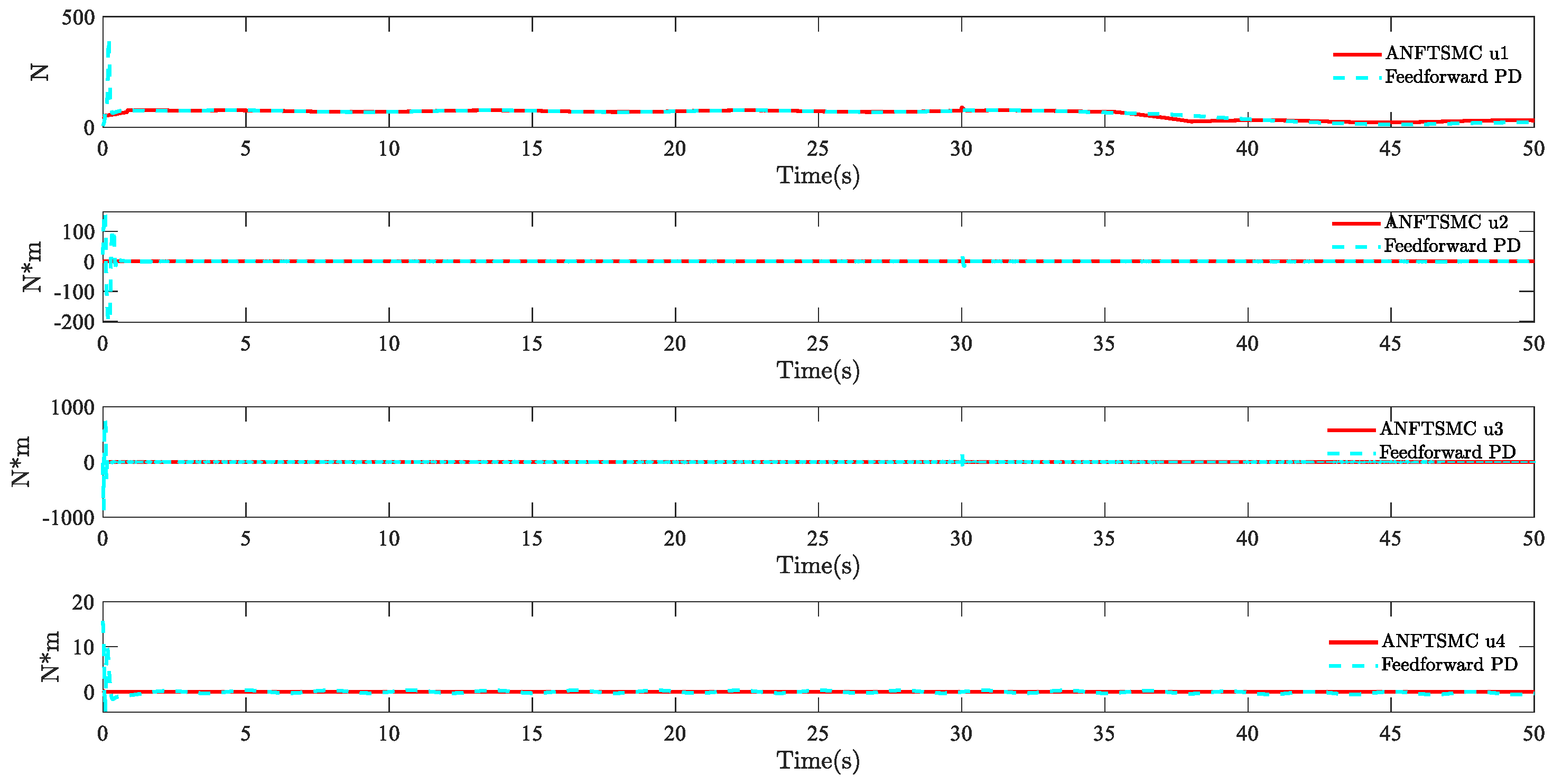
4. Simulation and Discussion

Based on the above theoretical analysis, we have verified the effectiveness of the designed ANFTSMC algorithm in coaxial HAUV control at the theoretical level. The main purpose of this section is to verify the effectiveness of the designed controller through simulation. Next, we conducted a simulation of HAUV motion control via Simulink and selected the two most typical working conditions (water-exit and water-entry).

To verify the effectiveness of the ANFTSNC controller designed for the coaxial HAUV, we developed a simple feedforward PD controller as a reference comparison item. The feedforward PD controller is designed as follows:

$$\begin{array}{cc}\hfill U_{2pd}& =-k_{p\varphi }{e}_1-k_{d\varphi }{e}_2+{\ddot{\varphi }}_d+\left(k_s{k}_{\varphi w}+k_{sa}{k}_{\varphi a}\right)\left|\dot{\varphi }\right|\dot{\varphi }\hfill \\ \hfill U_{3pd}& =-k_{p\theta }{e}_3-k_{d\theta }{e}_4+{\ddot{\theta }}_d+\left(k_s{k}_{\theta w}+k_{sa}{k}_{\theta a}\right)\left|\dot{\theta }\right|\dot{\theta }\hfill \\ \hfill U_{4pd}& =-k_{p\psi }{e}_5-k_{d\psi }{e}_6+{\ddot{\psi }}_d+\left(k_s{k}_{\psi w}+k_{sa}{k}_{\psi a}\right)\left|\dot{\psi }\right|\dot{\psi }\hfill \\ \hfill v_{xpd}& =-k_{px}{e}_7-k_{dx}{e}_8+{\ddot{x}}_d+\left(k_s{k}_{xw}+k_{sa}{k}_{xa}\right)\left|\dot{x}\right|\dot{x}\hfill \\ \hfill v_{ypd}& =-k_{py}{e}_9-k_{dy}{e}_{10}+{\ddot{y}}_d+\left(k_s{k}_{yw}+k_{sa}{k}_{ya}\right)\left|\dot{y}\right|\dot{y}\hfill \\ \hfill v_{zpd}& =-k_{pz}{e}_{11}-k_{dz}{e}_{12}+{\ddot{z}}_d+\left(k_s{k}_{zw}+k_{sa}{k}_{za}\right)\left|\dot{z}\right|\dot{z}\hfill \end{array}$$

(43)

The controller and adaptive law parameters used in our simulation are presented in

Table 3. The controller and adaptive law parameters used in the simulation.

Parameter	Value	Parameter	Value
$b_i$	0.2	$b_{i+1}$	0.8
$c_i$	1.21	$\delta$	0.5
${\alpha }_i$	2	${\beta }_i$	5/3
${\mu }_{0i}$	0.5	${\mu }_{1i}$	0.001
${\mu }_{2i}$	0.01	$\epsilon$	0.3

.

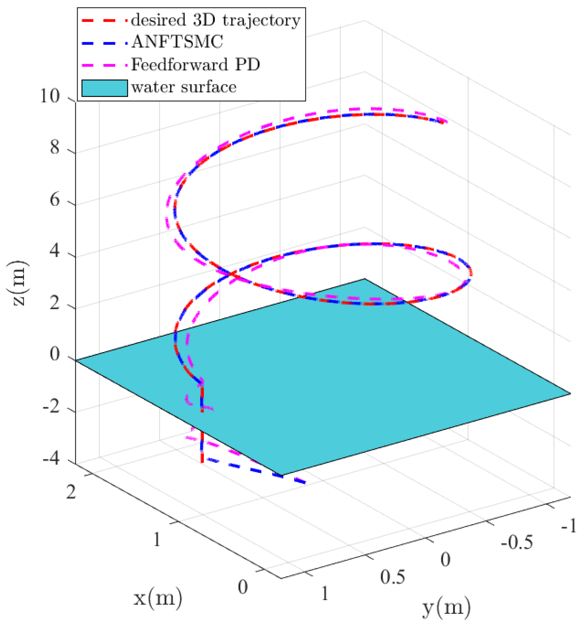
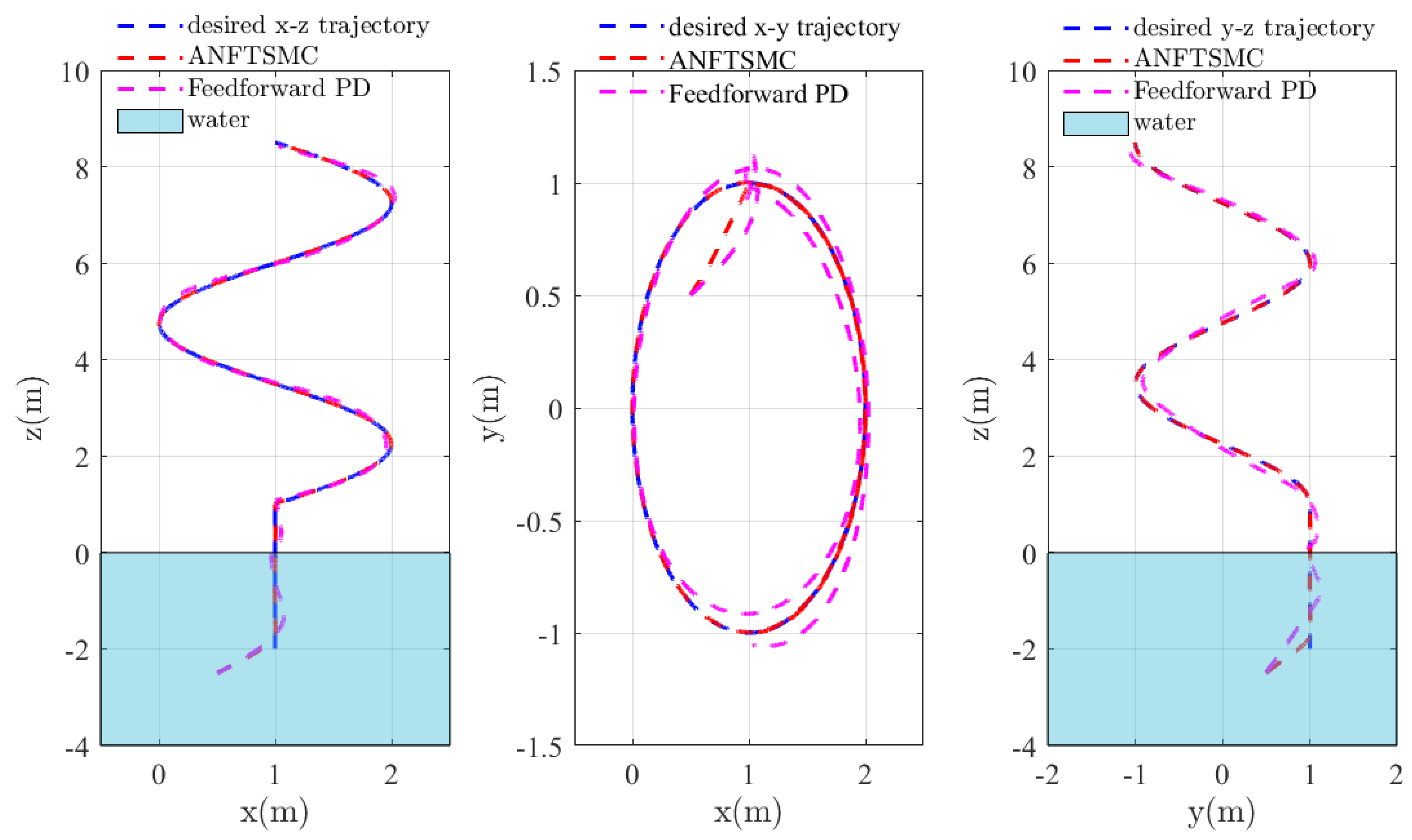
4.1. Simulation of the Vehicle Crossing the Water Surface for Takeoff

In the following simulation, the initial position and attitude of the HAUV are, respectively, selected to be $x_0=0.3$, $y_0=0.4$, $z_0=-2$, and ${\varphi }_0=0,{\theta }_0=0,{\psi }_0=0$.

To verify the robustness of the designed controller, the lumped uncertainty is reset as follows:

$$\begin{array}{l}{d}_x=0.3\times \left(cos\left(0.4t\right)+k_s\right),d_y=0.3\times \left(sin\left(0.5t\right)+k_s\right),d_z=0.3\times \left(sin\left(0.7t\right)+k_s\right)\hfill \\ d_{\varphi }=0.3\times \left(cos\left(0.4t\right)+k_s\right),d_{\theta }=0.3\times \left(sin\left(0.5t\right)+k_s\right),d_{\psi }=0.3\times \left(sin\left(0.7t\right)+k_s\right)\hfill \end{array}$$

(44)

The desired water-exit trajectory is determined using Equation (45):

$$x_d=\{\begin{array}{c}1,t\in \left[0,20\right)\\ sin\left(0.1\pi \left(t-20\right)\right),t\in \left[20,50\right]\end{array},y_d=\{\begin{array}{c}1,t\in \left[0,20\right)\\ cos\left(0.1\pi \left(t-20\right)\right),t\in \left[20,50\right]\end{array},z_d=\{\begin{array}{c}0.15t-2,t\in \left[0,20\right)\\ 0.25t-4,t\in \left[20,50\right]\end{array}$$

(45)

Autonomous takeoff and landing control remains a challenge for our designed coaxial HAUV because a water surface is usually not calm and complex sea conditions often stimulate compound disturbances to the vehicle. To reduce the difficulty faced by the HAUV when crossing disturbed water, we designed a piecewise trajectory. In the process of breaking through the trans-medium water surface, our trajectory is vertical, and the vertical climbing speed is selected to be small, at 0.15 m/s. After completely leaving the water surface, in order to prevent falls caused by the beating of wind and waves, we choose a higher climbing speed of 0.25 m/s to allow the HAUV to quickly escape from the near-water surface with a spiral trajectory.

In the position loop, the trajectory tracking performance of the HAUV based on the design control strategy is shown in Figure 4 and Figure 5. The simulation results show that the proposed method has strong robustness under complex interference. Meanwhile, the feedforward PD controller lacks robustness to disturbance, resulting in large fluctuations in trajectory tracking. The three subgraphs shown in Figure 4 describe the effect of position tracking in the $x$, $y$, and $z$ directions, respectively. As shown in Figure 4, we can see that the proposed position controller enables the HAUV to track the desired value quickly and accurately, even if the desired position changes rapidly. Figure 4 and Figure 5, respectively, show the effect of three-dimensional trajectory tracking and the effect of three sections. According to the effect of the coaxial HAUV tracking the desired trajectory, we can observe that the HAUV maneuvers from its initial point to the desired trajectory from under water, rises vertically through the water into the air, and, finally, performs an upward spiral maneuver in the air. The results show that the proposed controller can accurately track the specified trajectory instruction under conditions of parameter uncertainty and disturbance. Figure 6 shows the results of 2D planar trajectory tracking. It can be seen from the figure that there is a large deviation between the position of the vehicle and the expected position at the initial moment, but the position tracking approaches the expected trajectory within a very short time, which shows the good control accuracy of the ANFTSMC.

Figure 7 shows the attitude angle tracking effect of the HAUV. The yaw angle can be observed in the figure as being driven more quickly and accurately to the expected value because it does not have a degree of freedom coupled to the position loop. In addition, due to the large deviation between the initial position and the tracking position, the calculated expected roll angle and pitch angle produce large oscillations in the first few seconds and can be stabilized in a short time. In Figure 8, the simulation results show that the speed and accuracy of the feedforward PD controller are weaker than those of the ANFTSMC. As shown in Figure 8, the trajectory tracking errors and angle tracking errors converge to zero in a short time, and the tracking errors are stabilized in a small, bounded area near zero. Figure 9 shows the changes in the HAUV’s theoretical control input. It can be observed that the control signals are generally smooth (by means of an adaptive algorithm and by replacing the sign function in the controller with a saturation function). Furthermore, $u_1$ was small 13 s ago, which is due to buoyancy canceling out most of the gravity during underwater maneuvering. The HAUV has the characteristics of low energy consumption and strong maneuverability when under water. It has been proven that buoyancy generated by a HUAV’s watertight structure is of great significance and must be considered in controller design. $u_1$ mutates at around 13 s, at which time the HAUV is maneuvering through the water-air trans-medium process, and $u_1$ presents a linear increase trend and finally stabilizes, which is consistent with our linear hypothesis.

In addition, it can be clearly seen in Figure 10 and Figure 11 that the adaptive parameter estimation of the position ring and attitude ring is converging to a constant value, which guarantees the boundedness and convergence of the estimated parameters. Figure 12 shows the change curve of the non-singular fast terminal sliding-mode surface. As shown in Figure 12, the sliding-mode surface rapidly converges to zero, which means that the system error can quickly reach the sliding state, thereby verifying that the designed controller has the advantage of a fast response. In addition, Figure 13 shows the changing trend of the switching function after linearization. It can be observed that the switching process of the system model has been completed during the exiting-water process.

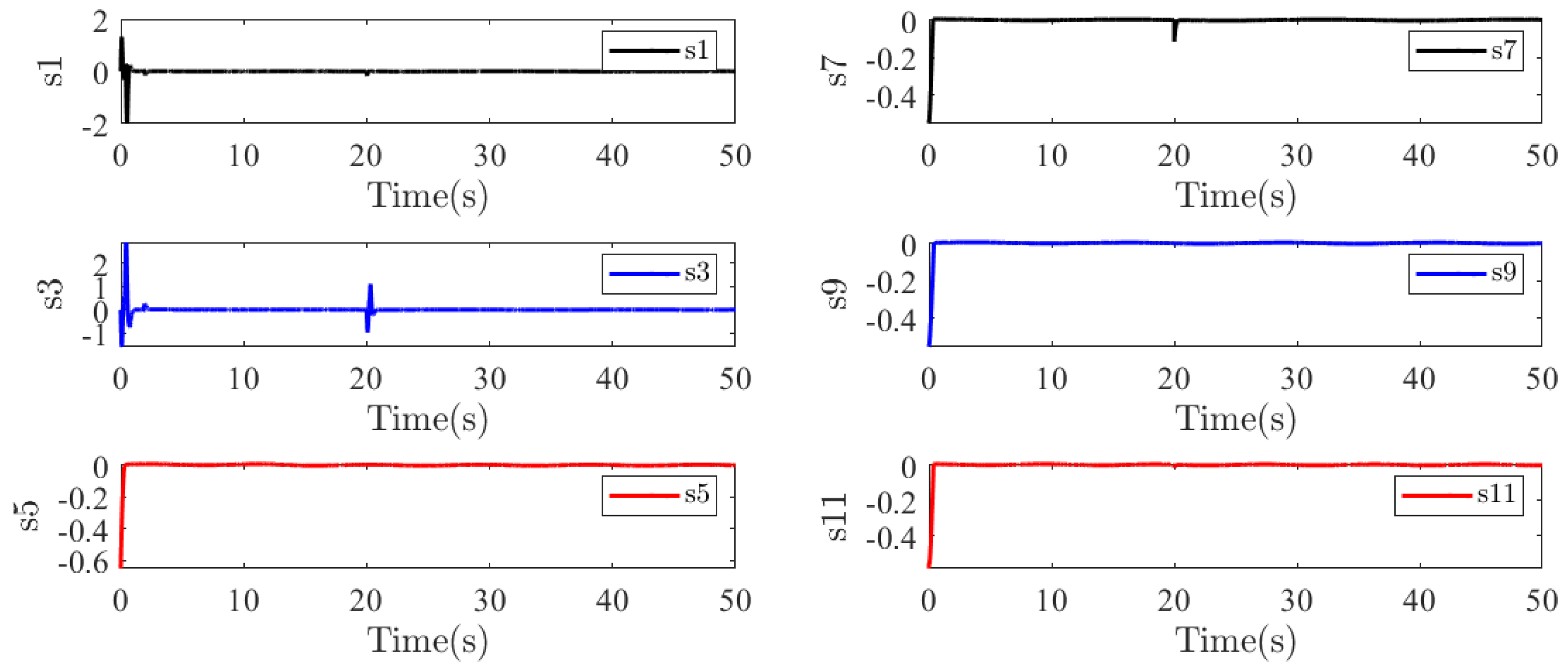
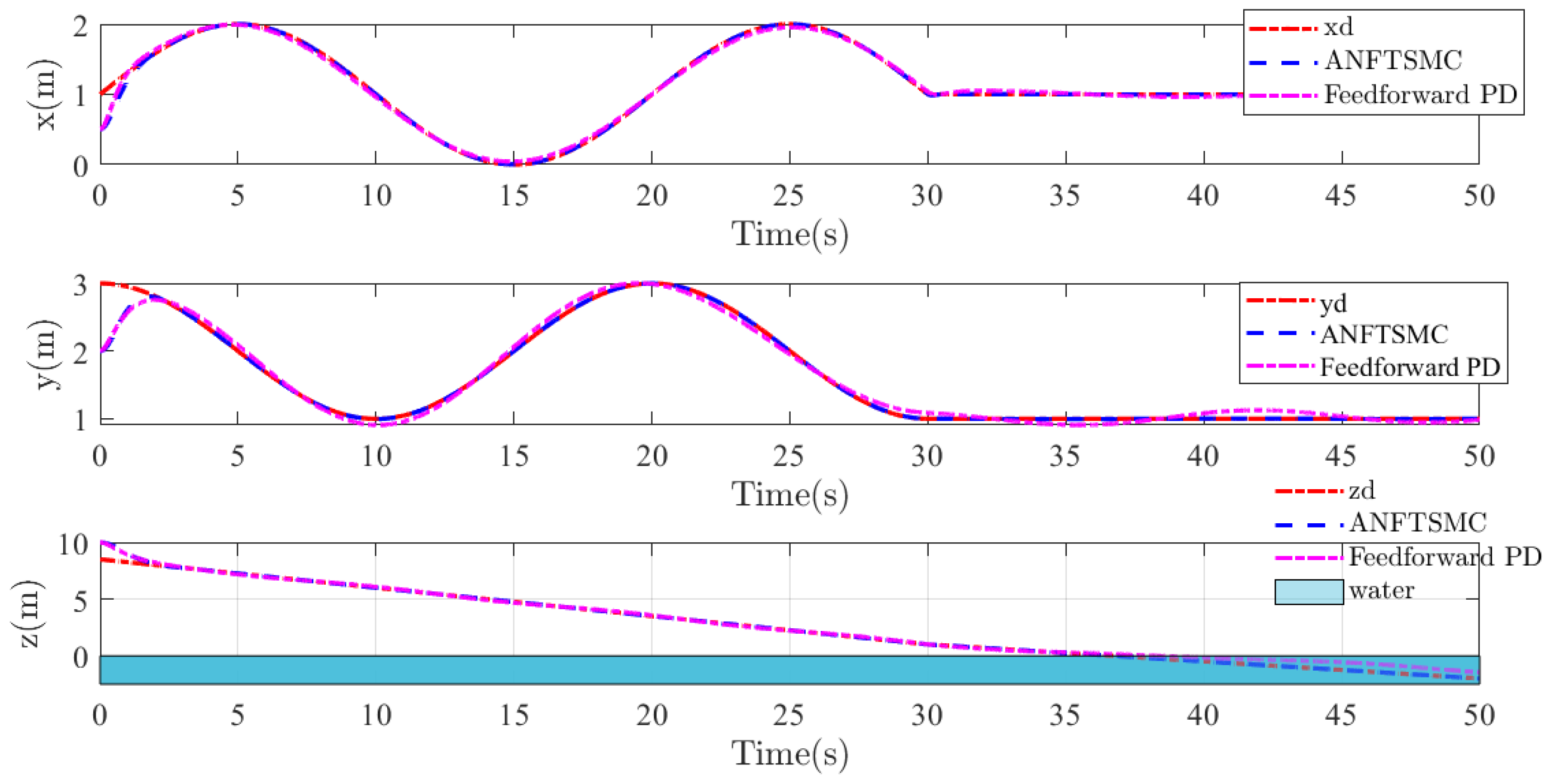
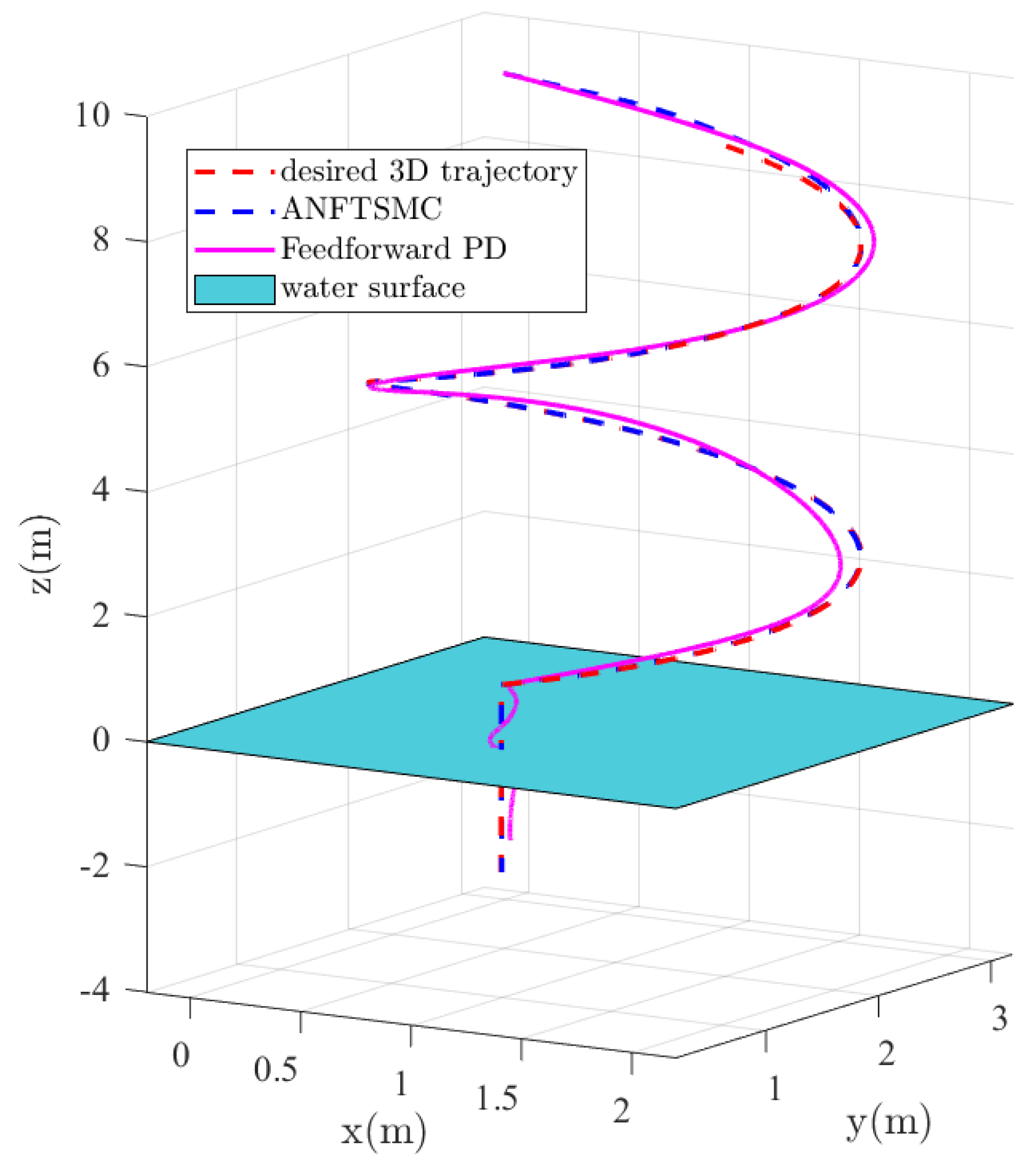
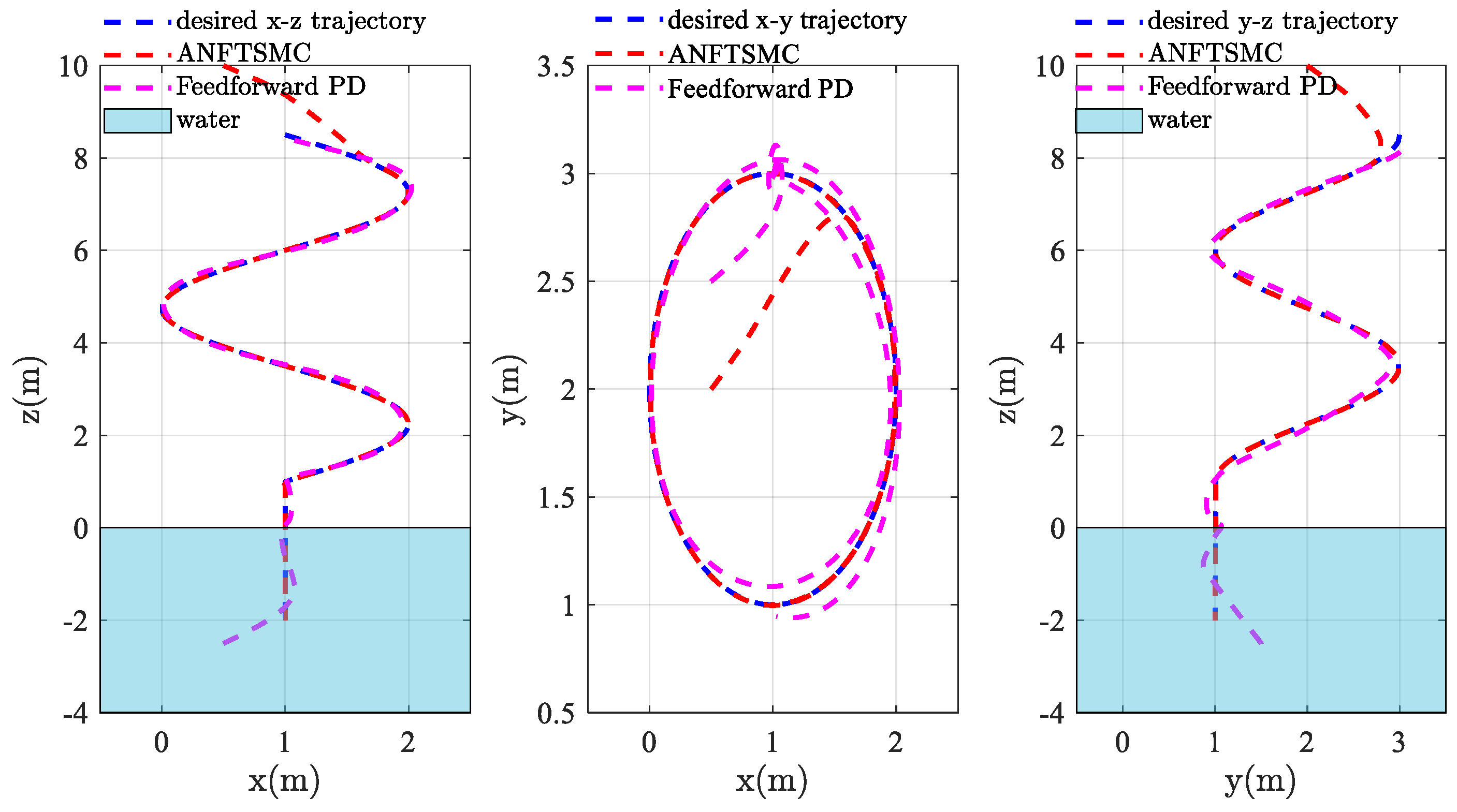
4.2. Simulation of the Vehicle Crossing the Water Surface during Diving

The simulation of the breakthrough trans-medium effluent has been discussed in detail in the previous section. In this section, we briefly describe the effectiveness of the controller we designed during the water-entry phase.

In the diving simulation, the initial position and the attitude of HAUV are set as $x_0=0.5$, $y_0=2$, $z_0=10$ and ${\varphi }_0=0,{\theta }_0=0,{\psi }_0=0$.

The water-entry path we designed is determined as follows:

$$x_d=\{\begin{array}{c}sin\left(0.1\pi t\right)+1,t\in \left[0,30\right)\\ 1,t\in \left[30,50\right]\end{array},y_d=\{\begin{array}{c}cos\left(0.1\pi t\right)+2,t\in \left[0,30\right)\\ 1,t\in \left[30,50\right]\end{array},z_d=\{\begin{array}{c}-0.25t+8.5,t\in \left[0,30\right)\\ -0.15t+5.5,t\in \left[30,50\right]\end{array}$$

(46)

According to the simulation results of trajectory tracking during the trans-medium process, as shown in Figure 14, Figure 15 and Figure 16, the vehicle first flies in a descending spiral arc in the air, gives up the horizontal maneuver at 1 m from the water surface, carries out a vertical landing and enters the water, and then dives vertically to 2 m below the water surface. The simulation process ends here. Based on the above results, by comparing the tracking effects of the two controllers, we can conclude that the ANFTSMC can more accurately return the aircraft from the air to the water.

In addition, Figure 17 shows that at 35–40 s, the attitude angle tracking error suddenly decreases after a sudden change, which is due to the trajectory switch at 30 s. Although the feedforward PD controller can also track the desired attitude angle, it is obvious that its reaction speed and control accuracy are weaker than those of the ANFTSMC designed by us. The control input of the vehicle is shown in Figure 18. In the initial phase, the upward thrust u1 is stable until t = 35 s. Then, as it begins to enter the water, the thrust decreases gradually, and at full immersion, the thrust stabilizes around a specific value and continues for some time. It is worth noting that the observations in Figure 19 and Figure 20 show that the estimates of the adaptive parameters still converge to a constant value, indicating that the upper bound of lumped uncertainty is effectively estimated.

5. Conclusions

In this paper, an additional variable, a linearized change function based on the high correlation between the vehicle body and water, is introduced, and a multi-modal HAUV motion model is integrated into a relatively accurate, continuous dynamic model. The model can be used in air flight, during underwater motion, and during trans-medium processes, and system instability caused by model mutation is avoided. To solve the HAUV’s trajectory tracking problem due to ocean disturbances and time-varying model parameters, a novel ANFTSMC technique is used to avoid the singularity problem of traditional TSMC. Based on the Lyapunov theory, the finite-time stability of the NFTSMC controller demonstrates the controllability and stability of the system, and the finite-time fast convergence of all state variables is realized. To reduce the adverse effect of buffeting on actuators in traditional SMC, an adaptive law is designed to estimate the upper bound of lumped uncertainty online in real time. The simulation results show that the proposed controller is feasible. The proposed method has good tracking ability, and the control errors converge to zero in a finite time.

In future work, the design and manufacture of the prototype will be further investigated, and the influence of real, random wind gusts and waves will be considered in combination with experimental methods to make the modeling more accurate. It is worth noting that the transient control performance at the water–air interface during the trans-medium process should also be seriously considered. The knock of high-speed rotating propellers on the water surface is very likely to cause takeoff failure. Therefore, a preset performance control algorithm will be developed in subsequent work. We will also attempt to use an interference observer or RBFNN technology to compensate for lumped uncertainty.

References

1. Liu, M.; Yang, S.; Li, H.; Xu, J.; Li, X. Energy Consumption Analysis and Optimization of the Deep-Sea Self-Sustaining Profile Buoy. Energies 2019, 12, 2316. [Google Scholar] [CrossRef] [Green Version]
2. Wu, H.; Niu, W.; Wang, S.; Yan, S. A feedback control strategy for improving the motion accuracy of underwater gliders in currents: Performance analysis and parameter optimization. Ocean. Eng. 2022, 252, 111250. [Google Scholar] [CrossRef]
3. Zhang, L.; Zheng, Y.; Huang, B.; Su, Y. Finite-time trajectory tracking control for under-actuated unmanned surface vessels with saturation constraint. Ocean. Eng. 2022, 249, 110745. [Google Scholar] [CrossRef]
4. Zhu, C.; Jun, L.; Huang, B.; Su, Y.; Zheng, Y. Trajectory tracking control for autonomous underwater vehicle based on rotation matrix attitude representation. Ocean. Eng. 2022, 252, 111206. [Google Scholar] [CrossRef]
5. Jacobs, T.; Jacobi, M.; Rogers, M.; Adams, J.; Coffey, J.J.; Walker, J.; Johnston, B. Testing and Evaluating Low Altitude Unmanned Aircraft System Technology for Maritime Domain Awareness and Oil Spill Response in the Arctic. Mar. Technol. Soc. J. 2015, 49, 145–150. [Google Scholar] [CrossRef] [Green Version]
6. Girdhar, Y.; Xu, A.; Shkurti, F.; Higuera, J.C.G.; Meghjani, M.; Giguere, P.; Rekleitis, I.; Dudek, G. Monitoring Marine Environments using a Team of Heterogeneous Robots. In Proceedings of the RSS 2012 Workshop on Robotics for Environmental Monitoring (WREM 2012), Vilamoura, Portugal, 7–12 October 2013. [Google Scholar]
7. Zeng, Z.; Lyu, C.; Bi, Y.; Jin, Y.; Lu, D.; Lian, L. Review of hybrid aerial underwater vehicle: Cross-domain mobility and transitions control. Ocean. Eng. 2022, 248, 110840. [Google Scholar] [CrossRef]
8. Petrov, G. Flying Submarine. J. Fleet 1995, 3, 52–53. Available online: http://www.airforce.ru/aircraft/miscellaneous/flying_submarine/index.htm (accessed on 24 June 2023).
9. Yao, G.; Li, Y.; Zhang, H.; Jiang, Y.; Wang, T.; Sun, F.; Yang, X. Review of hybrid aquatic-aerial vehicle (HAAV): Classifications, current status, applications, challenges and technology perspectives. Prog. Aerosp. Sci. 2023, 139, 100902. [Google Scholar] [CrossRef]
10. Drews, J.P.; Neto, A.A.; Campos, M. Hybrid Unmanned Aerial Underwater Vehicle: Modeling and Simulation. In Proceedings of the 2014 IEEE/RSJ International Conference on Intelligent Robots and Systems (IROS), Chicago, IL, USA, 14–18 September 2014. [Google Scholar]
11. Maia, M.M.; Mercado, D.A.; Diez, F.J. Design and implementation of multirotor aerial-underwater vehicles with experimental results. In Proceedings of the 2017 IEEE/RSJ International Conference on Intelligent Robots and Systems (IROS), Vancouver, BC, Canada, 24–28 September 2017. [Google Scholar]
12. Mercado, D.A.; Maia, M.M.; Diez, F.J. Aerial-underwater systems, a new paradigm in unmanned vehicles. In Proceedings of the 2017 International Conference on Unmanned Aircraft Systems (ICUAS), Miami, FL, USA, 13–16 June 2017. [Google Scholar]
13. Alzu’bi, H.; Mansour, I.; Rawashdeh, O. Loon copter: Implementation of a hybrid unmanned aquatic–aerial quadcopter with active buoyancy control. J. Field Robot. 2018, 35, 764–778. [Google Scholar] [CrossRef]
14. Qi, D.; Feng, J.; Li, Y. Dynamic model and ADRC of a novel water-air unmanned vehicle for water entry with in-ground effect. J. Vibroengineering 2016, 18, 3743–3756. [Google Scholar] [CrossRef] [Green Version]
15. Ma, Z.; Feng, J.; Jian, Y. Research on vertical air–water trans-media control of Hybrid Unmanned Aerial Underwater Vehicles based on adaptive sliding mode dynamical surface control. Int. J. Adv. Robot. Syst. 2018, 15, 172988141877053. [Google Scholar] [CrossRef] [Green Version]
16. Chen, Y.; Liu, Y.; Meng, Y.; Yu, S.; Zhuang, Y. System Modeling and Simulation of an Unmanned Aerial Underwater Vehicle. J. Mar. Sci. Eng. 2019, 7, 444. [Google Scholar] [CrossRef] [Green Version]
17. Zhang, H.; Zeng, Z.; Yu, C.; Jiang, Z.; Han, B.; Lian, L. Predictive and sliding mode cascade control for cross-domain locomotion of a coaxial aerial underwater vehicle with disturbances. Appl. Ocean. Res. 2020, 100, 102183. [Google Scholar] [CrossRef]
18. Chen, Q.; Zhu, D.; Liu, Z. Attitude control of aerial and underwater vehicles using single-input FUZZY P+ID controller. Applied Ocean. Res. 2020, 107, 102460. [Google Scholar] [CrossRef]
19. Lu, D.; Xiong, C.; Zeng, Z.; Lian, L. Adaptive Dynamic Surface Control for a Hybrid Aerial Underwater Vehicle With Parametric Dynamics and Uncertainties. IEEE J. Ocean. Eng. 2019, 45, 740–758. [Google Scholar] [CrossRef]
20. Lu, D.; Guo, Y.; Xiong, C.; Zeng, Z.; Lian, L. Takeoff and Landing Control of a Hybrid Aerial Underwater Vehicle on Disturbed Water’s Surface. IEEE J. Ocean. Eng. 2022, 47, 295–311. [Google Scholar] [CrossRef]
21. Bi, Y.; Lu, D.; Zeng, Z.; Lian, L. Dynamics and control of hybrid aerial underwater vehicle subject to disturbances. Ocean. Eng. 2022, 250, 110933. [Google Scholar] [CrossRef]
22. Tan, L.; Liang, S.; Su, H.; Qin, Z.; Li, L.; Huo, J. Research on Amphibious Multi-Rotor UAV Out-of-Water Control Based on ADRC. Appl. Sci. 2023, 13, 4900. [Google Scholar] [CrossRef]
23. Wei, T.; Hu, R.; Li, J.; Bi, Y.; Jin, Y.; Lu, D.; Zeng, Z.; Lian, L. Experimental study on trans-media hydrodynamics of a cylindrical hybrid unmanned aerial underwater vehicle. Ocean. Eng. 2022, 252, 111190. [Google Scholar] [CrossRef]
24. Wei, T.; Lu, D.; Zeng, Z.; Lian, L. Trans-Media Kinematic Stability Analysis for Hybrid Unmanned Aerial Underwater Vehicle. J. Mar. Sci. Eng. 2022, 10, 275. [Google Scholar] [CrossRef]
25. Wei, T.; Li, J.; Zeng, Z.; Lian, L. Trans-media resistance investigation of hybrid aerial underwater vehicle base on hydrodynamic experiments and machine learning. Ocean. Eng. 2022, 266, 112808. [Google Scholar] [CrossRef]
26. Gao, Y.; Zhang, H.; Yang, H.; Tan, S.; Gulliver, T.A.; Lu, T. Trans-Domain Amphibious Unmanned Platform Based on Coaxial Counter-Propellers: Design and Experimental Validation. IEEE Access 2021, 9, 149433–149446. [Google Scholar] [CrossRef]
27. Ravell, D.M.; Maia, M.M.; Diez, F.J. Modeling and control of unmanned aerial/underwater vehicles using hybrid control. Control Eng. Pract. 2018, 76, 112–122. [Google Scholar] [CrossRef]
28. Xu, J.; Hao, Y.; Wang, J.; Li, L. The Control Algorithm and Experimentation of Coaxial Rotor Aircraft Trajectory Tracking Based on Backstepping Sliding Mode. Aerospace 2021, 8, 337. [Google Scholar] [CrossRef]
29. Glida, H.E.; Chelihi, A.; Abdou, L.; Sentouh, C.; Perozzi, G. Trajectory tracking control of a coaxial rotor drone: Time-delay estimation-based optimal model-free fuzzy logic approach. ISA Trans. 2022, 137, 236–247. [Google Scholar] [CrossRef]
30. Mokhtari, M.R.; Braham, A.C.; Cherki, B. Extended state observer based control for coaxial-rotor UAV. ISA Trans. 2016, 61, 1–14. [Google Scholar] [CrossRef]
31. Labbadi, M.; Cherkaoui, M. Novel robust super twisting integral sliding mode controller for a quadrotor under external disturbances. Int. J. Dyn. Control 2020, 8, 805–815. [Google Scholar] [CrossRef]
32. Boukattaya, M.; Mezghani, N.; Damak, T. Adaptive nonsingular fast terminal sliding-mode control for the tracking problem of uncertain dynamical systems. Isa Trans. 2018, 77, 1–19. [Google Scholar] [CrossRef]
33. Labbadi, M.; Cherkaoui, M. Robust adaptive nonsingular fast terminal sliding-mode tracking control for an uncertain quadrotor UAV subjected to disturbances—ScienceDirect. ISA Trans. 2020, 99, 290–304. [Google Scholar] [CrossRef]
34. Huang, S.; Yang, Y. Adaptive neural-network-based nonsingular fast terminal sliding mode control for a quadrotor with dynamic uncertainty. Drones 2022, 6, 206. [Google Scholar] [CrossRef]
35. Asl, S.B.F.; Moosapour, S.S. Adaptive backstepping fast terminal sliding mode controller design for ducted fan engine of thrust-vectored aircraft. Aerosp. Sci. Technol. 2017, 71, 521–529. [Google Scholar]
36. Plestan, F.; Shtessel, Y.; Bregeault, V.; Poznyak, A. New methodologies for adaptive sliding mode control. Int. J. Control 2010, 83, 1907–1919. [Google Scholar] [CrossRef] [Green Version]
37. Moulay, E.; Perruquetti, W. Finite time stability and stabilization of a class of continuous systems. J. Math. Anal. Appl. 2006, 323, 1430–1443. [Google Scholar] [CrossRef] [Green Version]
38. Chen, L.; Liu, Z.; Gao, H.; Wang, G. Robust adaptive recursive sliding mode attitude control for a quadrotor with unknown disturbances. ISA Trans. 2022, 122, 114–125. [Google Scholar] [CrossRef]
Figure 1. Schematic diagram of two operation modes’ motion processes of the coaxial HAUV.
Applsci 13 08026 g001
Figure 2. The coaxial HAUV’s conceptual sketch and coordinate systems.
Applsci 13 08026 g002
Figure 3. Block diagram of the coaxial HAUV’s control structure.
Applsci 13 08026 g003
Figure 4. Effect of the coaxial HAUV’s position tracking.
Applsci 13 08026 g004
Figure 5. Effect of the coaxial HAUV’s 3D trajectory tracking when exiting water.
Applsci 13 08026 g005
Figure 6. Exiting-water tracking responses of the coaxial HAUV in the 2D plane.
Applsci 13 08026 g006
Figure 7. Attitude tracking effect during motion.
Applsci 13 08026 g007
Figure 8. Position and attitude tracking errors.
Applsci 13 08026 g008
Figure 9. Theoretical control input during the process of exiting water.
Applsci 13 08026 g009
Figure 10. Estimated values of the adaptive parameters of the attitude loop.
Applsci 13 08026 g010
Figure 11. Estimated values of the adaptive parameters of the position loop.
Applsci 13 08026 g011
Figure 12. Response of the NFTSMC surface during trans-medium motion.
Applsci 13 08026 g012
Figure 13. Variation of the linearized switch function.
Applsci 13 08026 g013
Figure 14. Tracking results of the HAUV’s actual position and expected position.
Applsci 13 08026 g014
Figure 15. Effect of the coaxial HAUV’s 3D water-entry trajectory tracking.
Applsci 13 08026 g015
Figure 16. Entry-water tracking responses of the coaxial HAUV in the 2D plane.
Applsci 13 08026 g016
Figure 17. Attitude response when tracking the desired trajectory.
Applsci 13 08026 g017
Figure 18. Theoretical control input of the water-entry process.
Applsci 13 08026 g018
Figure 19. Estimated values of the adaptive parameters of the position loop.
Applsci 13 08026 g019
Figure 20. Estimated values of the adaptive parameters of the attitude loop.
Applsci 13 08026 g020