Analysis of the Influence and Propagation Law of Urban Rail Transit Disruptions: A Case Study of Beijing Rail Transit

Abstract

In the context of the network operation of urban rail transit systems, disruptions caused by signal interruptions influence not only the operation of the service at a single station but also the level of service of the whole network. Moreover, it is even possible to induce the cascading failure of the urban rail transit network. Therefore, it is essential to maintain the real-time dynamic monitoring of abnormal stations in urban rail transit systems for security reasons. Based on the large amounts of automated fare collection (AFC) data, a real-time calculation method to estimate the influence intensity of the passenger flow is presented, the spatiotemporal distribution of the influence characteristics is analyzed, and the propagation law of disruptions in the urban rail transit network is explored. First, the fluctuation threshold of passenger flow in a normal situation for all stations was calculated. Accordingly, abnormal stations influenced by the disruption were identified. Then, an evaluation method for calculating the influence intensity of the passenger flow was proposed. Finally, a real-world case study based on the Beijing rail transit system was conducted. All abnormal stations were identified dynamically and displayed in real time, and the distribution and propagation law of abnormal stations were constructed by spatiotemporal diagrams. The influence intensity of passenger flow was analyzed in detail from the perspective of the whole network and representative stations. The results revealed that transfer stations were more vulnerable to the effects of disruption, and the duration for which these stations were affected was longer than that of ordinary stations. Moreover, short-distance travelers were less affected by the disruption than long-distance travelers. The method proposed in this paper can provide a theoretical basis for rail management departments to grasp the characteristics of passenger flow in real time, formulate disposal measures dynamically, and provide more accurate information services for passengers.

1. Introduction

Urban rail transit has become one of the most crucial travel modes in metropolises due to its low energy consumption, low pollution, high safety, and reliability [1,2,3,4]. Although urban rail transit brings great convenience to travelers, it also encounters many potential risks in daily operation [5,6], such as signal interruption, equipment failure, natural disasters, terrorist attacks, and other emergencies. The signaling system is a very vulnerable part of an urban rail transit system. The disruptions of urban rail transit systems caused by signal interruptions account for the largest proportion of all emergencies [7]. Once a disruption occurs in an urban rail transit system, it affects the transit quality, increases passengers’ travel times, and changes their travel behavior. Transit quality is considered to play an important role in the policy decision-making related to public transit [8,9,10,11]. With the increasing complexity of the urban rail transit network and the increase in correlation between different lines, the security and quality assessment of the urban rail transit network are of significant concern.

The urban rail transit network is a relatively closed system with a high population density, which makes it different from the urban road transportation system [12,13,14,15]. Once rail transit disruption occurs, the impact caused by the disruption propagates along the urban rail transit lines. However, most urban rail transit operators monitor emergencies through the manual observation of video surveillance [16] and accordingly determine flow restriction strategies at certain stations. This method is too subjective and also lacks theoretical support. In order to minimize the influence of emergencies on the urban rail transit system and resume operation as soon as possible, it is necessary to analyze the influence of passenger flow and the propagation law of disruptions. Based on the real-time analysis of the influence of passenger flow and the propagation law of disruptions, urban rail transit operators can quickly determine management measures.

The relevant literature on exploring the influence of emergencies on urban rail transit systems can be categorized into three directions. The first large stream of literature has paid attention to passenger behavior after emergencies. Dell’Olio et al. [17] explored the possible behavior of passengers and crew after an emergency in a rail transit system. Silva et al. [18] introduced the idea of statistics based on previous studies and developed a statistical method for analyzing the behavior of influenced passengers during the disruption of a section and the disruption of station operation. Furthermore, some studies have also focused on the problem of passenger route choice during emergencies. Tsuchiya et al. [19] constructed an impact model of operation disruption on the travel path of passengers based on a travel time estimation model for passengers between adjacent stations and a passenger travel path decision model and realized the quantitative assessment of the influence of disruption. Li et al. [16] established multiple logistic regression models to analyze passenger travel behavior during emergencies. Arslan Asim et al. [20] constructed a mixed multinomial logit model to investigate transit customers’ mode choice behavior during light rail transit short-term planned service disruption. The behavior of passengers may differ depending on the property and the extent of the disruption. Sun et al. [21] divided and analyzed three types of abnormal passenger flow affected by disruptions, such as passengers who left the system, passengers who took detours, and passengers who were delayed but continued their travel. In addition, due to the difficulty in obtaining real-world data on urban rail transit, some studies have used simulation methods to model and simulate passenger behavior during disruptions [22,23].

The second large stream of literature has paid attention to the influence of emergencies on passenger flow. Several simulation methods have been used to simulate different emergency scenarios and measure the influence of disruption on urban rail transit systems [23,24,25,26]. For example, Su et al. [23] analyzed the influence of disruption on passenger flow in an urban rail transit network by a simulation method. When the urban rail transit system was interrupted for a long time, a large number of passengers were stranded at stations. Gao et al. [27] used historical passenger flow data to estimate the stranded passenger flow at abnormal stations.

The third large stream of literature has paid attention to the evacuation of passengers after emergencies [28,29]. Zarboutis and Marmaras [28] studied the emergency evacuation of urban rail transit systems during fire scenarios. Jiang et al. [29] took the Beijing transit network as an example to simulate emergency evacuation at an urban metro station. Other scholars have aimed to investigate emergency response and bus bridging services [30,31,32,33]. Cadarso et al. [30] investigated how to recover from disruptions in an urban rail transit network. Cadarso and Marín [31] studied recovery from disruptions in rapid transit networks. In response to rail transit system disruptions, bus bridging services can evacuate stranded passengers and mitigate the adverse influence of disruptions. Liang et al. [32] developed a path-based multi-commodity flow formulation for bus bridging service design. However, the recovery time for disruptions may be uncertain. Tan et al. [33] provided an alternative scheme to evacuate passengers via the urban bus system considering an uncertain disruption recovery time and heterogeneous risk-taking behavior.

Previous studies have made great contributions to research on the impact of emergencies on urban rail transit. Most studies have paid attention to passenger behavior after emergencies and the evacuation of passengers. A few studies have focused on the influence of emergencies on passenger flow. Calculating the real-time influence intensity of passenger flow at each station and analyzing the propagation law of disruptions in urban rail transit networks are prerequisites for urban rail transit managers to determine rational strategies. Due to the difficulty in obtaining real-world data on urban rail transit and the complexity of passengers’ choice behavior, most studies have used simulation methods to analyze the influence of disruptions on passenger flow. However, since simulation methods are affected by parameter calibration and assumptions, the results of the propagation law of urban rail transit disruptions may be inconsistent with real-world situations. This approach is not suitable for real-time dynamic passenger flow monitoring when disruptions occur.

Based on previous studies, after assuming that the passenger flow at each station in a normal situation meets normal distribution, we proposed a method for calculating the influence intensity of passenger flow at abnormal stations during disruptions and analyzed the spatiotemporal distribution of the influence characteristics. Our contributions herein are summarized below.

First, based on the large amounts of AFC data for Beijing rail transit, we calculated and displayed the fluctuation threshold of the tap-in passenger flow during the normal operation of the urban rail transit system. Accordingly, a practical method to identify abnormal stations affected by disruptions was proposed.

Second, this paper presents a real-time calculation method for the intensity of passenger flow affected by disruptions at abnormal stations. The influence intensity of the tap-in passenger flow at abnormal stations was calculated and displayed in real time. Since the proposed method relies on only real-time AFC data, it is simple and easy to apply in the daily operation of any urban rail transit system. Moreover, it is suitable for the real-time monitoring and dynamic identification of daily operational risks. It can effectively improve the intelligent management of urban rail transit systems.

Third, we systematically analyzed the propagation law of disruptions in the urban rail transit network. At the macro level, spatiotemporal distribution diagrams were used to explore the propagation law of disruptions in the urban rail transit network. At the micro level, a more detailed analysis of the passenger flow at three types of representative stations was conducted.

The remainder of this study is organized as follows. In Section 2, methods for identifying abnormal stations and estimating influence intensity are provided. Section 3 presents a case study based on AFC data of Beijing rail transit to illustrate the validity of the proposed methods. Section 4 concludes this study.

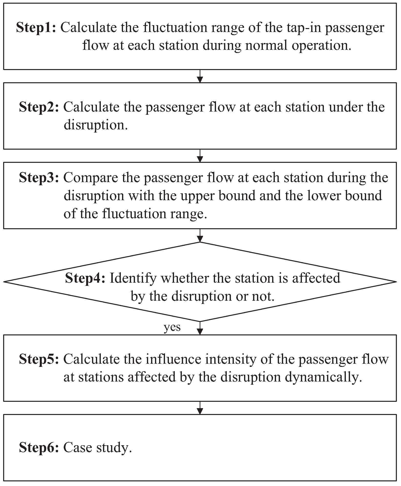
2. Identification of Abnormal Stations and Estimation of Influence Intensity

In this section, the method for identifying abnormal stations affected by urban rail transit disruptions is first presented in Section 2.1. Then, the estimation method for the influence intensity of urban rail transit disruptions is explored in Section 2.2.

2.1. Identification of Stations Affected by Disruptions

The tap-in passenger flow at stations is an important index to measure whether stations are operating normally. Generally, the tap-in passenger flow at stations fluctuates within a certain range. When the tap-in passenger flow at a station exceeds this range, a disruption may have occurred. Therefore, in order to identify the stations affected by a disruption, it is essential to obtain the fluctuation range of the tap-in passenger flow at stations during normal operation.

According to the statistical concept of normal distribution [21], if a variable meets normal distribution $x\sim (\mu ,\sigma )$, then the $3\sigma$ principle must be satisfied as follows:

$$\begin{array}{c}\hfill P\{\mu -3\sigma <x<\mu +3\sigma \}=99.74\%\end{array}$$

(1)

where $\mu$ is the mean value, and $\sigma$ is the variance.

After assuming that the tap-in passenger flow at each station in a normal situation meets normal distribution, the fluctuation range of the tap-in passenger flow during normal operation can be determined. Specifically, if the tap-in passenger flow at a station varies within the range $[\mu -3\sigma ,\mu +3\sigma ]$, this indicates that the station is in a normal situation; otherwise, it is in an abnormal situation.

2.2. Influence Intensity of Passenger Flow at Stations

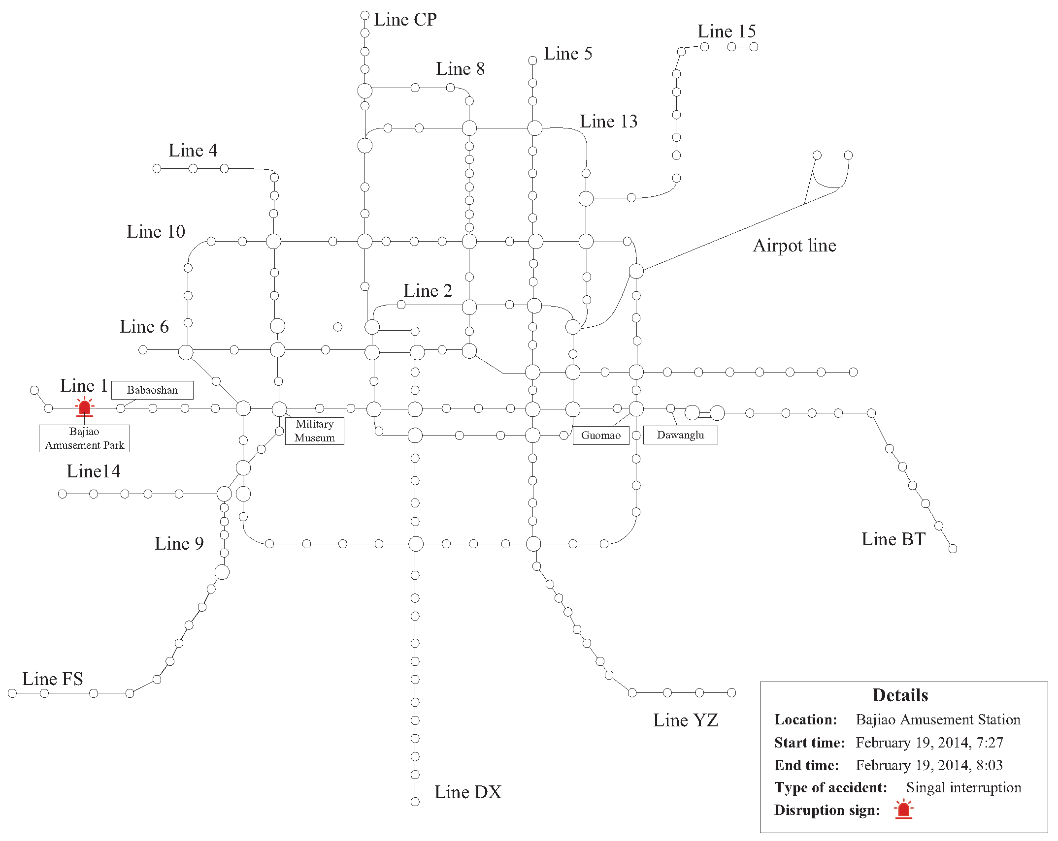
After determining the stations affected by the disruption, the law of propagation during the disruption needs to be further analyzed. Therefore, it is necessary to calculate the intensity of the impact on the tap-in passenger flow at abnormal stations due to the disruption (the influence intensity for short) during different time periods. Because the passenger flow data of each station are collected and uploaded every 15 min by the AFC system, many studies have used a period of 15 min to count or predict passenger flow in urban rail transit systems [6,21,34,35,36]. In this study, the tap-in passenger flow for a period of 15 min at each station was counted.

Let i denote a station and j denote a 15 min period. $R_{ij}$ represents the influence intensity of the tap-in passenger flow for time period j at station i affected by the disruption. $x_{ij}$ is the tap-in passenger flow for time period j at station i.

As described in Section 2.1, the passenger flow at each station fluctuates within a range during normal operation. The lower bound and upper bound of the tap-in passenger flow for a certain period at a certain station can be calculated by Equation (1), which can be represented by ${\lambda }_{ij}^{min}$ and ${\lambda }_{ij}^{max}$, respectively. When a station is affected by a disruption, the exact amount of passenger flow during normal operation cannot be determined. It may be equal to any value within the fluctuation range. Therefore, the influence intensity of the tap-in passenger flow should be within a certain range $[R_{ij}^{min},R_{ij}^{max}]$, which can be calculated by:

$$\begin{array}{c}\hfill R_{ij}^{max}=\frac{\left|x_{ij}-{\lambda }_{ij}^{max}\right|}{{\lambda }_{ij}^{max}},\forall i\in N,j\in J\end{array}$$

(2)

$$\begin{array}{c}\hfill R_{ij}^{min}=\frac{\left|x_{ij}-{\lambda }_{ij}^{min}\right|}{{\lambda }_{ij}^{min}},\forall i\in N,j\in J\end{array}$$

(3)

where N denotes the set of stations, and J denotes the set of time periods.

To enhance the readability and summarize the method, a flow chart of the proposed method is illustrated in Figure 1.

3. Case Study

3.1. Data Description

A real-world case study based on Beijing rail transit is presented below. There were 17 lines and 236 stations in the Beijing rail transit system in 2014. The AFC data of the Beijing rail transit system for 8 working days in 2014 were collected, namely, 19 February, 26 February, 5 March, 12 March, 19 March, 26 March, 2 April, and 9 April.

Line 1 is the main rail transit line in the Beijing rail transit system. It crosses the whole central urban area and undertakes important passenger transportation tasks in the morning and evening rush hour. Moreover, line 1 closely links residents living in the east and west areas of Beijing. On 19 February, a signal interruption occurred at Bajiao Amusement Park station on line 1 between 7:27 a.m. and 8:03 a.m. It affected the operation of adjacent stations and the regional networks, which caused 30 trains to be stopped and 5 trains to be turned back halfway. The Beijing rail transit network and the location of the disruption are illustrated in Figure 2. No signal interruption occurred on the other days.

Before identifying the abnormal stations of the rail transit system and calculating the influence intensity, data cleaning was conducted, that is, eliminating abnormal data and data irrelevant to this study, such as the data on the transaction type, card type, and ticket type. Then, the large amounts of real-time AFC data for the urban rail transit network were processed and counted by MATLAB, and the tap-in passenger flow distribution of each station was obtained at a 15 min granularity.

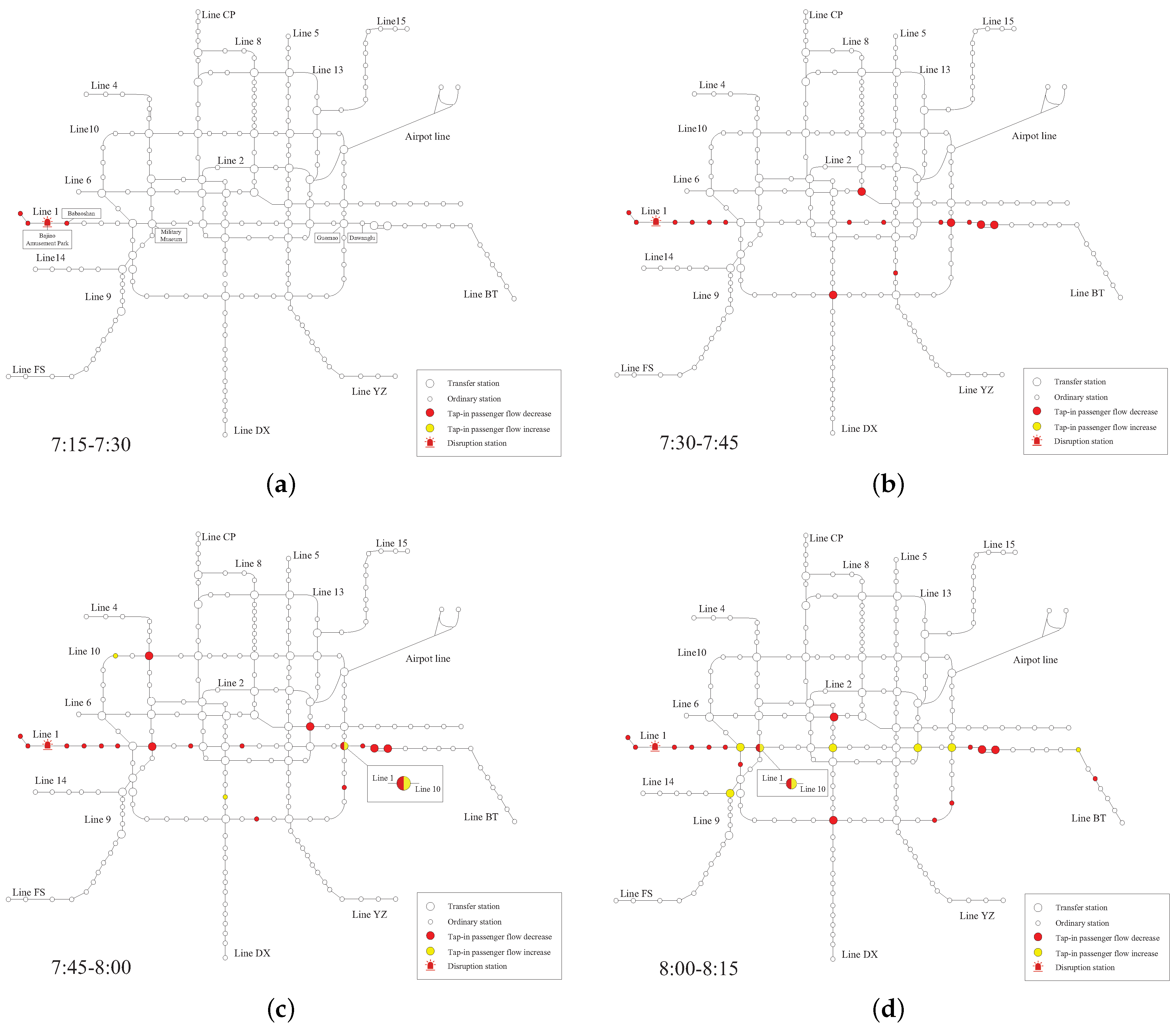
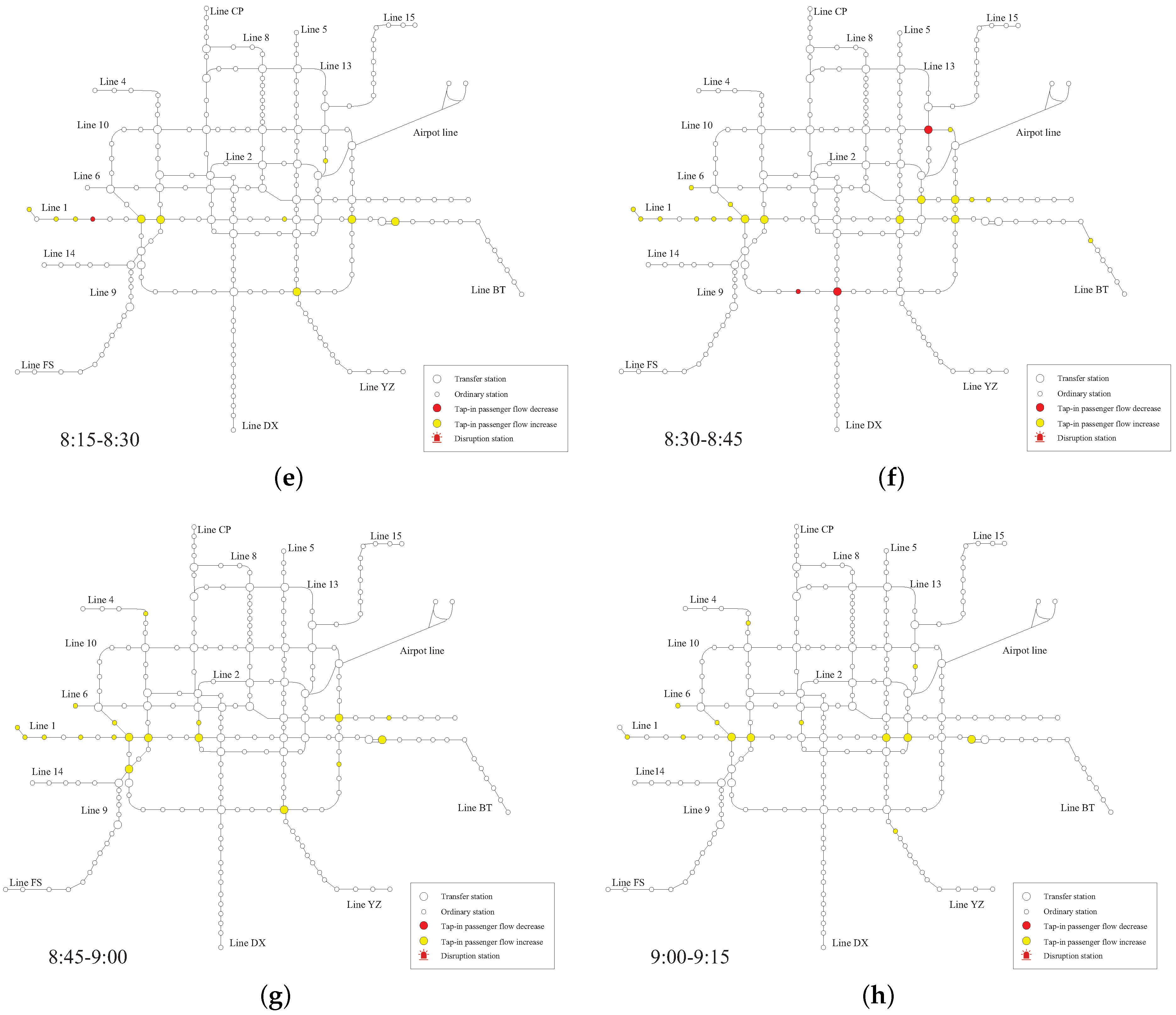
3.2. Results and Analysis of Abnormal Stations

In this subsection, the fluctuation threshold of the tap-in passenger flow during normal operation for all stations in the network is calculated according to the method proposed in Section 2.1. All abnormal stations affected by the disruption were identified and displayed with spatiotemporal diagrams. Some representative ordinary stations and transfer stations in the Beijing rail transit network were selected for a comparative analysis.

3.2.1. Analysis of Abnormal Stations in the Whole Network

According to the $3\sigma$ principle, the fluctuation threshold of the tap-in passenger flow at all stations during the normal operation was obtained. Then, after comparing the tap-in passenger flow between 7:00 a.m. and 10:00 a.m. on 19 February with that during normal operation, all abnormal stations were identified, as shown in

Table 1. Number of abnormal stations affected by the disruption.

Time Period	Number of Abnormal Stations	Number of Stations with Decreased Tap-In Passenger Flow	Number of Stations with Increased Tap-In Passenger Flow
7:00–7:15	3	3	0
7:15–7:30	19	18	1
7:30–7:45	25	24	1
7:45–8:00	23	20	3
8:00–8:15	29	20	9
8:15–8:30	15	3	12
8:30–8:45	24	6	18
8:45–9:00	22	3	19
9:00–9:15	13	0	13
9:15–9:30	8	4	4
9:30–9:45	10	6	4
9:45–10:00	9	4	5

. It was found that the number of abnormal stations in the whole network increased first and then decreased from 7:00 a.m. to 10:00 a.m. Among all time periods, the number of abnormal stations between 8:00 a.m. and 8:15 a.m. was the highest, with 29 abnormal stations, of which 20 stations presented a decrease in tap-in passenger flow and 9 stations presented an increase in tap-in passenger flow. Moreover, in the early stage of the disruption, the abnormal stations were mainly characterized by a decreased tap-in passenger flow, while in the later stage, the abnormal stations were mainly characterized by an increased tap-in passenger flow.

To visualize the abnormal stations affected by the disruption, a spatiotemporal diagram was drawn, indicating the location of these abnormal stations during different time periods, as presented in Figure 3. It can be seen from Figure 3a that when the disruption occurred, the first stations to be affected were only those upstream and downstream of Bajiao Amusement Park station. Then, several stations adjacent to Bajiao Amusement Park station were affected by the disruption. Finally, the influence of the disruption gradually propagated from adjacent stations to some stations on line 1 that were far away from the disrupted station as time passed. The tap-in passenger flow at these stations decreased significantly. Generally, the disruption did not affect ordinary stations on other lines. It can be seen from Figure 3c that, at 7:45–8:00 a.m., some ordinary stations on line 1 that were far from the disrupted station were not affected by the disruption any longer. At 45 min after the disruption, the issue of signal interruption had been well resolved. The tap-in passenger flow at most transfer stations that were affected by the disruption began to increase, as shown in Figure 3d. Meanwhile, the passenger flow at ordinary stations that were far from the disruption station recovered to a normal level. In contrast to the transfer stations, these ordinary stations did not suffer an increased tap-in passenger flow. However, the adjacent stations were still suffering a decreased tap-in passenger flow in the meanwhile. As time passed, all stations returned to normal, except for the transfer stations affected by the disruption, as can be seen in Figure 3e–h. This indicates that the duration for which transfer stations were affected by the disruption was the longest. In summary, all stations affected by the disruption were ranked according to their recovery speed, from fastest to slowest, as follows: ordinary stations that were far away from the disrupted station, adjacent stations, and transfer stations. Since there was a significant difference between ordinary stations and transfer stations in terms of recovery speed, a detailed analysis of the two types of stations will be presented in the following subsection.

3.2.2. Analysis of Representative Ordinary Stations

Babaoshan station (close to the disrupted station) and Dawanglu station (far away from the disrupted station) are two ordinary stations on line 1 that were selected as representatives to analyze the calculation results of the fluctuation range of the tap-in passenger flow. The fluctuation curve of the tap-in passenger flow from 7:00 a.m. to 10:00 a.m. at Babaoshan station and Dawanglu station are shown in Figure 4a and Figure 4b, respectively.

It was found that the period for which Babaoshan station was affected by the disruption was from 7:15 a.m. to 8:30 a.m. Then, the passenger flow increased rapidly at 8:30 a.m., and the amount of tap-in passenger flow was even greater than the normal range. This was because some passengers chose to wait outside the station during the disruption and to continue their travel once the disruption was resolved. Finally, the tap-in passenger flow returned to normal after 8:35 a.m. The trend of the fluctuation in tap-in passenger flow at Dawanglu station was the same as that at Babaoshan station. However, due to the long distance between Dawanglu station and Bajiao Amusement Park station, where the disruption occurred, the period for which Dawanglu station was affected by the disruption was from 7:30 a.m. to 8:30 am. This showed a significant lag compared to Babaoshan station.

3.2.3. Analysis of Representative Transfer Stations

Here, several representative transfer stations were selected to analyze the fluctuation in tap-in passenger flow when the disruption occurred. Military Museum station is a transfer station on line 1 and line 9 that was close to the disrupted station. Another transfer station is Guomao station on line 1 and line 10, which was far away from the disruption station. The fluctuation curve of tap-in passenger flow from 7:00 a.m. to 10:00 a.m. at Military Museum station and Guomao station are shown in Figure 5.

As shown in Figure 5, the period for which transfer stations were affected by the disruption was from 7:45 a.m. to 9:15 a.m., which was significantly longer than that for ordinary stations (Section 3.2.2). The trends of the fluctuation curve of tap-in passenger flow at Military Museum station and Guomao Station were the same. Specifically, the tap-in passenger flow at transfer stations on line 1 decreased significantly after the disruption occurred, while the tap-in passenger flow at transfer stations on line 9 and line 10 increased significantly after the disruption occurred. This indicated that many travelers changed their travel routes from origins to destinations.

3.3. Analysis of Influence Intensity

Based on the identification of abnormal stations affected by the disruption, the influence intensity of abnormal stations was further analyzed from the perspectives of the whole network and several representative stations.

3.3.1. Influence Intensity Analysis from the Perspective of the Whole Network

As mentioned in Section 3.2, the number of stations that were affected by the disruption was the highest at 8:00–8:15 a.m. In order to compare the influence intensity of passenger flow at different stations, the upper bound of the tap-in passenger flow in Equation (2) was replaced with the mean value of the tap-in passenger flow for a certain period at a certain station. Then, the influence intensity of passenger flow at all stations at 8:00–8:15 a.m. was calculated, and the results of the top 15 stations according to the value of influence intensity are shown in

Table 2. Ranking of influence intensity of passenger flow at stations for 8:00-8:15 am.

Ranking	Station	Influence Intensity
1	Guchenglu	0.85
2	Yuquanlu	0.81
3	Sihui	0.77
4	Dawanglu	0.69
5	Military Museum (line 1)	0.67
6	Guomao (line 1)	0.55
7	Pingguoyuan	0.55
8	Wukesong	0.51
9	Sihui East	0.44
10	Gongzhufen	0.41
11	Ti’anmen West	0.40
12	Tongzhoubeiyuan	0.39
13	Babaoshan	0.35
14	Military Museum (line 9)	0.29
15	Nanfaxin	0.29

.

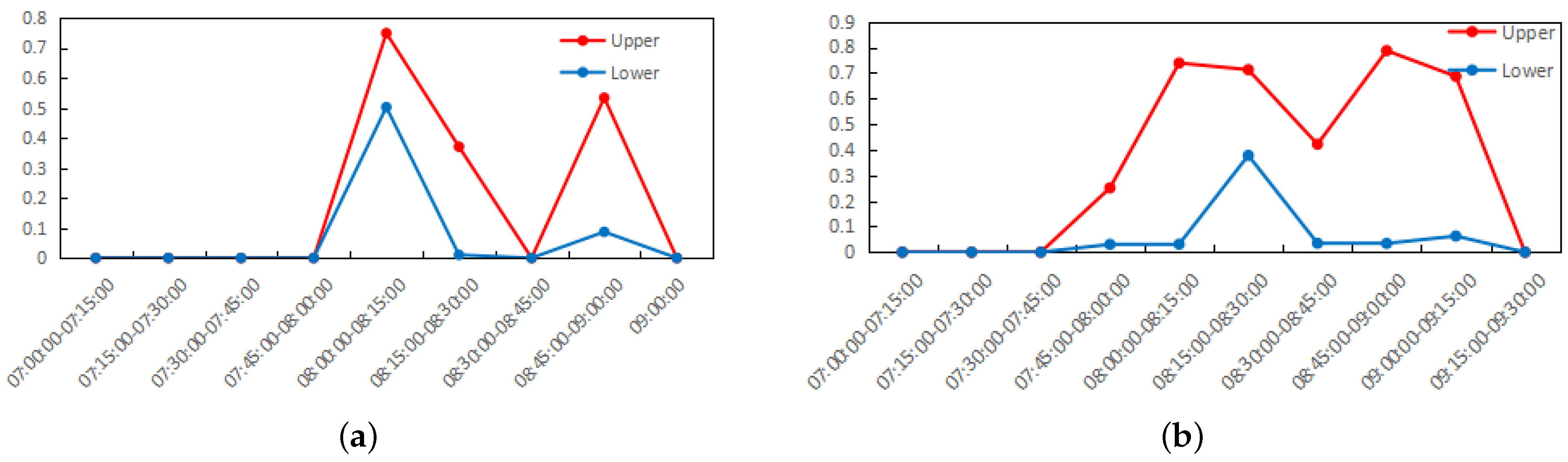
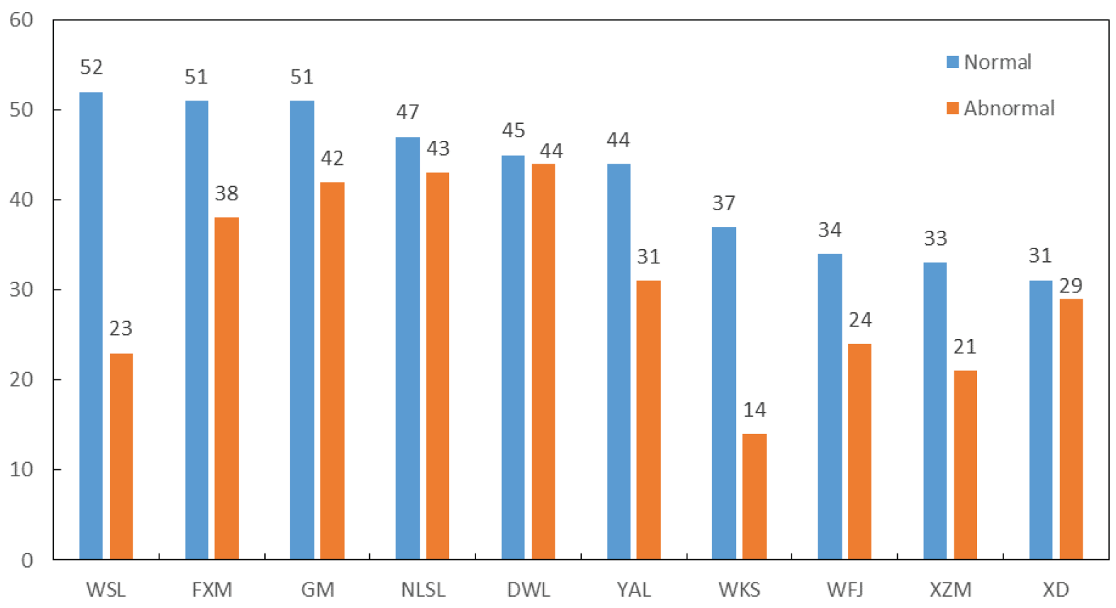
3.3.2. Influence Intensity Analysis from the Perspective of Representative Stations

Babaoshan station and Military Museum station were selected as a representative ordinary station and transfer station, respectively, for comparative analysis. The variation in the influence intensity at these two stations is illustrated in Figure 6 and Figure 7, respectively.

As shown in Figure 6, the influence intensity at Babaoshan station increased from 7:30 a.m. to 8:00 a.m. After the disruption was resolved, the influence intensity gradually decreased until 8:45 a.m. The variation in the influence intensity at Military Museum station was more severe and complex, presenting an “M” shape, as shown in Figure 7. The maximum influence intensity at Military Museum station on line 1 and line 9 occurred at around 8:00–8:15 a.m. and 8:45–9:00 a.m., respectively. The influence intensity gradually decreased after 9:00 a.m.

3.4. Analysis of Influenced OD Passenger Flow

When an urban rail transit system is disrupted, many passengers are forced to change their travel routes, as described in Section 3.2. Moreover, there are many travelers who may have to change their original station and destination station. This means that the origin–destination (OD) passenger flow may be affected by the disruption. Based on the identification of abnormal stations and the estimation of influence intensity in Section 3.2 and Section 3.3, the OD passenger flow at three stations representative of different station types were analyzed in detail: (1) disrupted station: Bajiao Amusement Park station; (2) ordinary station affected by the disruption: Babaoshan station; (3) transfer station affected by the disruption: Military Museum station.

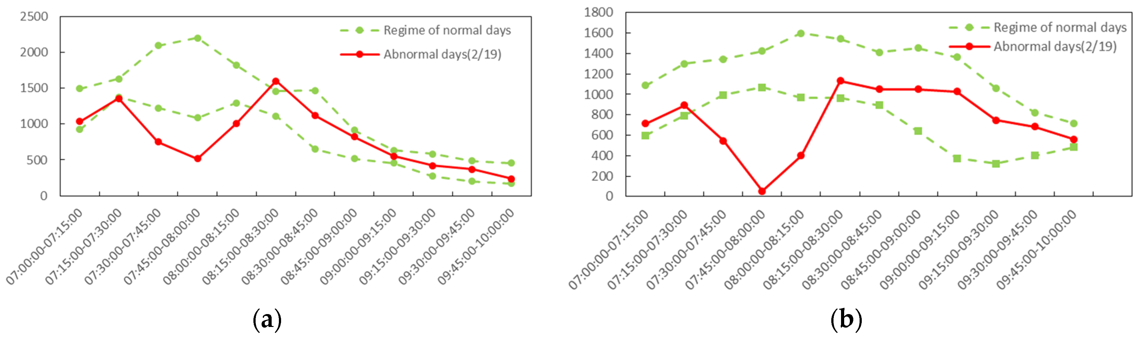
3.4.1. OD Passenger Flow at the Station with the Disruption

Bajiao Amusement Park station, which was the disrupted station, is an important station for residents in western Beijing. To analyze the influence of the disruption on the OD passenger flow at Bajiao Amusement Park station, taking this station as the origin, destination stations were ranked according to the OD passenger flow, and the top ten destination stations were selected. The OD passenger flow corresponding to the top ten destination stations is illustrated in Figure 8. It was found that the travel destinations of passengers at Bajiao Amusement Park station were mainly the business district and office area. Among the top ten destination stations, the distance from Bajiao Amusement Park station to Wanshoulu (WSL) station and Wukesong (WKS) station is short, and the travel time is within 15 min, while the distance from Bajiao Amusement Park station to other stations is relatively long.

As shown in Figure 8, all OD passenger flow at Bajiao Amusement Park station decreased due to the disruption. Compared with the long-distance travel demand, the short-distance travel demand was more affected by the disruption because it was more convenient for passengers to choose ground-level transportation as an alternative to continue their travel after the disruption. However, long-distance ground-level transportation is not as efficient as urban rail transit in terms of travel time, which led to more long-distance passengers choosing to wait outside the station and continue their travel after the disruption was resolved.

3.4.2. OD Passenger Flow at an Ordinary Station

Babaoshan station, which was the station downstream of the disrupted station, and its abnormality were analyzed in Section 3.2.2. The tap-in passenger flow at Babaoshan station at 7:00–9:00 a.m. is listed in

Table 3. The tap-in passenger flow at Babaoshan station.

Time Period	Upper Bound	Lower Bound	Tap-In Passenger Flow	Decreased Passenger Flow	Increased Passenger Flow
7:00–7:15	1495	925	1034	0	0
7:15–7:30	1632	1379	1355	24	0
7:30–7:45	2097	1223	752	471	0
7:45–8:00	2202	1088	515	573	0
8:00–8:15	1821	1295	1009	286	0
8:15–8:30	1457	1112	1604	0	147
8:30–8:45	1468	647	1116	0	0
8:45–9:00	917	520	825	0	0
Total				1354	147

. It can be seen that 1354 passengers were affected by the disruption, while only 147 passengers chose to wait outside the station.

To analyze the influence of the disruption on the OD passenger flow at Babaoshan station, taking this station as the origin, destination stations were ranked according to the OD passenger flow, and the top ten stations were selected. The OD passenger flow corresponding to the top ten destination stations is illustrated in Figure 9. Passengers who left the rail transit system and chose other travel modes mainly traveled short distances, such as to the FXM station or NLSL station. However, passengers traveling long distances chose to wait outside the station because ground-level transportation could not meet their travel purposes. Therefore, it was concluded that the occurrence of the disruption had a great influence on passenger delay for long-distance travel at the ordinary station.

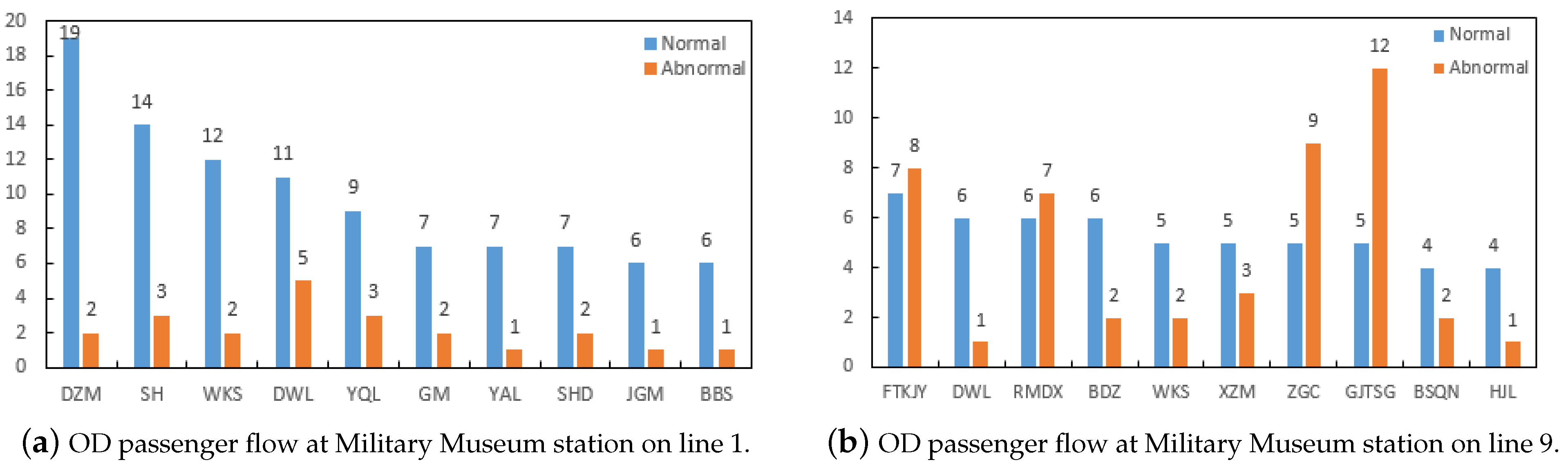
3.4.3. OD Passenger Flow at the Transfer Station

Military Museum station, which is the transfer station on line 1 and line 9, and its abnormality were analyzed in Section 3.2.3. The tap-in passenger flow of line 1 and line 9 at Military Museum station at 7:00-9:00 is shown in

Table 4. The tap-in passenger flow at Military Museum station on line 1.

Time Period	Upper Bound	Lower Bound	Tap-In Passengers	Decrease in Passengers	Increase in Passengers
7:00–7:15	224	141	151	0	0
7:15–7:30	237	179	190	0	0
7:30–7:45	298	236	253	0	0
7:45–8:00	326	242	253	0	0
8:00–8:15	346	175	87	88	0
8:15–8:30	266	196	269	0	3
8:30–8:45	256	161	241	0	0
8:45–9:00	183	130	199	0	0
Total				88	3

and

Table 5. The tap-in passenger flow at Military Museum station on line 9.

Time Period	Upper Bound	Lower Bound	Tap-In Passengers	Decrease in Passengers	Increase in Passengers
7:00–7:15	91	37	60	0	0
7:15–7:30	112	65	102	0	0
7:30–7:45	127	88	98	0	0
7:45–8:00	156	121	117	0	0
8:00–8:15	195	116	201	0	6
8:15–8:30	145	117	200	0	55
8:30–8:45	125	91	129	0	4
8:45–9:00	121	70	125	0	4
Total				0	69

, respectively. It can be seen that the passenger flow of line 1 at Military Museum station decreased by 88, while the passenger flow of line 9 at Military Museum station increased by 69. In other words, 78.41% of passengers chose to transfer to line 9 to continue their travel after the disruption, and 21.59% of the passengers chose to leave the rail transit system and continue to travel by other travel modes.

Similarly, the OD passenger flow at Military Museum station is shown in Figure 10. As a transfer station close to the disrupted station, the passenger flow at Military Museum station on line 1 significantly decreased after the disruption, and most of the passengers who exited the flow were short-distance travelers. On the contrary, the passenger flow at Military Museum station on line 9 increased because passengers chose to transfer to line 9 after the disruption. In general, the disruption had a great influence on the passengers traveling long distances at the transfer station. Due to the functions of the transfer station, the impact of the disruption propagated to the transfer line, which significantly increased the passenger flow on the transfer line.

4. Concluding Remarks

This paper proposed a method to identify abnormal stations and evaluate the intensity of passenger flow at abnormal stations affected by disruption. Then, the propagation law of the disruption in the urban rail transit network was analyzed based on large amounts of AFC data. Taking the Beijing rail transit system as a case study, all abnormal stations were dynamically identified, and the influence intensity of passenger flow at abnormal stations was also dynamically calculated. To enhance the readability, the spatiotemporal distribution characteristics of abnormal stations were analyzed at the macro level. At the micro level, the OD passenger flow at different types of representative stations with greater influence intensity after the disruption was analyzed in detail. A summary of the analysis of the influence and propagation law of urban rail transit disruptions is presented as follows:

(a) The proposed method relies on only real-time AFC data, making it simple and easy to implement in the daily operation of any urban rail transit system. It is suitable for the real-time monitoring and dynamic identification of the daily operational risks caused by disruptions in the context of network operation. Accordingly, it can effectively improve the intelligent management of urban rail transit systems.

(b) By analyzing the spatiotemporal distribution of abnormal stations in the network after the disruption, it was found that the first stations to be affected were those adjacent to the disrupted station. The tap-in passenger flow at these stations decreased significantly at the beginning of the disruption. Generally, the disruption did not affect ordinary stations on other lines. Moreover, all stations affected by the disruption could be sorted by their recovery speed, from fastest to slowest, as follows: ordinary stations that were far away from the disrupted station, adjacent stations, and transfer stations. The duration for which transfer stations were affected by the disruption was the longest. Furthermore, in contrast to transfer stations, ordinary stations affected by the disruption did not suffer an increased tap-in passenger flow after the disruption.

(c) At the disrupted station, some passengers chose to wait outside the station during the disruption and to continue their travel once the disruption was resolved. However, at ordinary stations far away from the disrupted station, passengers left the urban rail transit system (i.e., chose other travel modes, abandoned travel, etc.) rather than waiting outside the station during the disruption. Furthermore, at the transfer stations affected by the disruption, many travelers chose to change their travel routes from origins to destinations.

(d) Compared with the long-distance travel demand, the short-distance travel demand was more affected by the disruption because it was more convenient for passengers to choose ground-level transportation as an alternative to continue their travel after the disruption. However, long-distance ground-level transportation is not as efficient as urban rail transit in terms of travel time, which led to more long-distance passengers choosing to wait outside the station and continue their travel after the disruption was resolved.

However, this study had some limitations. The first limitation of our study was that the AFC data for the urban rail transit system were old. This was because the AFC data for urban rail transit are managed by government departments and operational agencies and are not open to the public. The report information on urban rail transit disruptions, such as when the disruption occurred, where it occurred, and how long it lasted, is also contained in confidential operational documents. The second limitation of our study was that we only analyzed a disruption caused by a signal interruption. We were unable to analyze other types of emergencies, such as equipment failure, natural disasters, and terrorist attacks. In the future, if we can obtain more recent data on different emergencies in urban rail transit systems, we will conduct more experiments to validate the method proposed in this study.

Further research work can be devoted to these extensions. First, the influence and propagation law of urban rail transit disruptions may vary from one city to another; therefore, more AFC data for different cities should be adopted in future studies. Second, the influence and propagation law of urban rail transit disruptions may also vary according to the type of emergency; therefore, AFC data on more types of emergencies in urban rail transit systems should be adopted in future studies. Third, more recent AFC data will be analyzed in future studies.

References

1. Ding, R.; Yin, J.; Dai, P.; Jiao, L.; Li, R.; Li, T.; Wu, J. Optimal topology of multilayer urban traffic networks. Complexity 2019, 2019, 1–19. [Google Scholar] [CrossRef]
2. Ding, R.; Zhang, T.; Zhou, T.; Zhang, Y.; Li, T.; Wu, J. Topologic characteristics and sustainable growth of worldwide urban rail networks. Int. J. Mod. Phys. B 2021, 35, 2150151. [Google Scholar] [CrossRef]
3. Dou, X.; Li, T. Multi-Objective Bus Timetable Coordination Considering Travel Time Uncertainty. Processes 2023, 11, 574. [Google Scholar] [CrossRef]
4. Li, T.; Chen, Y.; Wang, Z.; Liu, Z.; Ding, R.; Xue, S. Analysis of jobs-housing relationship and commuting characteristics around urban rail transit stations. IEEE Access 2019, 7, 175083–175092. [Google Scholar] [CrossRef]
5. Chen, Y.; Li, T.; Sun, Y.; Wu, J.; Guo, X.; Liu, D. Dynamic data-driven computation method for the number of waiting passengers and waiting time in the urban rail transit network. IET Intell. Transp. Syst. 2023, 17, 165–179. [Google Scholar] [CrossRef]
6. Yin, H.; Wu, J.; Liu, Z.; Yang, X.; Qu, Y.; Sun, H. Optimizing the release of passenger flow guidance information in urban rail transit network via agent-based simulation. Appl. Math. Model. 2019, 72, 337–355. [Google Scholar] [CrossRef]
7. Yin, J.; Ren, X.; Liu, R.; Tang, T.; Su, S. Quantitative analysis for resilience-based urban rail systems: A hybrid knowledge-based and data-driven approach. Reliab. Eng. Syst. Saf. 2022, 219, 108183. [Google Scholar] [CrossRef]
8. Nocera, S. An operational approach for quality evaluation in public transport services. Ing. Ferrov. 2010, 65, 363–383. [Google Scholar]
9. Nocera, S. The key role of quality assessment in public transport policy. Traffic Eng. Control 2011, 52, 394–398. [Google Scholar]
10. Xiong, J.; Huang, T.; Xu, Y.; Li, T.; Peng, F. Optimal network design of battery-powered electric feeder bus with determination of fleet size and number of chargers. J. Transp. Eng. Part A Syst. 2022, 148, 04021097. [Google Scholar] [CrossRef]
11. Li, T.; Xu, M.; Sun, H.; Xiong, J.; Dou, X. Stochastic ridesharing equilibrium problem with compensation optimization. Transp. Res. Part E Logist. Transp. Rev. 2023, 170, 102999. [Google Scholar] [CrossRef]
12. Li, T.; Wu, J.; Sun, H.; Gao, Z. Integrated co-evolution model of land use and traffic network design. Netw. Spat. Econ. 2016, 16, 579–603. [Google Scholar] [CrossRef]
13. Li, T.; Sun, H.; Wu, J.; Ge, Y.E. Optimal toll of new highway in the equilibrium framework of heterogeneous households’ residential location choice. Transp. Res. Part Policy Pract. 2017, 105, 123–137. [Google Scholar] [CrossRef]
14. Li, T.; Sun, H.; Wu, J.; Gao, Z.; Ge, Y.E.; Ding, R. Optimal urban expressway system in a transportation and land use interaction equilibrium framework. Transp. A Transp. Sci. 2019, 15, 1247–1277. [Google Scholar] [CrossRef]
15. Li, T.; Cao, Y.; Xu, M.; Sun, H. Optimal intersection design and signal setting in a transportation network with mixed HVs and CAVs. Transp. Res. Part E Logist. Transp. Rev. 2023, 175, 103173. [Google Scholar] [CrossRef]
16. Li, W.; Zhou, M.; Dong, H. Cpt model-based prediction of the temporal and spatial distributions of passenger flow for urban rail transit under emergency conditions. J. Adv. Transp. 2020, 2020, 8850541. [Google Scholar] [CrossRef]
17. Dell’Olio, L.; Ibeas, A.; Barreda, R.; Sañudo, R. Passenger behavior in trains during emergency situations. J. Saf. Res. 2013, 46, 157–166. [Google Scholar] [CrossRef]
18. Silva, R.; Kang, S.M.; Airoldi, E.M. Predicting traffic volumes and estimating the effects of shocks in massive transportation systems. Proc. Natl. Acad. Sci. USA 2015, 112, 5643–5648. [Google Scholar] [CrossRef]
19. Tsuchiya, R.; Sugiyama, Y.; Yamauchi, K.; Fujinami, K.; Arisawa, R.; Nakagawa, T. Route-choice support system for passengers in the face of unexpected disturbance of train operations. WIT Trans. Built Environ. 2006, 88, 189–197. [Google Scholar]
20. Arslan Asim, M.; Weiss, A.; Kattan, L.; Wirasinghe, S. Transit Users’ Mode Choice Behavior During Light Rail Transit Short-Term Planned Service Disruption. Transp. Res. Rec. 2021, 2675, 711–722. [Google Scholar] [CrossRef]
21. Sun, H.; Wu, J.; Wu, L.; Yan, X.; Gao, Z. Estimating the influence of common disruptions on urban rail transit networks. Transp. Res. Part A Policy Pract. 2016, 94, 62–75. [Google Scholar] [CrossRef]
22. Yin, H.; Han, B.; Li, D.; Wu, J.; Sun, H. Modeling and simulating passenger behavior for a station closure in a rail transit network. PLoS ONE 2016, 11, e0167126. [Google Scholar] [CrossRef] [PubMed] [Green Version]
23. Su, G.; Si, B.; Zhi, K.; Zhao, B.; Zheng, X. Simulation-Based Method for the Calculation of Passenger Flow Distribution in an Urban Rail Transit Network Under Interruption. Urban Rail Transit 2023, 9, 1–17. [Google Scholar] [CrossRef]
24. Almodóvar, M.; García-Ródenas, R. On-line reschedule optimization for passenger railways in case of emergencies. Comput. Oper. Res. 2013, 40, 725–736. [Google Scholar] [CrossRef]
25. Lo, S.; Wang, W.; Liu, S.; Ma, J. Using agent-based simulation model for studying fire escape process in metro stations. Procedia Comput. Sci. 2014, 32, 388–396. [Google Scholar] [CrossRef] [Green Version]
26. Wales, J.; Marinov, M. Analysis of delays and delay mitigation on a metropolitan rail network using event based simulation. Simul. Model. Pract. Theory 2015, 52, 52–77. [Google Scholar] [CrossRef]
27. Gao, H.; Xu, J.; Li, S.; Xu, L. Forecast of passenger flow under the interruption of urban rail transit operation. In Proceedings of the 4th International Conference on Electrical and Information Technologies for Rail Transportation (EITRT) 2019: Rail Transportation System Safety and Maintenance Technologies; Springer: Singapore, 2020; pp. 283–291. [Google Scholar]
28. Zarboutis, N.; Marmaras, N. Searching efficient plans for emergency rescue through simulation: The case of a metro fire. Cogn. Technol. Work 2004, 6, 117–126. [Google Scholar] [CrossRef]
29. Jiang, C.; Ling, Y.; Hu, C.; Yang, Z.; Ding, H.; Chow, W.K. Numerical simulation of emergency evacuation of a subway station: A case study in Beijing. Archit. Sci. Rev. 2009, 52, 183–193. [Google Scholar] [CrossRef]
30. Cadarso, L.; Marín, Á.; Maróti, G. Recovery of disruptions in rapid transit networks. Transp. Res. Part E Logist. Transp. Rev. 2013, 53, 15–33. [Google Scholar] [CrossRef] [Green Version]
31. Cadarso, L.; Marín, Á. Recovery of disruptions in rapid transit networks with origin-destination demand. Procedia-Soc. Behav. Sci. 2014, 111, 528–537. [Google Scholar] [CrossRef] [Green Version]
32. Liang, J.; Wu, J.; Qu, Y.; Yin, H.; Qu, X.; Gao, Z. Robust bus bridging service design under rail transit system disruptions. Transp. Res. Part E Logist. Transp. Rev. 2019, 132, 97–116. [Google Scholar] [CrossRef]
33. Tan, Z.; Xu, M.; Meng, Q.; Li, Z.C. Evacuating metro passengers via the urban bus system under uncertain disruption recovery time and heterogeneous risk-taking behaviour. Transp. Res. Part C Emerg. Technol. 2020, 119, 102761. [Google Scholar] [CrossRef]
34. Jiang, Z.; Fan, W.; Liu, W.; Zhu, B.; Gu, J. Reinforcement learning approach for coordinated passenger inflow control of urban rail transit in peak hours. Transp. Res. Part C Emerg. Technol. 2018, 88, 1–16. [Google Scholar] [CrossRef]
35. Zhang, J.; Chen, F.; Shen, Q. Cluster-based LSTM network for short-term passenger flow forecasting in urban rail transit. IEEE Access 2019, 7, 147653–147671. [Google Scholar] [CrossRef]
36. Yang, X.; Xue, Q.; Yang, X.; Yin, H.; Qu, Y.; Li, X.; Wu, J. A novel prediction model for the inbound passenger flow of urban rail transit. Inf. Sci. 2021, 566, 347–363. [Google Scholar] [CrossRef]
Figure 1. Flow chart of the proposed method.
Applsci 13 08040 g001
Figure 2. Location of the station where the disruption occurred.
Applsci 13 08040 g002
Figure 3. Spatio–temporal distribution of abnormal stations. (a) Spatio–temporal distribution of abnormal stations from 7:15 a.m. to 7:30 a.m. (b) Spatio–temporal distribution of abnormal stations from 7:30 a.m. to 7:45 a.m. (c) Spatio–temporal distribution of abnormal stations from 7:45 a.m. to 8:00 a.m. (d) Spatio–temporal distribution of abnormal stations from 8:00 a.m. to 8:15 a.m. (e) Spatio–temporal distribution of abnormal stations from 8:15 a.m. to 8:30 a.m. (f) Spatio–temporal distribution of abnormal stations from 8:30 a.m. to 8:45 a.m. (g) Spatio-temporal distribution of abnormal stations from 8:45 a.m. to 9:00 a.m. (h) Spatio–temporal distribution of abnormal stations from 9:00 a.m. to 9:15 a.m.
Applsci 13 08040 g003aApplsci 13 08040 g003b
Figure 4. The fluctuation curve of tap–in passenger flow at ordinary stations. (a) The fluctuation curve of tap–in passenger flow at Babaoshan station. (b) The fluctuation curve of tap-in passenger flow at Dawanglu station.
Applsci 13 08040 g004
Figure 5. The fluctuation curve of tap–in passenger flow at the same transfer station on different lines. (a) The fluctuation curve of tap-in passenger flow at Military Museum station on line 9. (b) The fluctuation curve of tap-in passenger flow at Military Museum station on line 1. (c) The fluctuation curve of tap-in passenger flow at Guomao station on line 10. (d) The fluctuation curve of tap-in passenger flow at Guomao station on line 1.
Applsci 13 08040 g005
Figure 6. Variation in the influence intensity at Babaoshan station (representative ordinary station).
Applsci 13 08040 g006
Figure 7. Variation in the influence intensity at Military Museum station (representative transfer station). (a) Variation in the influence intensity at Military Museum station on line 1. (b) Variation in the influence intensity at Military Museum station on line 9.
Applsci 13 08040 g007
Figure 8. OD passenger flow at Bajiao Amusement Park station (line 1).
Applsci 13 08040 g008
Figure 9. OD passenger flow at Babaoshan station (line 1).
Applsci 13 08040 g009
Figure 10. OD passenger flow at Military Museum station.
Applsci 13 08040 g010