Train Rescheduling for Large Transfer Passenger Flow by Adding Cross-Line Backup Train in Urban Rail Transit

Abstract

The cross-line operation mode, based on interoperability technology, is becoming increasingly common in urban rail transits (URTs). Compared to trains running on a single line, cross-line trains can greatly facilitate transfer passengers. Taking the scenario of emergent large transfer passenger flow as an example, this paper explores the train rescheduling problem for serving transfer passengers by adding a cross-line backup train. To maximize the number of transfer passengers served by the cross-line backup train, a nonlinear optimization model is constructed by taking into account the operation parameters of planned trains on relevant lines, the deviation degree of the planned timetable, the utilization of the cross-line backup train, and the passenger flow calculation as constraints, and some linearization lemmas are proposed to transform it into a mixed integer programming (MIP) model with quadratic terms. A case study is conducted to discuss the impact of parameter changes on the objective function value and the applicability of different solution approaches. The results suggest that the operation trajectory of the cross-line backup train has an effect on the objective function value, which is related to the demand, the deviation tolerance of the planned timetable, and the running efficiency tolerance of the cross-line backup train. The corresponding methods help guide the organization of the cross-line backup train for large transfer passenger flow scenarios.

1. Introduction

For urban rail transits (URTs), optimizing the topology structure and train organization helps improve service quality, equipment utilization, and cost savings. In addition to the traditional independent operation of a single line, the “interconnectivity” operation mode has been implemented in many cities. In China, the operation model is rapidly developing. The “interconnectivity” operation mode belongs to cross-line operation, which is different from the traditional mode in many aspects, such as train organization, passenger organization, and emergency response. However, the relevant researches mainly focus on the optimization of the train operation plan [1,2,3,4,5] and has not fully considered the train rescheduling of the cross-line operation mode. In practice, train rescheduling is not only an area of interest to researchers but also one of the concerns for URT managers. In this paper, the problem of train rescheduling for the large transfer passenger flow scenario, considering the addition of a cross-line backup train, is discussed, and the scenario is often faced in the daily operation of a URT network.

The problem of train rescheduling refers to the adjustment of a train diagram after the train operation plan was disturbed to maintain the operation order and ensure the service quality as much as possible. Common interfering factors include passenger flow, facility and equipment failure, operation error, etc. These factors are uncertain and have varying degrees of impact on operations. For example, if there are too many passengers on the platform, it is easy to cause passengers to be hindered from getting on and off, and there is a risk of a stampede accident. When the onboard signal equipment malfunctions, the train may stop in a section for maintenance, thereby affecting the operation of other trains. Due to the different characteristics of different scenarios, the corresponding train rescheduling methods are also different. In previous studies, Zhen and Jing [6] aimed to minimize the negative impact of train delay on passengers and explored the problem of train rescheduling by combining delay recovery and passenger selection behavior. Chu et al. [7] constructed a multi-objective optimization model based on the strategy of “adding backup train to replace failure train” to improve the balance of train departure and reduce total delay. Gao et al. [8] suggested that trains skip to some stations to accelerate train turnover, constructed an optimization model considering train operation efficiency and the number of passengers served, and designed an iterative algorithm in conjunction with the Gurobi solver. For train operation disruptive events, Wang et al. [9] constructed a multi-objective mixed integer linear programming (MILP) model considering the deviation of the train timetable, the number of train cancellations and the deviation of train operation interval, and designed a two-stage algorithm. Meanwhile, Yin et al. [10] considered the randomness of disruptive events and constructed a two-stage optimization model that takes into account the allocation of backup train positions and the online rescheduling of train diagrams.

For normal and abnormal large passenger flows, to ensure operation safety and service quality, management can be implemented from two aspects: passenger flow organization and train organization. Passenger flow organizations use passenger flow control methods to reduce platform pressure, including gate control [11,12], escalator control [12], and passenger flow restriction at station entrance [13,14]. Some studies consider flow control problems together with train organization, including timetable optimization [15,16] and train rescheduling [17,18]. Train organization alleviates the operation pressure of large passenger flow stations by optimizing supply. Adding backup trains is an effective means to cope with large passenger flow [19,20,21]. When the passenger flow density is high, priority can be given to adding backup trains compared to closing the entrance gate and closing the escalator facing the platform [12]. In addition to large passenger flow scenarios, the strategy of adding backup trains can also serve operation disruptive scenarios. For the period of operation recovery, while re-establishing the order of online trains, adding backup trains from storage lines or train bases can better alleviate passenger detention [22]. When the on-board signal equipment of a train breaks down, it can be considered to withdraw from operation promptly and use a backup train to “replace” its subsequent operation plan [7]. In addition, when a train breaks down badly and needs to be rescued, on the one hand, the faulty train should be promptly moved to the storage line or train base, and on the other hand, the strategy of adding backup trains should be used to maintain the normal service of the line as much as possible [23,24]. Therefore, studying the use of backup trains is very meaningful.

To improve accessibility, URT has shown a networked development trend, and some studies focus on the role of transfer coordination in reducing passenger transfer time. Bai et al. [25] studied the optimization method of train departure time in all directions at the interchange station in a URT network. Sun et al. [26] studied the transfer mechanism model and designed a model to optimize the train operation plan with the objective function of minimizing the average waiting time of transfer passengers in the interchange station. Xu et al. [27] put forward the connection adjustment strategy and passenger flow assignment strategy by analyzing the influence of train delay on the connection between adjacent trains and the passenger flow composition in the interchange station.

At the same time, to further utilize the operation facilities and improve the passenger experience, some URT operators have organized cross-line trains. Such trains can realize the turnover between different lines, and the according transfer passengers do not need to get off and get on, which also helps to reduce the risk of passenger detain in the interchange station. For the optimal routing and departure frequency, Yang et al. [1] established an optimization model to minimize the total cost by analyzing the cross-line routing settings and their capacities. Yang et al. [2] carried out the optimization of the cross-line plan and the comprehensive operation scheme of express cross-line trains by a mixed integer nonlinear programming model, which can significantly reduce the number of passenger transfers. Chen et al. [3] established an optimization model for the operation plan of cross-line trains at the network level based on the principle of minimizing passenger transfer times and travel time, taking into account the constraints of line capacity, train load factor, and upper limit of routing quantity. Zeng and Peng [4] constructed a two-level programming model for the cross-line operation of URT trains considering multiple marshaling forms, with the lower-level goals of saving passenger travel time and maximizing enterprise profits, and the upper-level goal of balancing the load factor between cross-line trains and non-cross-line trains. Huang et al. [5] discussed an optimization model for train operation plans in URT networks, the model takes into account constraints such as line capacity, number of train operations, and sectional capacity, and the goal is minimizing the costs of passenger travel and enterprise operation.

This paper focuses on the cooperative rescheduling of planned trains and cross-line backup trains in the large transfer passenger flow scenario. For previous researches, they concentrated more on emergency management for large passenger flow scenarios, strategy optimization for adding backup trains, and optimization of cross-line train organization plans. However, to the best of our knowledge, the problem of train rescheduling in the context of cross-line operation has not been fully discussed, and previous methods cannot be used to solve the problem. In practice, the cross-line operation is becoming increasingly common, and corresponding management problems are worth paying attention to. However, cross-line trains have a connection relationship between different lines. Interactions among planned trains and cross-line backup trains on different lines and other unique constraints need to be considered (see Section 3.1), therefore, the problem is more complex. To bridge this gap, this paper takes the scenario of large transfer passenger flow as the background and combines the strategy of adding the cross-line backup train to study the train rescheduling methods, including the corresponding models and solution approaches.

The main contributions of this study include: (1) a mixed integer programming (MIP) formulation with quadratic terms is proposed for the train rescheduling problem, considering the service of transfer passengers and the addition of a cross-line backup train. The model focuses on the large transfer passenger flow scenario and optimizes the train rescheduling scheme, considering the approach of adding the cross-line backup train. (2) We propose a solution approach for solving the formulation in conjunction with the Gurobi solver, which can obtain one or more sets of feasible solutions for decision-makers to choose from. (3) We implemented a case study to analyze the impact of demand changes on the results of train rescheduling.

The remainder is organized as follows. Section 2 further elaborates on this paper’s problems. In Section 3, a detailed description is given of the optimization model considering dynamic passenger flow, which is a nonlinear model that includes objective functions and constraints. In Section 4, some linearization lemmas and model-solving approaches are proposed, and the corresponding lemmas are used to reconstruct the nonlinear model into a MIP model. Section 5 presents the case study, and the results of the study are discussed in Section 6. Finally, we summarize this paper in Section 6.

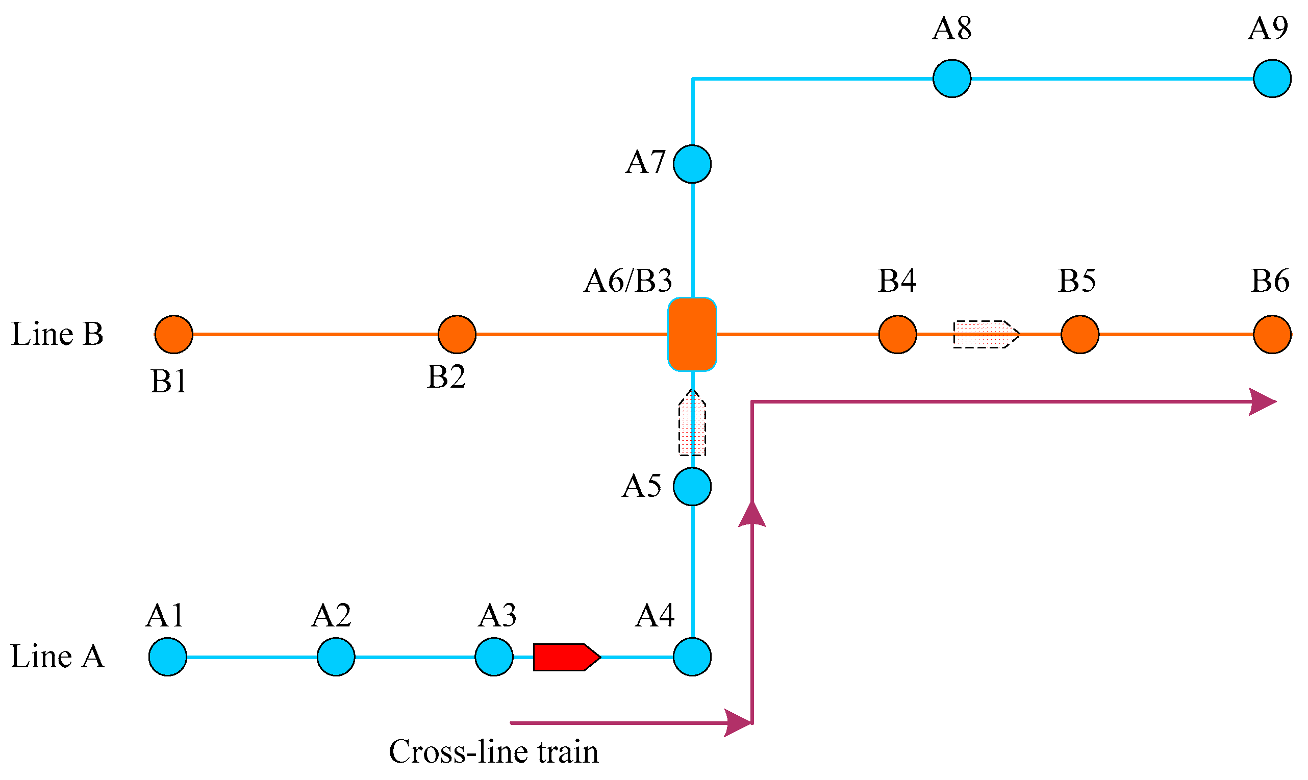
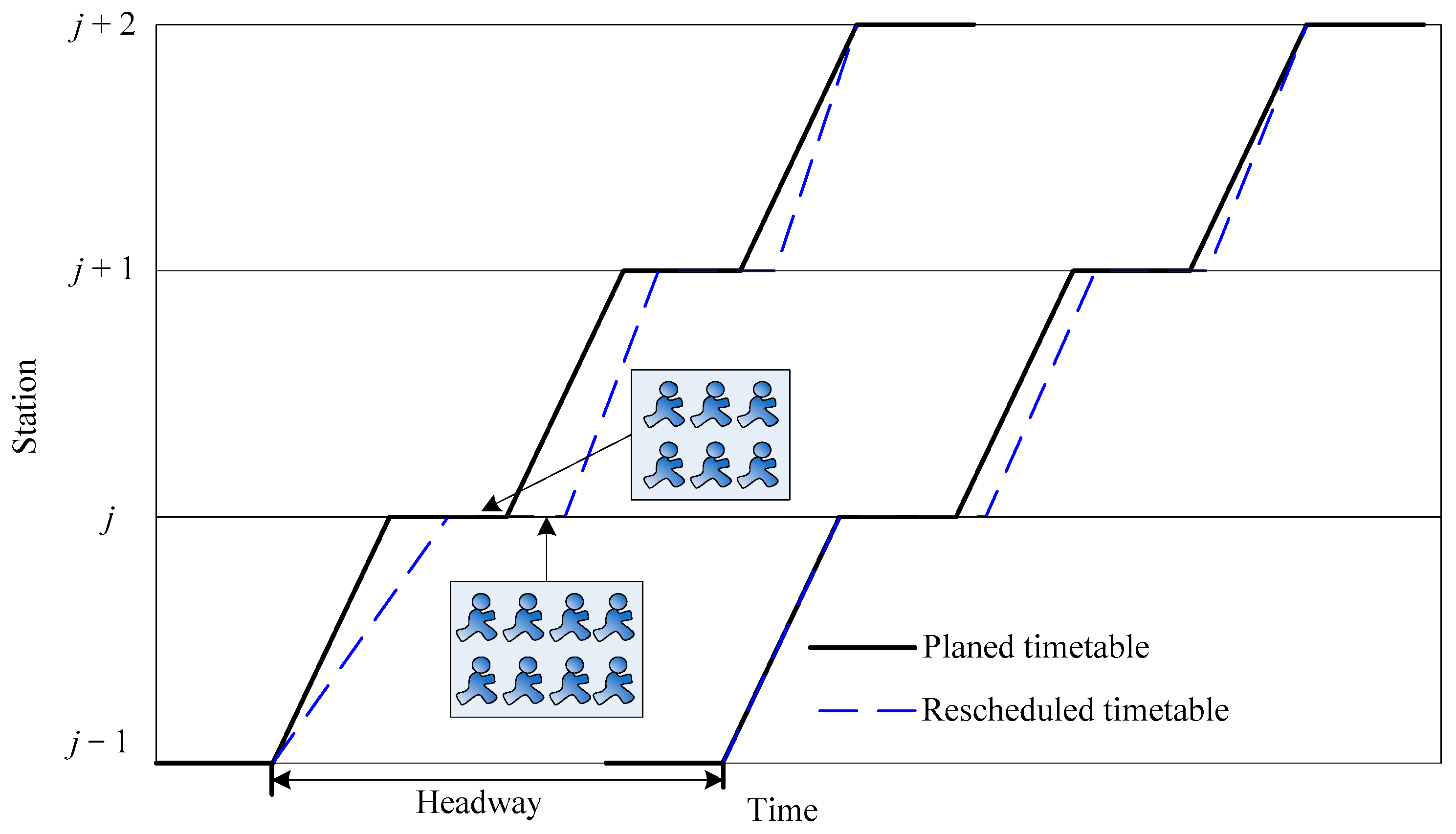
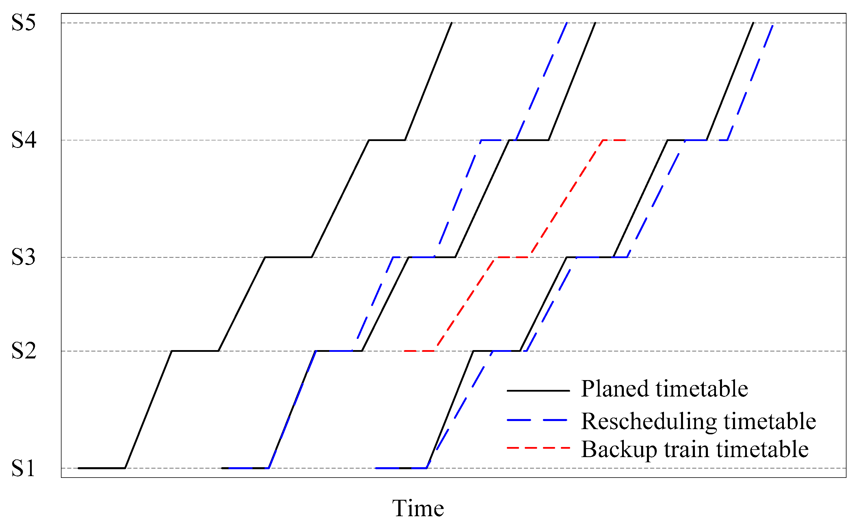
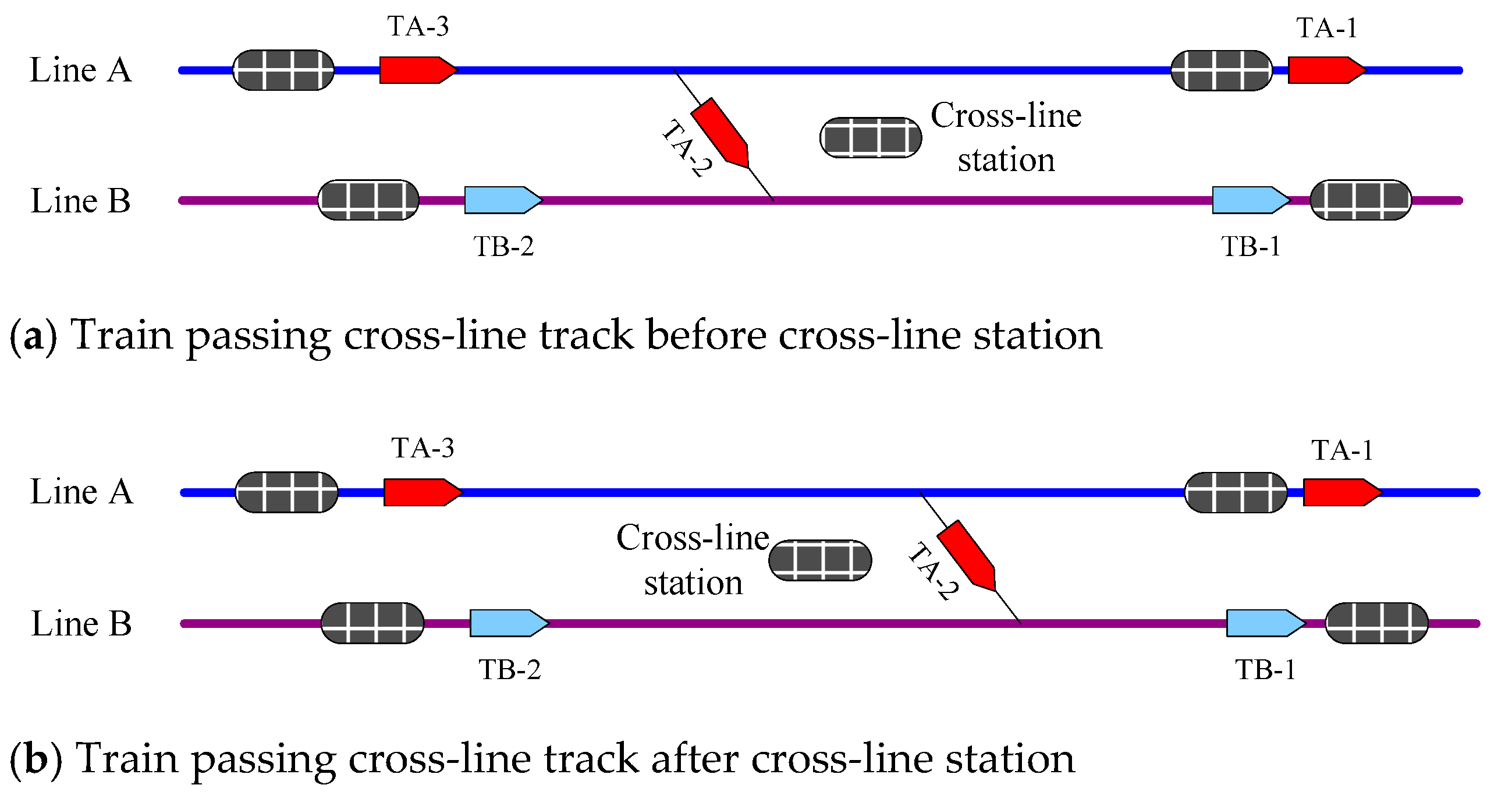
2. Problem Description

In the context of networked operation, the coupling between lines makes passenger flow management at interchange stations crucial [28,29,30]. The cross-line operation mode not only improves the travel experience of transfer passengers through cross-line trains, but also helps to serve emergency scenarios. For example, when a large number of passengers transferring out (i.e., a large passenger flow from a line to other lines via the interchange station) is suddenly detected on a line, a cross-line backup train can be added to alleviate the passenger flow. At the same time, when rescue trains are needed for adjacent lines, trains on the line can be used as cross-line trains. As shown in Figure 1, when an emergency occurs on Line B, trains (backup or mainline trains) of Line A can be used as rescue trains. At the same time, if a large transfer passenger flow from Line A to Line B suddenly occurs, it can also improve the service quality and alleviate the risk of passenger detain in the transfer station (i.e., station B3) by adding cross-line backup trains.

This paper focuses on train rescheduling strategies for large transfer passenger flow scenarios, involving two or more lines. As shown in Figure 1, to implement a cross-line service, Line A adds a cross-line train, and Line B also adds a temporary train service. The use of backup trains involves processes such as startup, arrival, departure, and return, thus it is necessary to optimize the schedule of the backup train and the planned trains by combining the routing of the backup train and the change of large passenger flow. This is because the train operation has strict safety constraints, each train needs to maintain a safe interval with its front and rear trains [31], and there is a significant coupling relationship between passenger flow and train flow, as shown in Figure 2 and Figure 3.

For the impact of adding backup trains on the train timetable, when the train operation interval is large enough, backup trains can be added without affecting other trains. When the train operation interval is small, the addition of backup trains will affect the operation of planned trains, as shown in Figure 3. At the same time, in addition to considering the impact of adding cross-line backup train on the train timetable, it is also necessary to consider the online timing, the train routing, and the passenger flow evacuation effect for providing a complete scheme and quantitative decision-making basis for the cross-line train in emergency scenarios. Specifically, the problem considered in this paper is how to coordinate and optimize the operation plans of trains on the origin line (i.e., the origin line of the large transfer passenger flow), trains on the adjacent line, and the cross-line backup train in the early stages of large transfer passenger flow scenarios in order to better serve the transfer passengers and reduce the risk of passenger detain.

We use optimization theory to investigate the cooperative rescheduling problem of planned trains and the cross-line backup train. At the same time, while solving the problem, we discuss three hypotheses: (1) the operation trajectory of the cross-line backup train has an impact on the number of transfer passengers served by the backup train; (2) the number of transfer passengers served by the backup train will be limited when the deviation of the planned timetable or the running efficiency of the backup train is limited; (3) when the passenger flow is large enough, whether passenger data is taken into account has a limited impact on the number of transfer passengers served by the backup train. It should be noted that the analysis of these hypotheses is based on the proposed optimization models and the experiment data.

2.1. Basic Assumptions

Urban rail transit lines usually have two directions, the up-direction and the down-direction. For the convenience of research, only one direction is considered, and the opposite direction can be operated according to the same principle. Meanwhile, we set the following reasonable assumptions:

Assumption 1:

The train running sequence and the train routings in the planned timetable remain unchanged, and there is no “skip-stop” operation;

Assumption 2:

The passenger flow data is known, including the destination rates of passenger flows arriving at different stations;

Assumption 3:

For the large transfer passenger flow scenario, one backup train is enough as an emergency cross-line train;

Assumption 4:

The scenario involves two lines with the interoperability condition between them.

2.2. Symbol Definition

For ease of description, Line A represents the origin line of a large transfer passenger flow, and Line B represents the target line of the flow. Meanwhile, we define the following sets, parameters, and variables.

Set:

$N^A$/$N^B$: Set of trains in the planned timetable of Line A/Line B, and index is $i$;

$S^A$/$S^B$: Set of stations at Line A/Line B, and index is $j$ and $k$;

$S_i$: Set of stations that train $i$ passes through on Line A or Line B;

$\left\{l\right\}$: Set of cross-line backup trains, including train $l$;

$S_l^A/S_l^B$: Set of stations that train $l$ passes through on Line A/Line B;

$T$: Set of time units, and index is $m$.

Parameter:

$A_{i,j}$/$D_{i,j}$: The planned arrival/departure time of train $i$ at station $j$;

$r_{j-1,j}^{\min \_\mathrm{A}}$/$r_{j-1,j}^{\min \_\mathrm{B}}$: The minimum running time between station $j$ and $j-1$ on Line A/Line B;

$I_a^h$/$I_b^h$: The minimum tracking interval time for train operation on Line A/Line B;

$I_a^p$/$I_b^p$: The minimum departure-arrival interval for train operation on Line A/Line B;

$I_b^{front}$: The minimum interval between train $l$ and its preceding train at the cross-line station;

$I_b^{back}$: The minimum interval between train $l$ and its following train at the cross-line station;

$w_j^{\min \_\mathrm{A}}$/$w_j^{\min \_\mathrm{B}}$: The minimum dwelling time of trains at station $j$ of Line A/Line B;

$w^o$: The additional dwelling time provided by train $l$ for non-transfer passengers to alight at the previous station of the cross-line station;

$T^{\min \_\mathrm{dev}}$: The minimum deviation value of the planned timetables for Line A and B due to the addition of the cross-line backup train;

${\epsilon }^{di}$: The deviation tolerance coefficient of the planned timetables, and the larger the tolerance coefficient, the smaller the limit on the degree of deviation;

${\psi }_{di}$: Adjustment step for the deviation tolerance coefficient of the planned timetables;

$T^{\min \_\mathrm{r}}$: The fastest time for train $l$ to reach the cross-line station;

${\epsilon }^{ef}$: The running efficiency tolerance coefficient set for train $l$;

${\psi }_{ef}$: Adjustment step for the running efficiency tolerance coefficient of train $l$;

$t_m$: The mth timestamp;

$o_{j,m}$: The number of passengers arriving at station $j$ in the mth time unit;

$p_{k,j}$: The proportion of passengers boarding at station $k$ with the purpose of station $j$;

$q_j$: The proportion of passengers transferring out to the corresponding direction of Line B in the passengers who boarding at station $j$ of Line A with cross-line stations as their target stations for transferring out or exiting.

$L_{\max }$: The maximum passenger capacity of a train;

$\mathrm{M}$: A reasonably large number.

Decision variable:

$a_{i,j}$/$d_{i,j}$: The arrival/departure time of train $i$ at station $j$;

$a_{l,j}$/$d_{l,j}$: The arrival/departure time of train $l$ at station $j$;

$z_{l,i-1}^a$/$z_{l,i-1}^b$: The decision variable of whether train $l$ is located after train $i$ − 1 and before train $i$ when it is on Line A/Line B.

Intermediate variable:

$v_{i,j}^r$: The number of stranded passengers when train departs from station $j$;

$v_{i,j}^{add}$: The number of new arrivals at station $j$ within the interval $d_{i,j-1}$ to $d_{i,j}$;

$v_{l,j}^{add}$: The number of new arrivals at station $j$ during the period when train $l$ and its preceding train leave the station successively;

$L_{i,j}^n$: The number of passengers boarding train $i$ at station $j$;

$L_{i,j}^f$: The number of passengers alighting from train $i$ at station $j$;

$L_{i,j}^c$: The number of passengers on train $i$ when it arrives at station $j$;

$L_{i,j}^{n1}$: The number of passengers boarding train $i$ when the demand for station $j$ is relatively low;

$L_{i,j}^{n2}$: The number of passengers boarding train $i$ when the demand for station $j$ is relatively high;

$L_{l,j}^{n1}$,$L_{l,j}^{n2}$: Variables set for the calculation of $L_{l,j}^n$;

${\lambda }_{i,j,m}$: The Boolean variable set for comparing the departure time $d_{i,j}$ and timestamp $t_m$;

${\lambda }_{l,j,m}^c$: The Boolean variable set for comparing the departure time $d_{l,j}$ and timestamp $t_m$;

$y_{i,j}$,$y_{l,j}$: The Boolean variable that plays an auxiliary role for model transformation;

$b_{i,j}^a$,$b_{i,j}^d$: Auxiliary variables for model transformation.

3. Mathematical Model

3.1. Constraints

(1)

Constraints related to train operation

In terms of the operation interval, we consider the tracking interval and the departure-arrival interval. For the planned trains on Line A, they need to meet the following constraints:

$$a_{i,j}-a_{i-1,j}\ge I_a^h, i,i-1\in N^A, j\in S^A.$$

(1)

$$d_{i,j}-d_{i-1,j}\ge I_a^h, i,i-1\in N^A, j\in S^A.$$

(2)

$$a_{i,j}-d_{i-1,j}\ge I_a^p, i,i-1\in N^A, j\in S^A.$$

(3)

At the same time, the planned trains on Line B also need to consider the operation interval; therefore, we obtain:

$$a_{i,j}-a_{i-1,j}\ge I_b^h, i,i-1\in N^B,j\in S^B.$$

(4)

$$d_{i,j}-d_{i-1,j}\ge I_b^h, i,i-1\in N^B,j\in S^B.$$

(5)

$$a_{i,j}-d_{i-1,j}\ge I_b^p, i,i-1\in N^B,j\in S^B.$$

(6)

The cross-line backup train also requires consideration of the operation interval, which means that the tracking interval and the departure-arrival interval between the backup train and the planned train should meet the corresponding safety requirements. Specifically, for $i,i-1\in N^A$, $j\in S_l^A$, if cross-line backup train $l$ is located after train $i-1$, before train $i$ (i.e., between train $i-1$ and train $i$, and $z_{l,i-1}^a=1$), we obtain:

$$a_{l,j}-a_{i-1,j}\ge I_a^h.$$

(7)

$$a_{i,j}-a_{l,j}\ge I_a^h.$$

(8)

$$d_{l,j}-d_{i-1,j}\ge I_a^h.$$

(9)

$$d_{i,j}-d_{l,j}\ge I_a^h.$$

(10)

$$a_{l,j}-d_{i-1,j}\ge I_a^p.$$

(11)

$$a_{i,j}-d_{l,j}\ge I_a^p.$$

(12)

Similarly, for $i,i-1\in N^B$,$j\in S_l^B$, when cross-line backup train $l$ is located between train $i-1$ and train $i$ (i.e., $z_{l,i-1}^b=1$), we obtain:

$$a_{l,j}-a_{i-1,j}\ge I_b^h.$$

(13)

$$a_{i,j}-a_{l,j}\ge I_b^h.$$

(14)

$$d_{l,j}-d_{i-1,j}\ge I_b^h.$$

(15)

$$d_{i,j}-d_{l,j}\ge I_b^h.$$

(16)

$$a_{l,j}-d_{i-1,j}\ge I_b^p.$$

(17)

$$a_{i,j}-d_{l,j}\ge I_b^p.$$

(18)

In terms of dwelling time, when a planned train on Line A and Line B is operating normally, its dwelling time should not be less than the corresponding minimum dwelling time; therefore, we obtain:

$$d_{i,j}-a_{i,j}\ge w_j^{\min \_\mathrm{A}}, i\in N^A, j\in S_{}^A.$$

(19)

$$d_{i,j}-a_{i,j}\ge w_j^{\min \_\mathrm{B}}, i\in N^B, j\in S_{}^B.$$

(20)

Similarly, when adding a cross-line backup train to operate on Line A, its dwelling time should meet the corresponding constraints. However, the backup train needs to consider the additional dwelling time at the previous station of the cross-line station to provide convenience for other passengers not going to Line B. At this point, we obtain:

$$d_{l,j}-a_{l,j}\ge w_j^{\min \_\mathrm{A}}+\mathrm{sign}\left(j,\max \left(S_l^A\right)\right)\times w^o, j\in S_l^A.$$

(21)

where $\mathrm{sign}\left(j,\max \left(S_l^A\right)\right)$ is used to indicate whether $j$ is equal to $\max \left(S_l^A\right)$. If $j=\max \left(S_l^A\right)$, the symbol is equal to 1, otherwise 0.

The cross-line backup train should also meet the dwelling time constraint when running on Line B; therefore, we obtain:

$$d_{l,j}-a_{l,j}\ge w_j^{\min \_\mathrm{B}}, j\in S_l^B.$$

(22)

In terms of train running time in a section, when adjusting the panned timetables of Lines A and B, it is necessary to consider the train running time in different sections, and the constraints are formulated as follows:

$$a_{i,j}-d_{i,j-1}\ge r_{j-1,j}^{\min \_\mathrm{A}}, i\in N^A, j,j-1\in S_{}^A.$$

(23)

$$a_{i,j}-d_{i,j-1}\ge r_{j-1,j}^{\min \_\mathrm{B}}, i\in N^B, j,j-1\in S_{}^B.$$

(24)

For the operation of the cross-line backup train on Line A and Line B, the running time in different sections should also meet the corresponding constraints:

$$a_{l,j}-d_{l,j-1}\ge r_{j-1,j}^{\min \_\mathrm{A}}, j\in S_l^A.$$

(25)

$$a_{l,j}-d_{l,j-1}\ge r_{j-1,j}^{\min \_\mathrm{B}}, j\in S_l^B.$$

(26)

Meanwhile, the cross-line backup train may cause the actual train timetable to deviate from the planned timetable, and operators do not want the timetable to deviate too much. To address this, we have the following constraint [32]:

$${\displaystyle \sum _{i\in \left\{N^A,N^B\right\},j\in S_i}\left|a_{i,j}-A_{i,j}\right|+{\displaystyle \sum _{i\in \left\{N^A,N^B\right\},j\in S_i}\left|d_{i,j}-D_{i,j}\right|}}\le (1+{\epsilon }^{di})\times T^{\min \_\mathrm{dev}}.$$

(27)

For emergency scenarios, the high-efficiency operation of the backup train may be a good strategy, but it will affect the operation of other trains and cause a large timetable deviation. Then, we also have the following constraint [22]:

$$a_{l,\min (S_l^B)}\le (1+{\epsilon }^{ef})\times T^{\min \_\mathrm{r}}.$$

(28)

In terms of the utilization of the backup train, when adopting the strategy of adding a cross-line backup train to cope with an emergency, it is necessary to ensure that the train is arranged between the planned trains on Lines A and B; therefore, we obtain:

$${\displaystyle \sum _{i-1\in N^A}{z}_{l,i-1}^a}=1.$$

(29)

$${\displaystyle \sum _{i-1\in N^B}{z}_{l,i-1}^b}=1.$$

(30)

Since the time for the backup train to arrive at the station of Line A should not be less than the expected time, the following constraints should be considered:

$$a_{l,\min (S_l^A)}\ge A_{l,\min (S_l^A)}^e.$$

(31)

In terms of the operation interval at the cross-line station, as shown in Figure 4, passing the cross-line track before the station (i.e., Figure 4a) and passing the cross-line track after the station (i.e., Figure 4b) are the cross-line forms of a cross-line train. To ensure the safe and orderly connection between the cross-line train and the planned train on Line B at the cross-line station, it is necessary to meet the safety interval requirements between the cross-line train and its previous and rear trains.

Taking Figure 4 as an example, Train TA-2 is a cross-line train running from Line A to Line B. According to the safety interval requirements, the train TA-2 and its front and rear trains TB-1 and TB-2 on Line B should, respectively, meet the following conditions [33]:

$$\begin{array}{l}{d}_{\mathrm{TA}-2,j}-d_{\mathrm{TB}-1,j}\ge \max (I_b^h,I_b^{front})\\ d_{\mathrm{TB}-2,j}-d_{\mathrm{TA}-2,j}\ge \max (I_b^h,I_b^{back})\end{array}.$$

Generally, if the cross-line backup train $l$ is located between train $i-1$ and train $i$ on Line B (i.e., $z_{l,i-1}^b=1$), then for $j=\min (S_l^b)$, we obtain:

$$d_{l,j}-d_{i-1,j}\ge \max (I_b^h,I_b^{front}).$$

(32)

$$d_{i,j}-d_{l,j}\ge \max (I_b^h,I_b^{back}).$$

(33)

(2)

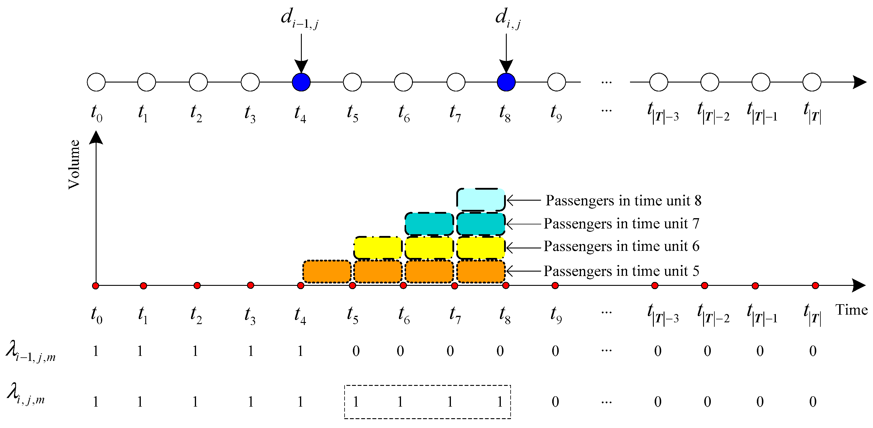
Constraints related to passenger flow calculation

In terms of new passenger volume, this paper considers the dynamic characteristics of passenger flow arriving at platforms. Specifically, for Line A, the research period $\left[t_{start},t_{end}\right]$ is divided into a series of time units based on the time-indexed method, and a set of time units $T$ is formed, involving time stamps $\{t_0,t_1,t_2,t_3,t_4,\cdots ,t_{\left|T\right|-2},t_{\left|T\right|-1},t_{\left|T\right|}\}$, where $t_{start}=t_0$, $t_{end}=t_{\left|T\right|}$. Further combined with the arrival data of passengers on the Line, a dynamic passenger flow matrix $De$ can be set.

$$De=\left[\begin{array}{cccccc}{o}_{1,1}& o_{1,2}& o_{1,3}& \cdots & o_{1,\left|T\right|-1}& o_{1,\left|T\right|}\\ o_{2,1}& o_{2,2}& o_{2,3}& \cdots & o_{2,\left|T\right|-1}& o_{2,\left|T\right|}\\ o_{3,1}& o_{3,2}& o_{3,3}& \cdots & o_{3,\left|T\right|-1}& o_{3,\left|T\right|}\\ ⋮& ⋮& ⋮& \cdots & ⋮& ⋮\\ o_{\left|S^A\right|-1,1}& o_{\left|S^A\right|-1,2}& o_{\left|S^A\right|-1,3}& \cdots & o_{\left|S^A\right|-1,\left|T\right|-1}& o_{\left|S^A\right|-1,\left|T\right|}\\ o_{\left|S^A\right|,1}& o_{\left|S^A\right|,2}& o_{\left|S^A\right|,3}& \cdots & o_{\left|S^A\right|,\left|T\right|-1}& o_{\left|S^A\right|,\left|T\right|}\end{array}\right].$$

(34)

Furthermore, for the coupling between the passenger flow and trains, the Boolean variable ${\lambda }_{i,j,m}$ is introduced to characterize the relationship between the departure time $d_{i,j}$ and each timestamp. It is specified that if $d_{i,j}$ is not less than the timestamp $t_m$, ${\lambda }_{i,j,m}$ is equal to 1, otherwise, 0. Then, we obtain:

$${\lambda }_{i,j,m}=\left\{\begin{array}{cc}1& d_{i,j}\ge t_m\\ 0& d_{i,j}<t_m\end{array}\right., i\in N^A, j\in S_{}^A, m\in T.$$

(35)

Similarly, the Boolean variable ${\lambda }_{i,j,m}$ is further introduced to characterize the relationship between the departure time $d_{l,j}$ of the train $l$ on Line A at station $j$ and timestamps; therefore, we obtain:

$${\lambda }_{l,j,m}^c=\left\{\begin{array}{cc}1& d_{l,j}\ge t_m\\ 0& d_{l,j}<t_m\end{array}\right., j\in S_l^A, m\in T.$$

(36)

Based on the above content, in terms of the newly arrived passenger volume within the departure interval of adjacent trains at the same station, for train $i$, the train ahead may or may not be the cross-line backup train. If the train ahead is not the cross-line backup train, the new demand is the number of passengers arriving during the departure of trains $i$ and $i-1$. There are two situations in which the train ahead is not the backup train for train $i$ at station $j$. One is that the backup train does not pass through station $j$, and the other is that the backup train passes through station $j$, but its sequence is not between train $i$ and $i-1$ (i.e., $z_{l,i-1}^a=0$). Combined with Figure 5, for $i,i-1\in N^A$, $j\in S_{}^A\backslash S_l^A$, we obtain:

$$v_{i,j}^{add}={\displaystyle \sum _{m=1}^{\left|T\right|}\left({\lambda }_{i,j,m}-{\lambda }_{i-1,j,m}\right)}\times o_{j,m}.$$

(37)

At the same time, if $z_{l,i-1}^a=0$, for $i,i-1\in N^A$, $j\in S_l^A$, we obtain:

$$v_{i,j}^{add}={\displaystyle \sum _{m=1}^{\left|T\right|}\left({\lambda }_{i,j,m}-{\lambda }_{i-1,j,m}\right)}\times o_{j,m}.$$

(38)

Otherwise, if $z_{l,i-1}^a=1$ and $j\in S_l^A$, for $i\in N^A$, we obtain:

$$v_{i,j}^{add}={\displaystyle \sum _{m=1}^{\left|T\right|}\left({\lambda }_{i,j,m}-{\lambda }_{l,j,m}^c\right)}\times o_{j,m}.$$

(39)

In terms of the cross-line backup train, the new demand also needs to be calculated in conjunction with timestamps and Boolean variables. For $j\in S_l^A$, $i,i-1\in N^A$, if $z_{l,i-1}^a=1$, we obtain:

$$v_{l,j}^{add}={\displaystyle \sum _{m=1}^{\left|T\right|}\left({\lambda }_{l,j,m}^c-{\lambda }_{i-1,j,m}\right)}\times o_{j,m}.$$

(40)

In terms of the number of stranded passengers, due to the cross-line backup train, it is necessary to consider whether the train in front of train $i$ at station $j$ is the backup train. Similar to the constraints of new passenger volume, we obtain:

$$v_{i,j}^r=v_{i-1,j}^r+v_{i,j}^{add}-L_{i,j}^n, i,i-1\in N^A, j\in S_{}^A\backslash S_l^A.$$

(41)

At the same time, if $z_{l,i-1}^a=0$, for $i,i-1\in N^A$, $j\in S_l^A$, we obtain:

$$v_{i,j}^r=v_{i-1,j}^r+v_{i,j}^{add}-L_{i,j}^n.$$

(42)

And for $j\in S_l^A$, if $z_{l,i-1}^a=1$, then we obtain:

$$v_{i,j}^r=v_{l,j}^r+v_{i,j}^{add}-L_{i,j}^n.$$

(43)

For the cross-line backup train $l$, the number of stranded passengers $v_{i,j}^r$ when it leaves station $j$ is also the number of stranded passengers when the previous train leaves the station, plus the number of passengers arriving within the time interval between it and the previous train leaving the station, minus the number of passengers boarding train $l$ at the station. Thus, for $i-1\in N^A$, $j\in S_l^A$, if $z_{l,i-1}^a=1$, we obtain:

$$v_{l,j}^r=v_{i-1,j}^r+v_{l,j}^{add}-L_{l,j}^n.$$

(44)

In terms of the number of alighting passengers, for different trains at station $j$, the OD (i.e., original and destination) distribution probability matrix $\mathbf{P}$ is first defined.

$$\mathbf{P}=\left[\begin{array}{cccccc}0& p_{1,2}& p_{1,3}& \cdots & p_{1,\left|\mathrm{S}\right|-1}& p_{1,\left|\mathrm{S}\right|}\\ 0& 0& p_{2,3}& \cdots & p_{2,\left|S\right|-1}& p_{2,\left|\mathrm{S}\right|}\\ 0& 0& 0& \cdots & p_{3,\left|\mathrm{S}\right|-1}& p_{3,\left|\mathrm{S}\right|}\\ ⋮& ⋮& ⋮& \cdots & ⋮& ⋮\\ 0& 0& 0& \cdots & 0& p_{\left|\mathrm{S}\right|-1,\left|\mathrm{S}\right|}\\ 0& 0& 0& \cdots & 0& 0\end{array}\right].$$

(45)

Furthermore, according to the OD distribution probability matrix, the number of alighting passengers from train $i$ at station $j$ is

$$L_{i,j}^f={\displaystyle \sum _{k=1}^j\left(p_{k,j}\times L_{i,k}^n\right)}, i\in N^A, j\in S_{}^A.$$

(46)

For the backup train, considering that some passengers do not travel to Line B, the number of alighting passengers at station $j$ is

$$L_{l,j}^f=\left\{\begin{array}{l}{\displaystyle \sum _{k=\min (S_l^A)}^j\left(p_{k,j}\times L_{l,k}^n\right)}, j\in S_l^A\backslash \left\{\max \left(S_l^A\right)\right\}\\ {\displaystyle \sum _{j^{\prime }=\max \left(S_l^A\right)}^{\left|S_{}^A\right|}{\displaystyle \sum _{k=\min (S_l^A)}^j\left(p_{k,j^{\prime }}\times L_{l,k}^n\right)}}, j=\max \left(S_l^A\right)\end{array}\right..$$

(47)

In terms of the number of passengers in train $i$, when it arrives at the first station, the number of passengers in the train is 0. When it arrives at other stations, the number of passengers in the train is the number of passengers in the train when it arrives at the previous station plus the number of passengers getting on at the previous station, and minus the number of passengers getting off at the previous station. Then, for $i\in N^A$, we obtain:

$$L_{i,j}^c=\left\{\begin{array}{cc}0\hfill & j=1\hfill \\ L_{i,j-1}^c+L_{i,j-1}^n-L_{i,j-1}^f\hfill & j\in S_i^A\backslash \left\{1\right\}\hfill \end{array}\right..$$

(48)

Similarly, for the backup train, the corresponding constraint is:

$$L_{l,j}^c=\left\{\begin{array}{cc}0\hfill & j=\min (S_l^A)\hfill \\ L_{l,j-1}^c+L_{l,j-1}^n-L_{l,j-1}^f\hfill & j\in S_l^A\backslash \left\{\min (S_l^A)\right\}\hfill \end{array}\right..$$

(49)

The number of passengers boarding train $i$ at station $j$ needs to be explored based on different situations. When the current demand is low and the remaining capacity is sufficient, the demand can all enter the train. The demand includes the number of stranded passengers from the previous train and the new demand. Due to the possibility that the previous train may be the planned train $i-1$ or the cross-line backup train $l$, we obtain:

$$L_{i,j}^{n1}=v_{i-1,j}^r+v_{i,j}^{add}, i,i-1\in N^A, j\in S_{}^A\backslash S_l^A.$$

(50)

At the same time, for $i,i-1\in N^A$, $j\in S_l^A$ and $z_{l,i-1}^a=0$, we also obtain:

$$L_{i,j}^{n1}=v_{i-1,j}^r+v_{i,j}^{add}.$$

(51)

In addition, for $i\in N^A$, $j\in S_l^A$, if $z_{l,i-1}^a=1$, we obtain:

$$L_{i,j}^{n1}=v_{l,j}^r+v_{i,j}^{add}.$$

(52)

When there is a high demand and the remaining capacity cannot meet the demand, the number of passengers boarding the train is the remaining capacity of the train. Then, we obtain:

$$L_{i,j}^{n2}=L_{\max }-L_{i,j}^c+L_{i,j}^f, i,i-1\in N^A, j\in S_{}^A.$$

(53)

Based on the relationship between demand and remaining capacity, the number of passengers boarding train $i$ at station $j$ can be further expressed as

$$L_{i,j}^n=\min \left(L_{i,j}^{n1},L_{i,j}^{n2}\right), i\in N^A, j\in S_{}^A.$$

(54)

Meanwhile, for the backup train $l$, if the front train is train $i-1$ and the current demand is low and the remaining capacity is sufficient, the current demand can all enter the train. Thus, for $i,i-1\in N^A$,$j\in S_l^A$, if $z_{l,i-1}^a=1$, we obtain:

$$L_{l,j}^{n1}=v_{i-1,j}^r+v_{l,j}^{add}.$$

(55)

If the demand is larger than the remaining capacity, the number of passengers boarding train $l$ is the remaining capacity of the train. Thus, we obtain:

$$L_{l,j}^{n2}=L_{\max }-L_{l,j}^c+L_{l,j}^f, j\in S_l^A.$$

(56)

Similarly, based on the relationship between demand and capacity, the number of passengers boarding train $l$ at station $j$ can be expressed as

$$L_{l,j}^n=\min \left(L_{l,j}^{n1},L_{l,j}^{n2}\right), j\in S_l^A.$$

(57)

3.2. Objective Function

This paper focuses on optimizing the rescheduled timetable related to a cross-line service in response to large transfer passenger flow scenarios. Due to the constraints that already include the running efficiency of the cross-line backup train and the degree of deviation from the planned timetable, the optimization objective is to maximize the number of transfer passengers served by the cross-line backup train, which are calculated by

$$\min f=-{\displaystyle \sum _{j\in S_l^A}\left(p_{j,\max (S_l^A)}\times q_j\times L_{l,j}^n\right)}.$$

(58)

Based on the above constraints and the objective function, the optimization model shown in Equation (59) can be obtained (Model I, for short):

$$\begin{array}{c}\min f=-{\displaystyle \sum _{j\in S_l^A}\left(p_{j,\max (S_l^A)}\times q_j\times L_{l,j}^n\right)}\hfill \\ s.t.\left\{\begin{array}{l}\mathrm{Constraints} (1)–(33),(35)–(44),(46)–(57)\\ a_{i,j},d_{i,j}\in R^{+}, \forall i\in \left\{N^A,N^B\right\},j\in S_i\\ a_{l,j},d_{l,j}\in R^{+}, \forall j\in S_l\\ z_{l,i-1}^a,z_{l,i-1}^b\in \left\{0,1\right\}, \forall i-1\in \left\{N^A,N^B\right\}\end{array}\right.\hfill \end{array}.$$

(59)

4. Model Transformation and Solution Approaches

For Model I, constraints (7)–(18), (32), (33), (35), (36), (38)–(40), (42)–(44), (51)–(52), and (55) are typical IF-THEN nonlinear terms, constraint (27) contains an absolute value term, and constraints (54) and (57) also contain the MIN term. Therefore, Model I is a nonlinear model. If it is solved by a normal solver, it needs to be transformed. Meanwhile, due to the large number of variables in the model, it is necessary to consider a suitable solution approach.

4.1. Model Transformation

For model transformation, we propose the following lemmas using the large m method, formula derivations, auxiliary variables, and auxiliary constraints.

Lemma 1.

For $i,i-1\in N^A$, $j\in S_l^A$, constraints (7)–(12) can be transformed into the linear form shown in Equation (60) [22]:

$$\left\{\begin{array}{l}{a}_{l,j}-a_{i-1,j}\ge I_a^h-(1-z_{l,i-1}^a)\times \mathrm{M}\\ a_{i,j}-a_{l,j}\ge I_a^h-(1-z_{l,i-1}^a)\times \mathrm{M}\\ d_{l,j}-d_{i-1,j}\ge I_a^h-(1-z_{l,i-1}^a)\times \mathrm{M}\\ d_{i,j}-d_{l,j}\ge I_a^h-(1-z_{l,i-1}^a)\times \mathrm{M}\\ a_{l,j}-d_{i-1,j}\ge I_a^p-(1-z_{l,i-1}^a)\times \mathrm{M}\\ a_{i,j}-d_{l,j}\ge I_a^p-(1-z_{l,i-1}^a)\times \mathrm{M}\\ z_{l,i-1}^a\in \left\{0,1\right\}\end{array}\right..$$

(60)

Lemma 2.

For $i,i-1\in N^B$, $j\in S_l^B$, constraints (13)–(18) can be transformed into the linear form shown in Equation (61) [22]:

$$\left\{\begin{array}{l}{a}_{l,j}-a_{i-1,j}\ge I_b^h-(1-z_{l,i-1}^b)\times \mathrm{M}\\ a_{i,j}-a_{l,j}\ge I_b^h-(1-z_{l,i-1}^b)\times \mathrm{M}\\ d_{l,j}-d_{i-1,j}\ge I_b^h-(1-z_{l,i-1}^b)\times \mathrm{M}\\ d_{i,j}-d_{l,j}\ge I_b^h-(1-z_{l,i-1}^b)\times \mathrm{M}\\ a_{l,j}-d_{i-1,j}\ge I_b^p-(1-z_{l,i-1}^b)\times \mathrm{M}\\ a_{i,j}-d_{l,j}\ge I_b^p-(1-z_{l,i-1}^b)\times \mathrm{M}\\ z_{l,i-1}^b\in \left\{0,1\right\}\end{array}\right..$$

(61)

Lemma 3.

For $i\in \left\{N^A,N^B\right\}$, $j\in S_i$, constraint (27) can be transformed into the linear form shown in Equation (62):

$$\left\{\begin{array}{l}{\displaystyle \sum _{i,j}\left(b_{i,j}^a+b_{i,j}^d\right)}\le (1+\gamma )\times T^{\min \_\mathrm{dev}}\\ A_{i,j}-a_{i,j}\le b_{i,j}^a\\ a_{i,j}-A_{i,j}\le b_{i,j}^a\\ D_{i,j}-d_{i,j}\le b_{i,j}^d\\ d_{i,j}-D_{i,j}\le b_{i,j}^d\\ a_{i,j},d_{i,j},b_{i,j}^a,b_{i,j}^d\in Z^{+}\end{array}\right..$$

(62)

where $b_{i,j}^a$ and $b_{i,j}^d$ are auxiliary variables. Combining the minimization feature of the objective function (Equation (58), conditions $A_{i,j}-a_{i,j}\le b_{i,j}^a$ and $a_{i,j}-A_{i,j}\le b_{i,j}^a$ make $b_{i,j}^a$ equal to $\left|a_{i,j}-A_{i,j}\right|$ [34,35], and constraints $D_{i,j}-d_{i,j}\le b_{i,j}^d$ and $d_{i,j}-D_{i,j}\le b_{i,j}^d$ make $b_{i,j}^d$ equal to $\left|d_{i,j}-D_{i,j}\right|$.

Lemma 4.

For $i,i-1\in N^B$, $j=\min (S_l^b)$, constraints (32) and (33) can be transformed into the linear form, as shown in Equation (63) [22]:

$$\left\{\begin{array}{l}{d}_{l,j}-d_{i-1,j}\ge \max (I_b^h,I_b^{front})-(1-z_{l,i-1}^b)\times \mathrm{M}\\ d_{i,j}-d_{l,j}\ge \max (I_b^h,I_b^{back})-(1-z_{l,i-1}^b)\times \mathrm{M}\\ z_{l,i-1}^b\in \left\{0,1\right\}\end{array}\right..$$

(63)

Lemma 5.

For $j\in S_l^A$, $m\in T$, constraints (35) and (36) can be transformed into the linear form, as shown in Equation (64) [34]:

$$\left\{\begin{array}{l}{t}_m-d_{l,j}\le \mathrm{M}\times (1-{\lambda }_{l,j,m}^c)\\ d_{l,j}-t_m\le \mathrm{M}\times {\lambda }_{l,j,m}^c-1\\ t_m-d_{i,j}\le \mathrm{M}\times (1-{\lambda }_{i,j,m})\\ d_{i,j}-t_m\le \mathrm{M}\times {\lambda }_{i,j,m}-1\\ {\lambda }_{l,j,m}^c\in \{0,1\}\\ {\lambda }_{i,j,m}\in \left\{0,1\right\}\end{array}\right..$$

(64)

Lemma 6.

For $i,i-1\in N^A$, $j\in S_l^A$, $m\in T$, constraints (38) and (39) can be transformed into the linear form, as shown in Equation (65):

$$v_{i,j}^{add}= {\displaystyle \sum _{m=1}^{\left|T\right|}\left({\lambda }_{i,j,m}-{\lambda }_{i-1,j,m}\right)}\times o_{j,m}-{\displaystyle \sum _{m=1}^{\left|T\right|}\left({\lambda }_{l,j,m}^c\times z_{l,i-1}^a-{\lambda }_{i-1,j,m}\times z_{l,i-1}^a\right)\times o_{j,m}},$$

(65)

where the meaning of constraints (37) and (38) is: for $i,i-1\in N^A$, $j\in S_l^A$, if $z_{l,i-1}^a=0$, then $v_{i,j}^{add}={\displaystyle \sum _{m=1}^{\left|T\right|}\left({\lambda }_{i,j,m}-{\lambda }_{i-1,j,m}\right)}\times o_{j,m}$, and if $z_{l,i-1}^a=1$, then $v_{i,j}^{add}={\displaystyle \sum _{m=1}^{\left|T\right|}\left({\lambda }_{i,j,m}-{\lambda }_{l,j,m}^c\right)}\times o_{j,m}$. Based on this, we obtain:

$$\begin{array}{cc}\hfill v_{i,j}^{add}& =\left(1-z_{l,i-1}^a\right)\times {\displaystyle \sum _{m=1}^{\left|T\right|}\left({\lambda }_{i,j,m}-{\lambda }_{i-1,j,m}\right)}\times o_{j,m}+z_{l,i-1}^a\times {\displaystyle \sum _{m=1}^{\left|T\right|}\left({\lambda }_{i,j,m}-{\lambda }_{l,j,m}^c\right)}\times o_{j,m}\hfill \\ & ={\displaystyle \sum _{m=1}^{\left|T\right|}\left({\lambda }_{i,j,m}-{\lambda }_{i-1,j,m}\right)}\times o_{j,m}-{\displaystyle \sum _{m=1}^{\left|T\right|}\left({\lambda }_{i,j,m}-{\lambda }_{i-1,j,m}\right)}\times z_{l,i-1}^a\times o_{j,m}+{\displaystyle \sum _{m=1}^{\left|T\right|}\left({\lambda }_{i,j,m}-{\lambda }_{l,j,m}^c\right)}\times z_{l,i-1}^a\times o_{j,m}\hfill \\ & ={\displaystyle \sum _{m=1}^{\left|T\right|}\left({\lambda }_{i,j,m}-{\lambda }_{i-1,j,m}\right)}\times o_{j,m}-z_{l,i-1}^a\times \left[{\displaystyle \sum _{m=1}^{\left|T\right|}\left({\lambda }_{i,j,m}-{\lambda }_{i-1,j,m}\right)}\times o_{j,m}-{\displaystyle \sum _{m=1}^{\left|T\right|}\left({\lambda }_{i,j,m}-{\lambda }_{l,j,m}^c\right)}\times o_{j,m}\right]\hfill \\ & ={\displaystyle \sum _{m=1}^{\left|T\right|}\left({\lambda }_{i,j,m}-{\lambda }_{i-1,j,m}\right)}\times o_{j,m}-z_{l,i-1}^a\times {\displaystyle \sum _{m=1}^{\left|T\right|}\left({\lambda }_{l,j,m}^c-{\lambda }_{i-1,j,m}\right)}\times o_{j,m}\hfill \\ & ={\displaystyle \sum _{m=1}^{\left|T\right|}\left({\lambda }_{i,j,m}-{\lambda }_{i-1,j,m}\right)}\times o_{j,m}-{\displaystyle \sum _{m=1}^{\left|T\right|}\left({\lambda }_{l,j,m}^c\times z_{l,i-1}^a\times o_{j,m}-{\lambda }_{i-1,j,m}\times z_{l,i-1}^a\times o_{j,m}\right)}\hfill \\ & ={\displaystyle \sum _{m=1}^{\left|T\right|}\left({\lambda }_{i,j,m}-{\lambda }_{i-1,j,m}\right)}\times o_{j,m}-{\displaystyle \sum _{m=1}^{\left|T\right|}\left({\lambda }_{l,j,m}^c\times z_{l,i-1}^a-{\lambda }_{i-1,j,m}\times z_{l,i-1}^a\right)\times o_{j,m}}\hfill \end{array}.$$

Lemma 7.

For $i,i-1\in N^A$, $j\in S_l^A$, constraint (40) can be transformed into the linear form, as shown in Equation (66) [22]:

$$\left\{\begin{array}{l}{v}_{l,j}^{add}\le \left(1-z_{l,i-1}^a\right)\times \mathrm{M}+{\displaystyle \sum _{m=1}^{\left|T\right|}\left({\lambda }_{l,j,m}^c-{\lambda }_{i-1,j,m}\right)}\times o_{j,m}\\ v_{l,j}^{add}\ge {\displaystyle \sum _{m=1}^{\left|T\right|}\left({\lambda }_{l,j,m}^c-{\lambda }_{i-1,j,m}\right)}\times o_{j,m}-\left(1-z_{l,i-1}^a\right)\times \mathrm{M}\end{array}\right..$$

(66)

Lemma 8.

For $i,i-1\in N^A$, $j\in S_l^A$, constraints (42) and (43) can be transformed into the linear form, as shown in Equation (67):

$$v_{i,j}^r=\left(v_{i-1,j}^r+v_{i,j}^{add}-L_{i,j}^n\right)+z_{l,i-1}^a\times \left(v_{l,j}^r-v_{i-1,j}^r\right),$$

(67)

where the meanings of constraints (42) and (43) are: For $i,i-1\in N^A$, $j\in S_l^A$, if $z_{l,i-1}^a=0$, then $v_{i,j}^r=v_{i-1,j}^r+v_{i,j}^{add}-L_{i,j}^n$, and if $z_{l,i-1}^a=1$, then $v_{i,j}^r=v_{l,j}^r+v_{i,j}^{add}-L_{i,j}^n$. Based on this, we obtain:

$$\begin{array}{cc}\hfill v_{i,j}^r& =\left(1-z_{l,i-1}^a\right)\times \left(v_{i-1,j}^r+v_{i,j}^{add}-L_{i,j}^n\right)+z_{l,i-1}^a\times \left(v_{l,j}^r+v_{i,j}^{add}-L_{i,j}^n\right)\hfill \\ & =\left(v_{i-1,j}^r+v_{i,j}^{add}-L_{i,j}^n\right)-z_{l,i-1}^a\times v_{i-1,j}^r+z_{l,i-1}^a\times v_{l,j}^r\hfill \\ & =\left(v_{i-1,j}^r+v_{i,j}^{add}-L_{i,j}^n\right)+z_{l,i-1}^a\times \left(v_{l,j}^r-v_{i-1,j}^r\right)\hfill \end{array}.$$

Lemma 9.

For $i,i-1\in N^A$, $j\in S_l^A$, constraint (44) can be transformed into the linear form, as shown in Equation (68) [22]:

$$\left\{\begin{array}{l}{v}_{l,j}^r\le \left(1-z_{l,i-1}^a\right)\times \mathrm{M}+v_{i-1,j}^r+v_{l,j}^{add}-L_{l,j}^n\\ v_{l,j}^r\ge v_{i-1,j}^r+v_{l,j}^{add}-L_{l,j}^n-\left(1-z_{l,i-1}^a\right)\times \mathrm{M}\end{array}\right..$$

(68)

Lemma 10.

For $i,i-1\in N^A$, $j\in S_l^A$, the constraints (51) and (52) can be transformed into the linear form, as shown in Equation (69):

$$L_{i,j}^{n1} =\left(v_{i-1,j}^r+v_{i,j}^{add}\right)+z_{l,i-1}^a\times \left(v_{l,j}^r-v_{i-1,j}^r\right),$$

(69)

where, the meanings of constraints (51) and (52) are: For $i,i-1\in N^A$, $j\in S_l^A$, if $z_{l,i-1}^a=0$, then $L_{i,j}^{n1}=v_{i-1,j}^r+v_{i,j}^{add}$, and if $z_{l,i-1}^a=1$, then $L_{i,j}^{n1}=v_{l,j}^r+v_{i,j}^{add}$. Based on this, we obtain:

$$\begin{array}{cc}\hfill L_{i,j}^{n1}& =\left(1-z_{l,i-1}^a\right)\times \left(v_{i-1,j}^r+v_{i,j}^{add}\right)+z_{l,i-1}^a\times \left(v_{l,j}^r+v_{i,j}^{add}\right)\hfill \\ & =\left(v_{i-1,j}^r+v_{i,j}^{add}\right)-z_{l,i-1}^a\times \left(v_{i-1,j}^r+v_{i,j}^{add}\right)+z_{l,i-1}^a\times \left(v_{l,j}^r+v_{i,j}^{add}\right)\hfill \\ & =\left(v_{i-1,j}^r+v_{i,j}^{add}\right)-z_{l,i-1}^a\times v_{i-1,j}^r+z_{l,i-1}^a\times v_{l,j}^r\hfill \\ & =\left(v_{i-1,j}^r+v_{i,j}^{add}\right)+z_{l,i-1}^a\times \left(v_{l,j}^r-v_{i-1,j}^r\right)\hfill \end{array}.$$

Lemma 11.

For $i\in N^A$, $j\in S_{}^A$, constraint (54) can be transformed into the linear form, as shown in Equation (70):

$$\left\{\begin{array}{l}{L}_{i,j}^n\ge L_{i,j}^{n1}-\mathrm{M}\times (1-y_{i,j})\\ L_{i,j}^n\ge L_{i,j}^{n2}-\mathrm{M}\times y_{i,j}\\ L_{i,j}^n\le L_{i,j}^{n1}\\ L_{i,j}^n\le L_{i,j}^{n2}\\ y_{i,j}\in \{0,1\}\end{array}\right.,$$

(70)

where $y_{i,j}$ is the auxiliary variable. If $L_{i,j}^{n1}$ is less than $L_{i,j}^{n2}$, then $y_{i,j}$ is equal to 1, $L_{i,j}^n=L_{i,j}^{n1}$. If $L_{i,j}^{n1}$ is greater than $L_{i,j}^{n2}$, then $y_{i,j}$ is equal to 0, $L_{i,j}^n=L_{i,j}^{n2}$. If $L_{i,j}^{n1}$ equals $L_{i,j}^{n2}$, then $y_{i,j}$ equals 1 or 0.

Lemma 12.

For $i,i-1\in N^A$, $j\in S_l^A$, constraint (55) can be transformed into the linear form, as shown in Equation (71) [22]:

$$\left\{\begin{array}{l}{L}_{l,j}^{n1}\le \left(1-z_{l,i-1}\right)\times \mathrm{M}+v_{i-1,j}^r+v_{l,j}^{add}\\ L_{l,j}^{n1}\ge v_{i-1,j}^r+v_{l,j}^{add}-\left(1-z_{l,i-1}\right)\times \mathrm{M}\end{array}\right..$$

(71)

Lemma 13.

For $j\in {\mathit{S}}_l^A$, constraint (57) can be transformed into the linear form, as shown in Equation (72):

$$\left\{\begin{array}{l}{L}_{l,j}^n\ge L_{l,j}^{n1}-\mathrm{M}\times (1-y_{l,j})\\ L_{l,j}^n\ge L_{l,j}^{n2}-\mathrm{M}\times y_{l,j}\\ L_{l,j}^n\le L_{l,j}^{n1}\\ L_{l,j}^n\le L_{l,j}^{n2}\\ y_{l,j}\in \{0,1\}\end{array}\right..$$

(72)

where  $y_{l,j}$ is the auxiliary variable, and the derivation of the lemma is consistent with Lemma 11.

Combining lemmas above, Model I can be further transformed into the form shown as Equation (73) (Model II, for short), which is a typical mixed integer programming (MIP) model with quadratic terms

$$\begin{array}{l}\min f=-{\displaystyle \sum _{j\in S_l^A}\left(p_{j,\max (S_l^A)}\times q_j\times L_{l,j}^n\right)}\\ s.t.\left\{\begin{array}{l}\mathrm{Constraints} (1)–(6),(19)–(26),(28)–(31)\\ \mathrm{Constraints} (37),(41),(46)–(50),(53),(56)\\ \mathrm{Constraints} (60)–(72)\\ z_{l,i-1}^a\in \left\{0,1\right\},\forall i,i-1\in N^A\\ z_{l,i-1}^b\in \left\{0,1\right\},\forall i,i-1\in N^B\\ a_{i,j},d_{i,j},b_{i,j}^a,b_{i,j}^d\in R^{+}, \forall i\in \left\{N^A,N^B\right\},j\in S_i\\ a_{l,j},d_{l,j}\in R^{+}, \forall j\in S_l\\ {\lambda }_{i,j,m}\in \left\{0,1\right\}, \forall i\in \left\{N^A,N^B\right\},j\in S_i,m\in T\\ {\lambda }_{l,j,m}^c\in \left\{0,1\right\},j\in S_l^A,m\in T\\ y_{i,j}\in \left\{0,1\right\},\forall i,i-1\in N^A,j\in S_{}^A\\ y_{l,j}\in \left\{0,1\right\},j\in S_l^A\end{array}\right.\end{array}.$$

(73)

4.2. Solution Approaches

After model transformation, Model II is a MIP model with quadratic terms, which can be solved by the Gurobi solver. Meanwhile, considering the large number of variables in the model and the emergency needs of large passenger flow scenarios, the following three solution approaches are designed:

(1)

Direct approach

As a baseline, the direct approach can be described as obtaining the optimal solution based on Model II using a solver. It is worth noting that the approach needs to first determine the key parameters in constraints (27) and (28), namely $T^{\min \_\mathrm{r}}$ and $T^{\min \_\mathrm{dev}}$. It is difficult to directly estimate the values of the two parameters. Combined with train operation-related constraints and constraints (27) and (28), a linear model (Model III, for short), as shown in Equation (74), is further constructed, which can also be solved by the Gurobi solver. After obtaining the values of parameters $T^{\min \_\mathrm{r}}$ and $T^{\min \_\mathrm{dev}}$, the relevant constraints in Model II can be updated and the model can be solved.

$$\begin{array}{l}\min f_1=\min \left[{\displaystyle \sum _{i\in \left\{N^A,N^B\right\},j\in S_i}\left(b_{i,j}^a+b_{i,j}^d\right)}+a_{l,\min (S_l^B)}\right]\\ s.t.\left\{\begin{array}{l}\mathrm{Constraints} (1)–(6),(19)–(26),(29)–(31)\\ \mathrm{Constraints} (60)–(63)\\ z_{l,i-1}^a\in \left\{0,1\right\}, \forall i,i-1\in N^A\\ z_{l,i-1}^b\in \left\{0,1\right\}, \forall i,i-1\in {\mathit{N}}^B\\ b_{i,j}^a,b_{i,j}^d,a_{i,j},d_{i,j}, \forall i\in \left\{{\mathbf{N}}^A,{\mathit{N}}^B\right\},j\in S_i\\ a_{l,j},d_{l,j}\in R^{+}, \forall j\in S_l\end{array}\right.\end{array}$$

(74)

(2)

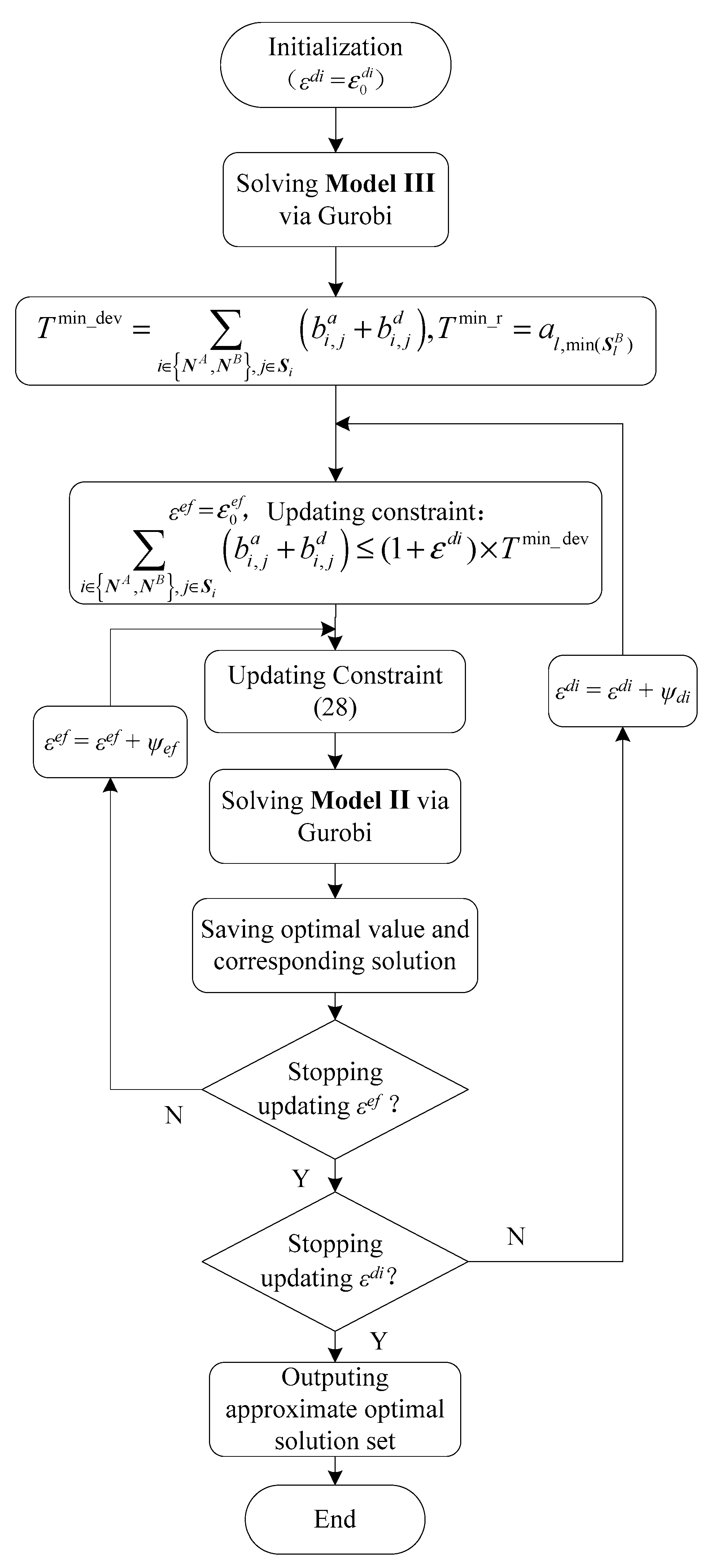
Dynamic adjustment approach

The dynamic adjustment approach can be expressed as dynamically adjusting the deviation tolerance coefficient of the planned timetables and the running efficiency tolerance coefficient of the cross-line backup train to obtain multiple groups of optimization schemes. For a complex model, obtaining an optimal solution can be very time consuming, and it may not need to search the optimal solution [36,37]. Meanwhile, when an emergency occurs, in addition to making quick decisions, decision-makers also expect to obtain multiple groups of emergency schemes for comparison and selection. In Model II, the values of the deviation tolerance coefficient and the running efficiency tolerance coefficient are related to decision-maker preference and may affect the magnitude of the objective function value. Based on this, this approach focuses on dynamically adjusting the two parameters, and introduces the adjustment step ${\psi }_{di}$ and ${\psi }_{ef}$ to design its flow. As shown in Figure 6, the approach achieves the goal of paying attention to the deviation degree of the planned timetable and increasing the emergency efficiency of the cross-line backup train while gradually iterating to obtain different emergency schemes.

In Figure 6, parameters $T^{\min \_\mathrm{r}}$ and $T^{\min \_\mathrm{dev}}$ are also calculated via the Gurobi solver first, and then the deviation tolerance coefficient of the planned timetable and the running efficiency tolerance coefficient of the cross-line backup train are dynamically adjusted. For the judgment conditions, the corresponding calculation time and the number of calculations can be required at a certain range. The outputted approximate Pareto optimal solution set can provide a reference for decision-makers [32], and can also be used to analyze the impact of relevant factors on the objective function value.

(3)

Emergency priority approach

The emergency priority approach can be described as obtaining an emergency scheme via the Gurobi solver based on Model III. Model III is a linear model that can be solved to obtain a rescheduled timetable, but the timetable does not consider passenger flow characteristics.

In summary, the three solution approaches correspond to different optimization models. Specifically, the first solution approach (i.e., the direct approach) corresponds to Model II, and in order to obtain an exact solution of Model II, its parameters are fixed. The corresponding result is a train rescheduling scheme considering the dynamic characteristics of passenger flow. The second solution approach (i.e., the dynamic adjustment approach) corresponds to Model II and Model III, and some parameters of Model II are dynamically adjusted, which is to obtain multiple effective solutions of Model II. The corresponding results are train rescheduling schemes, taking into account the dynamic characteristics of passenger flow, as well as different tolerances of the timetable deviation and the backup train’s running efficiency. The third solution approach (i.e., the emergency priority approach), corresponding to Model III, is to obtain an exact solution of Model III, and the corresponding result is a train rescheduling scheme without considering passenger flow data.

5. Computational Experiments

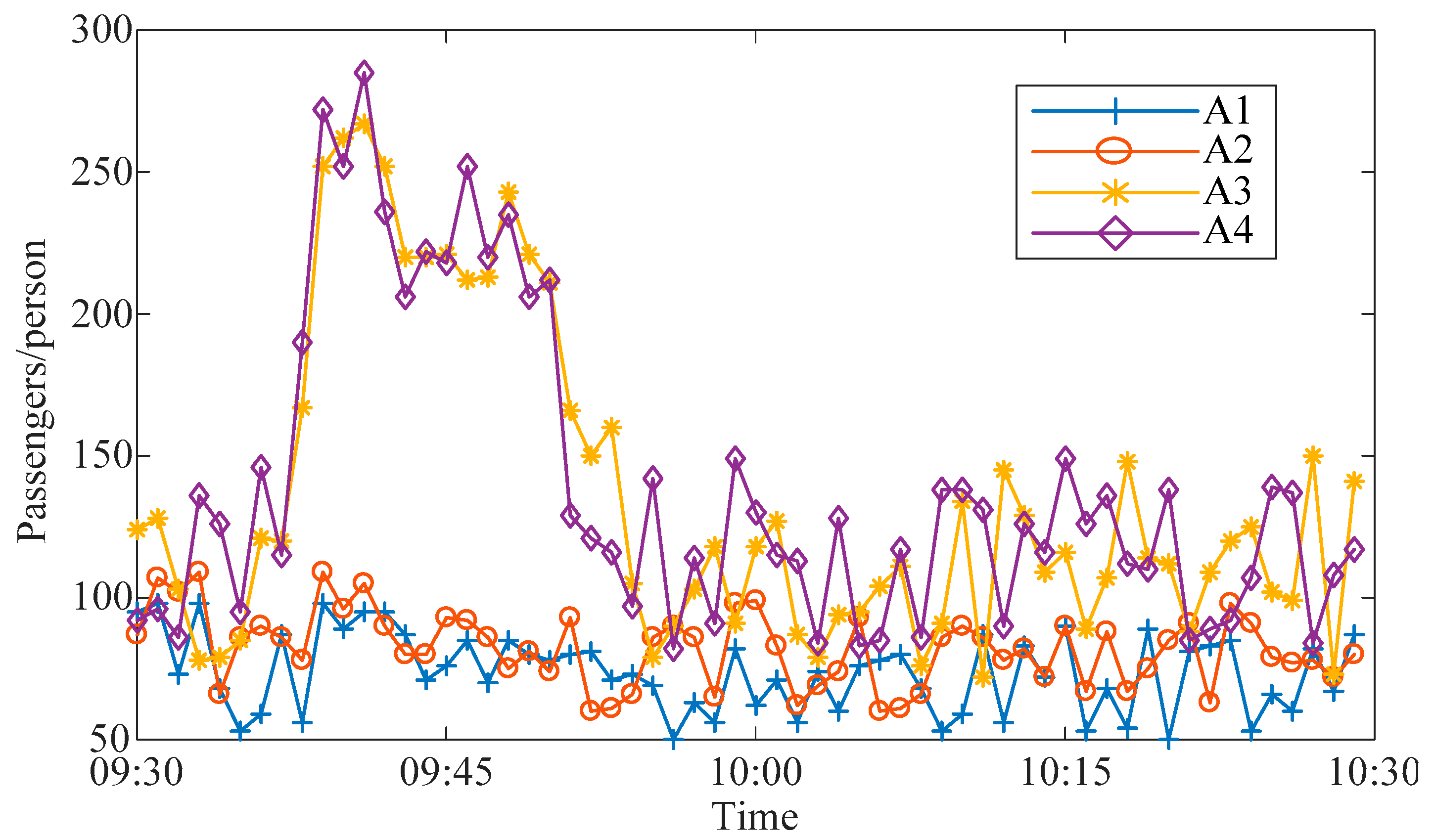
5.1. Experiment Description

As shown in Figure 7, the basic data of the two lines (Line A and Line B, for short) are from reference [38], and the lines are the planned lines of Chongqing Rail Transit in China, including the corresponding train organization scheme [38]. Line A has 15 stations numbered A1 to A15. Line B has 11 stations numbered B1 to B11. Stations A5 and B3 have the conditions for cross-line operation. We assume that at 09:40, stations A3 and A4 detect a large passenger flow for Line B, the main direction of the large passenger flow on Line B is B1 to B11. To ensure the operational safety of stations A3 and A4, as well as interchange station A5 or B3, and improve the quality of passenger service, it has been decided to temporarily add a cross-line service. The initial station of the cross-line backup train is A3, and the train passes the cross-line track before station A5 (i.e., the routing of the train is A3, A4, B3, B4, …, and B11).

For parameters, we set the values of each parameter according to the parameter values in reference [38] and the problem background. Specifically, the planned intervals for Line A and Line B are 150 s and 180 s, respectively, the minimum tracking interval is 120 s, and the minimum departure-arrival interval is 90 s. Meanwhile, the planned dwelling time and minimum dwelling time (s) for stations A1 to A15 are {35, 30, 30, 30, 35, 30, 30, 30, 30, 30, 35, 30, 30, 30, 35} and {30, 25, 25, 25, 30, 25, 25, 25, 25, 25, 25, 25, 30, 30, 25, 25, 30}, respectively, The planned running time and minimum running time (s) of the sections, are {150, 180, 153, 153, 117, 162, 180, 198, 135, 240, 162, 180, 198} and {120, 144, 122, 122, 93, 93, 129, 144, 158, 108, 192, 129, 144, 158}, respectively. The planned dwelling time and minimum dwelling time (s) for stations B1 to B11 are {35, 30, 35, 30, 30, 30, 30, 35, 35, 30, 30, 35} and {30, 25, 30, 25, 25, 25, 30, 25, 25, 30}, respectively. The planned running time and minimum running time (s) for the sections are {207, 180, 162, 135, 108, 135, 135, 162, 180, 198, 207} and {165, 144, 129, 108, 86, 108, 129, 144, 158, 165}, respectively [38].

The matrix of destination rate for the passenger flow on Line A is shown in

Table 1. Destination rate for passenger flow.

Station	A2	A3	A4	A5	A6	A7	A8	A9	A10	A11	A12	A13	A14	A15
A1	0.034	0.034	0.037	0.332	0.044	0.047	0.050	0.052	0.055	0.058	0.062	0.063	0.065	0.067
A2	--	0.015	0.013	0.615	0.024	0.026	0.030	0.033	0.036	0.039	0.029	0.045	0.048	0.047
A3	--	--	0.008	0.816	0.011	0.013	0.014	0.016	0.017	0.019	0.021	0.022	0.020	0.023
A4	--	--	--	0.725	0.018	0.020	0.023	0.025	0.028	0.030	0.033	0.033	0.034	0.031
A5	--	--	--	--	0.062	0.070	0.078	0.087	0.096	0.104	0.113	0.122	0.129	0.139
A6	--	--	--	--	--	0.065	0.073	0.082	0.089	0.097	0.124	0.141	0.156	0.173
A7	--	--	--	--	--	--	0.073	0.081	0.089	0.097	0.132	0.154	0.176	0.198
A8	--	--	--	--	--	--	--	0.088	0.097	0.105	0.139	0.164	0.191	0.216
A9	--	--	--	--	--	--	--	--	0.121	0.131	0.143	0.172	0.202	0.231
A10	--	--	--	--	--	--	--	--	--	0.221	0.147	0.179	0.211	0.242
A11	--	--	--	--	--	--	--	--	--	--	0.189	0.229	0.271	0.311
A12	--	--	--	--	--	--	--	--	--	--	--	0.283	0.334	0.383
A13	--	--	--	--	--	--	--	--	--	--	--	--	0.465	0.535
A14	--	--	--	--	--	--	--	--	--	--	--	--	--	1

. The data in the matrix is simulated data, which is used to verify the validity of the methods presented in this paper. In practice, the matrix can be calculated according to actual or predicted OD data in a certain direction [13]. For example, if 50 passengers get on trains in the direction at Station A13, 23 passengers go to Station A14, and 27 passengers go to Station A15 in a given period, the corresponding destination rates are 0.46 (i.e., 23/50) and 0.54 (i.e., 27/50). According to the utilization mode of the cross-line backup train, for the objective function of Model II, when analyzing the passenger flow data, it is only necessary to focus on the passenger flow on Line A. The dynamic arrival situation of the passenger flow at the platforms of stations A1 to A4 is shown in Figure 8, and among passengers boarding at stations A1, A2, A3, and A4 and aligning at stations A5 (i.e., the cross-line service is not taking into account), the proportion of passengers transferring to Line B is 0.42, 0.46, 0.78 and 0.86, respectively.

For simulation, Line A considers eight planned trains numbered Ta1 to Ta8, while Line B considers six planned trains numbered Tb1 to Tb8. The timetable of the first and last trains for the two lines is not adjusted, that is, the cross-line backup train is between them. The capacity of a train is set at 1320 people. The interval of the time unit for passenger flow calculation is taken as 60 s, and the larger number M is taken as 500,000. In addition, the version of the Gurobi solver is 9.1.0, and the computation termination condition is that the Gap is less than 0.1%.

Meanwhile, the first solution approach sets the deviation tolerance coefficient and the running efficiency tolerance coefficient to 20%. For the second solution approach, to observe the impact of the deviation tolerance coefficient and the running efficiency tolerance coefficient on the optimal value of the objective function, the initial values (${\epsilon }_0^{di}$ and ${\epsilon }_0^{ef}$) of the two are set to 0, and the adjustment step is set to 10%. In addition, to analyze whether the impact of the two parameters on the objective function value is related to demand, the passenger flow is amplified.

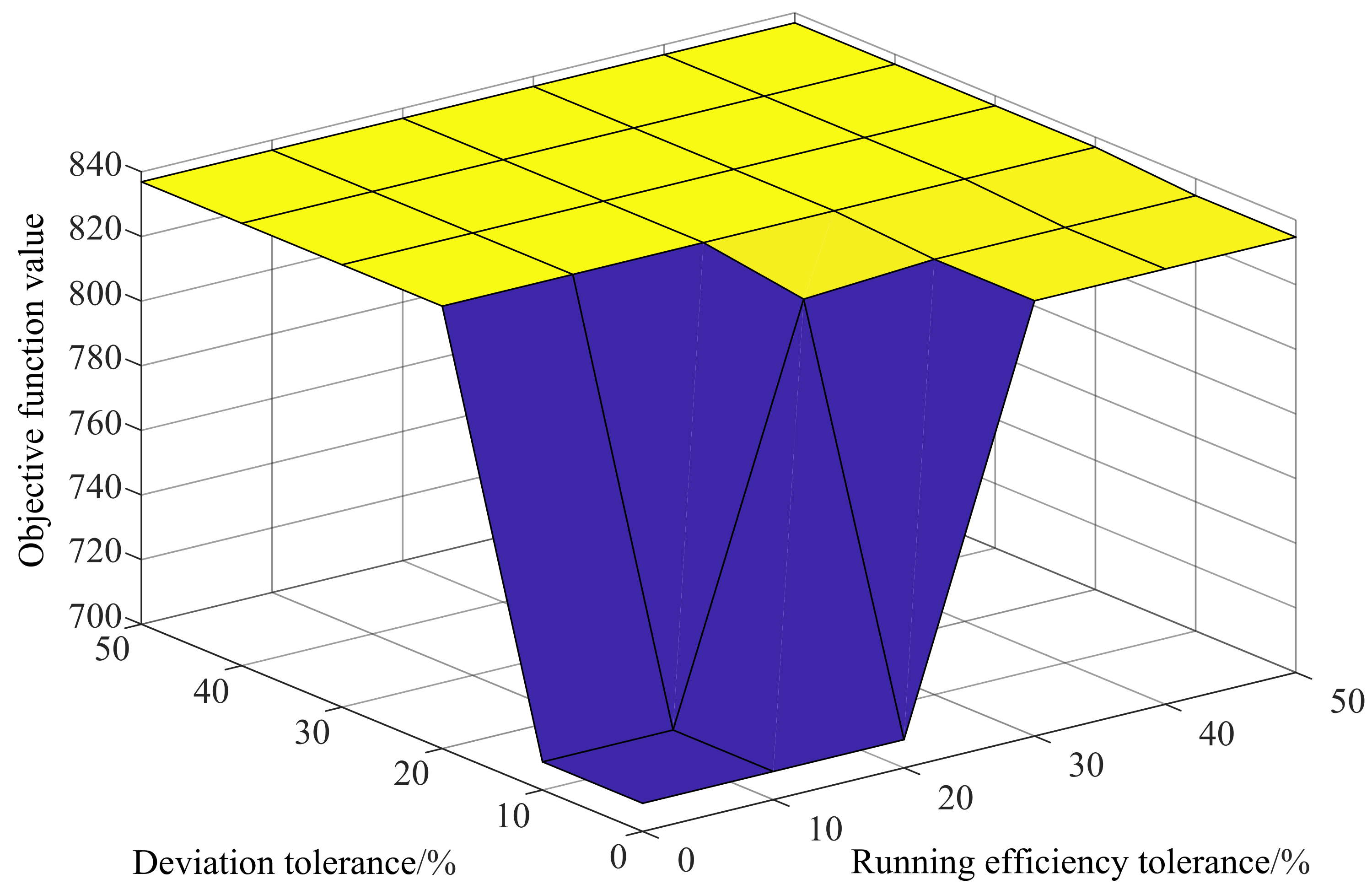
5.2. Results and Analysis

The optimal value of Model III obtained by the Gurobi solver is 3030 s, the values of parameters $T^{\min \_\mathrm{r}}$ and $T^{\min \_\mathrm{dev}}$ are 2024 s and 1006 s, respectively, the solving time is 0.177 s, and the corresponding Gap is 0%. The rescheduled timetable is shown in Figure 9, which can be used as the result of the third solution approach or the result of the second solution approach when the two tolerance coefficients are both 0. At the same time, following the process of the first solution approach, the values of the two parameters are substituted into Model II. The optimal value of Model II is 836.898, the solving time is 1.216 s, the Gap is 0%, and the rescheduled timetable is shown in Figure 10.

In Figure 9 and Figure 10, the cross-line backup train is located between the second and third planned trains (i.e., Ta2 and Ta3, and Tb2 and Tb3), but there are differences in arrival and departure times at different stations. In the two rescheduled timetable, both the previous train and the rear train of the backup train are affected, but neither has a significant deviation. It is worth noting that in the rescheduled timetable shown in Figure 9, the number of transfer passengers served by the cross-line backup train is 708, while for the rescheduled timetable shown in Figure 10, the corresponding value is 836.

Regarding the impact of the deviation tolerance and running efficiency tolerance on the objective function value, the results shown in Figure 11 are obtained based on the second solution approach. It can be intuitively observed that when the parameters are small, the objective function value is also small, and as the two increase synchronously, there is a trend of the objective function value increasing. For example, when both are taken as 0, the objective function value is 708.734; When both are taken as 30%, the objective function value is 836.898. According to Figure 11, for this experiment, the recommended adjustment range for the two coefficients in the second solution approach is [0, 30%].

After tripling the demand (i.e., passenger flow), a calculation is conducted by dynamically adjusting parameters according to the second solution approach, and it is found that the optimal values of the objective function are all 846.389. Meanwhile, the calculation result of the third solution approach is also 846.389. These results indicate that the larger demand reduces the impact of two parameters on the objective function value. When the demand is high, the number of passengers served by the train is also limited due to the limited capacity of the train, and the results obtained are consistent with the actual situation. Therefore, when in great demand, the rescheduled timetable for train operation can only be obtained based on Model III or the third solution approach.

To further analyze the advantages and disadvantages of the strategy of adding a cross-line backup service to the large transfer passenger flow, we compared it with the corresponding results of the original timetable. The relevant results of the two are shown in

Table 2. Results comparison for original timetable and rescheduled timetable.

Timetable	Transfer Passengers Served/Person	Remaining Capacity/Person 1	Transfer Passengers on Planned Trains/Person							Maximum Stranded Passengers/Person
			Ta2	Ta3	Ta4	Ta5	Ta6	Ta7	Ta8	A1	A2	A3	A4
Rescheduled timetable	836	484	556	476	605	438	483	440	428	0	0	0	170
Original timetable	--	--	556	669	558	596	556	550	428	0	0	0	1001

¹ The remaining capacity refers to the remaining capacity when the cross-line backup train arrives at station B3.

.

According to Table 2, it can be seen that in terms of the number of passengers transferring out at the interchange station (A5) for different planned trains, the maximum value of the rescheduled timetable is 605, the minimum value is 428, and the average value is 489. The maximum value of the original timetable is 669, the minimum value is 428, and the average value is 559. Therefore, the impact of the transfer passenger flow of each planned train in the rescheduled timetable on adjacent lines is relatively smaller. At the same time, the maximum number of stranded passengers obtained from the rescheduled timetable is also more ideal than the original timetable (e.g., Station A4, 170 < 1001). Furthermore, by adding a cross-line backup train, 836 passengers can transfer on the train, and a remaining capacity of 484 passengers is provided for the interchange station (i.e., B3), which helps improve the service quality and alleviate congestion at the station. It should be noted that adding a backup train increases operation costs, such as electricity consumption.

6. Discussion

In this section, we further discuss the validity of the proposed methods and the three hypotheses in Section 2. For the methods in this paper, the results verify the effectiveness of the models and solution approaches, which can provide theoretical references for large transfer passenger flow and emergency scenarios of cross-line operation. The optimization model focuses on evacuating passengers at the source line of large transfer passenger flow, considering the relevant conditions for train cross-line operation. For the scenarios involved, compared to the planned timetable, adopting the “adding a cross-line backup train” strategy can better ensure the operational safety of stations, including interchange stations, and improve service quality. The result accords with the expected effect of adding a backup train [12,19,20,21]. For solution approaches, the first and second can obtain effective solutions within seconds. For the first solution approach, it fixes the deviation tolerance and running efficiency tolerance, resulting in a relatively fixed solution. For the second solution approach, multiple sets of approximate optimal solutions can be obtained by dynamically adjusting the two parameters. In addition, the third solution approach can obtain a train rescheduling scheme without considering passenger flow data.

It should be noted that when adding a cross-line backup train, corresponding operating conditions are required, which involve cross-line operating conditions between lines, large operation intervals in the original timetable, and may have a certain impact on operating costs. In this regard, this paper assumes a suitable optimization premise, and in practice, emergency strategies can be adopted based on the characteristics of the scenarios. For example, when the cross-line operation condition is not available, strategies such as implementing passenger flow control on the source line of large transfer passenger flow or adding backup trains on the target line of large transfer passenger flow can also be adopted.

For the first of the three hypotheses discussed, the operation trajectories of the cross-line backup train in Figure 9 and Figure 10 are different, and the corresponding objective function values are also different. The result indicates that the arrival time and departure time of the cross-line backup train at each station have an impact on the number of transfer passengers served by the backup train. Therefore, when adding a backup train, it is necessary to determine its appropriate online time based on passenger flow data [21]. For the second hypothesis, Figure 11 obtained according to the second solution approach shows when the tolerance parameters of timetable deviation or backup train running efficiency are small, the objective function value is also small, and when the two parameters increase, the objective function value tends to increase, but this trend will disappear when the two parameters are large enough. The results show that the number of transfer passengers served by the backup train will be limited when limiting the tolerance coefficient of timetable deviation or backup train running efficiency. In fact, when the deviation of the planned timetable is limited or the running efficiency of the backup train is limited, the operation trajectory of the cross-line backup train is also limited, which is consistent with the characteristics of the first hypothesis. For the third hypothesis, when the initial demand in the experiment is amplified three times, the number of transfer passengers served by the backup train is the same when passenger flow data is considered and when passenger flow data is not considered. The result shows that when the passenger flow is large enough, the characteristics of the first hypothesis will be weakened and may even disappear. In fact, the result is consistent with common sense, which is related to the capacity of the train. When the demand is great, we can only focus on adjusting the timetable and directly calculate according to the third solution approach.

7. Conclusions

We conducted a study on how to better utilize a cross-line backup train to cope with a large transfer passenger flow. The train rescheduling model and solution approaches of adding the cross-line backup train and planned trains are studied to guide the emergency response in such scenarios. The experiments show that the mixed integer programming model is effective, and the solution efficiency is also high. The operation trajectory of the cross-line backup train has an impact on the objective function value, which is limited by the demand, the deviation tolerance of the planned timetable, and the running efficiency tolerance of the cross-line backup train. When the requirements for timetable deviation and running efficiency are reduced, the objective function value tends to increase. For example, when both are set at 30%, the number of transfer passengers served by the cross-line backup train is 836, which is an increase of 18.1% compared to when both are set at 0. After tripling the demand, the number of transfer passengers served remained stable at 846 and is not affected by changes in the two parameters. Choosing an appropriate tolerance coefficient for the demand situation is meaningful. When the demand does not exceed the service capacity, dynamically adjusting the two parameters to obtain multiple sets of rescheduled timetables is a suitable way to deal with such scenarios. When the demand exceeds the service capacity, we can only focus on the emergency efficiency of adding the cross-line backup train. For the cross-line service of transfer passengers, this study can provide a reference for train rescheduling in the context of networked operation and cross-line operation.

Regarding the possible directions for further research on the emergency scenario, we further suggest considering the details of the problem more finely. For example, operating costs can be considered as one of the optimization goals, as organizing a backup train requires a large amount of electricity consumption. At the same time, when the passenger flow is large, it can also be managed in combination with passenger flow control, especially as to whether it can achieve good operational control effects at a lower cost, including passenger flow organization and train organization. Furthermore, the operation of many trains usually follows a certain target speed profile, which determines the interval operation time and energy consumption. If the optimization of train organization can be carried out in conjunction with the target speed profile, more excellent results may be obtained.

References

1. Yang, A.; Wang, B.; Chen, Y.; Huang, J.; Xiong, J. Plan of Cross-line Train in Urban Rail Transit Based on the Capacity Influence. J. Transp. Syst. Eng. Inf. Technol. 2017, 17, 221–227. [Google Scholar]
2. Yang, A.; Wang, B.; Huang, J.; Li, C. Service Replanning in Urban Rail Transit Networks: Cross-line Express Trains for Reducing the Number of Passenger Transfers and Travel Time. Transp. Res. Part C 2020, 115, 102629. [Google Scholar] [CrossRef]
3. Chen, L.; Duan, X.; Bai, Y. Optimizing Cross-line Train Service Planning in Urban Rail Transit Network. Urban Rapid Rail Transit 2023, 36, 59–64. [Google Scholar]
4. Zeng, Q.; Peng, Q. Cross-Line Train Plan in Urban Rail Transit Considering the Multi-Group Train. J. Railw. Sci. Eng. 2023, 20, 878–889. [Google Scholar]
5. Huang, J.; Chen, Y.; Zhang, A.; Zhou, Q.; Bai, Y.; Mao, B. Optimization of Urban Rail Network Operation Scheme Considering Interconnection. J. Railw. Sci. Eng. 2023, 20, 1587–1597. [Google Scholar]
6. Zhen, Q.; Jing, S. Train Rescheduling Model with Train Delay and Passenger Impatience Time in Urban Subway Network. J. Adv. Transp. 2016, 50, 1990–2014. [Google Scholar] [CrossRef]
7. Chu, P.; Yu, Y.; Dong, D.; Yuan, J.; Chen, Y. Train Rescheduling for Urban Rail Transit Considering Replacement and Equilibrium. J. Wuhan Univ. Technol. Transp. Sci. Eng. 2022, 46, 389–393. [Google Scholar]
8. Gao, Y.; Kroon, L.; Schmidt, M.; Yang, L. Rescheduling A Metro Line in an Over-Crowded Situation after Disruptions. Transp. Res. Part B 2016, 93, 425–449. [Google Scholar] [CrossRef]
9. Wang, Y.; Zhao, K.; D’Ariano, A.; Niu, R.; Li, S.; Luan, X. Real-time Integrated Train Rescheduling and Rolling Stock Circulation Planning for a Metro Line Under Disruptions. Transp. Res. Part B 2021, 152, 87–117. [Google Scholar] [CrossRef]
10. Yin, J.; Yang, L.; D’Ariano, A.; Tang, T.; Gao, Z. Integrated Backup Rolling Stock Allocation and Timetable Rescheduling with Uncertain Time-variant Passenger Demand under Disruptive Events. Inf. J. Comput. 2022, 34, 3234–3258. [Google Scholar] [CrossRef]
11. Yoo, S.; Kim, H.; Kim, W.; Kim, N.; Lee, J. Controlling Passenger Flow to Mitigate the Effects of Platform Overcrowding on Train Dwell Time. J. Intell. Transp. Syst. 2022, 26, 366–381. [Google Scholar] [CrossRef]
12. Song, X.; Feng, X.; Wang, Z.; Huang, W.; Chen, M. Simulation Analysis of Large Inbound Passenger Flow Control Measures of Subway Station Based on Dynamic Path Planning. Transp. Stand. 2022, 8, 154–165. [Google Scholar]
13. Shi, J.; Yang, J.; Yang, L. Safety-oriented Cooperative Passenger Flow Control Model in Peak Hours for a Metro Line. J. Transp. Syst. Eng. Inf. Technol. 2019, 19, 125–131. [Google Scholar]
14. Li, Y.; He, J.; Peng, Z. Multi-station Passenger Flow Control Problem Considering Early Warning Mechanism and Operation Scheme. J. Railw. Sci. Eng. 2023, 20, 84–93. [Google Scholar]
15. Liu, R.; Li, S.; Yang, L. Collaborative Optimization for Metro Train Scheduling and Train Connections Combined with Passenger Flow Control Strategy. Omega 2020, 90, 101990. [Google Scholar] [CrossRef]
16. Shi, J.; Yang, L.; Yang, J.; Gao, Z. Service-oriented Train Timetabling with Collaborative Passenger Flow Control on an Oversaturated Metro Line: An Integer Linear Optimization Approach. Transp. Res. Part B 2018, 110, 26–59. [Google Scholar] [CrossRef]
17. Li, J.; Bai, Y.; Zhou, Y.; Chen, Z.; Xu, Q. Integrated Model on Inbound Passenger Flow Control and Timetable Regulation at Transfer Station. J. China Railw. Soc. 2020, 42, 9–18. [Google Scholar]
18. Yuan, Y.; Li, S.; Yang, L.; Gao, Z. Real-time Optimization of Train Regulation and Passenger Flow Control for Urban Rail Transit Network under Frequent Disturbances. Transp. Res. Part E 2022, 168, 102942. [Google Scholar] [CrossRef]
19. Ying, M. Shanghai World Expo and Metro Operation Assurance. Urban Mass Transit 2011, 14, 1–4. [Google Scholar]
20. Xiong, Y.; Wei, W. Application and Optimization of Urban Rail Transit Standby Train. Urban Mass Transit 2010, 13, 87–88. [Google Scholar]
21. Ye, M.; Qian, Z.; Li, J.; Cao, C. Selection and Optimization Model of Standby Train Deployment Stations on Urban Rail Transit for Large Passenger Flow. J. Traffic Transp. Eng. 2021, 21, 227–237. [Google Scholar]
22. Yin, J.; Wang, Y.; Tang, T.; Xun, J.; Su, S. Metro Train Rescheduling by Adding Backup Trains under Disrupted Scenarios. Front. Eng. Manag. 2017, 4, 418–427. [Google Scholar] [CrossRef]
23. Wang, Z.; Su, S.; Su, B.; Tang, T. A Metro Train Rescheduling Approach Considering Flexible Short-turning and Adding Backup Trains Strategies during Disruptions in the Case of the Vehicle Breakdown. In Proceedings of the 2021 IEEE International Intelligent Transportation Systems Conference, Indianapolis, IN, USA, 19–22 September 2021. [Google Scholar]
24. Wang, Z.; Zhang, X.; Chen, S.; Jian, M.; Chen, Z. A Metro Timetable Rescheduling Optimization Method in Case of Failure Train Rescue. J. Railw. Sci. Eng. 2023. [Google Scholar] [CrossRef]
25. Bai, G.; Guo, J.; Shi, H.; Yang, Y.; Zhang, T. Optimization for Transfer Coordination of Network Timetable in Urban Rail Transit. J. China Railw. Soc. 2016, 38, 1–7. [Google Scholar]
26. Sun, P.; Zhao, J.; Ding, H. The Optimization of Urban Rail Transit Operation Scheme Based on Coordinated Transfer. Railw. Transp. Econ. 2011, 33, 67–70. [Google Scholar]
27. Xu, R.; Liu, B.; Fan, W. Train Operation Adjustment Strategies in Metro Based on Transfer Capacity Coordination. J. Transp. Syst. Eng. Inf. Technol. 2017, 17, 164–170. [Google Scholar]
28. Yu, Y.; Chu, P.; Hong, H.; Yuan, J.; Zhao, H. Robustness Comparison of Shanghai Metro Networks from Line Interaction Perspective. Proc. SPIE 2022, 12081, 120812H. [Google Scholar]
29. Li, W.; Xu, R.; Zhu, W. Multi-line Cooperation Method for Passenger Flow Disposal in Metro Transfer Station under Train Delay. J. Tongji Univ. Nat. Sci. 2015, 43, 239–244. [Google Scholar]
30. Cui, X.; Lu, Q.; Xu, P.; Wang, Z.; Qin, H. Critical Station Identification Based on Node Importance Contribution Matrix in Urban Rail Transit Network. J. Railw. Sci. Eng. 2022, 19, 2524–2531. [Google Scholar]
31. Carvajal-Carreño, W.; Cucala, A.P.; Fernández-Cardador, A. Fuzzy Train Tracking Algorithm for the Energy Efficient Operation of CBTC Equipped Metro Lines. Eng. Appl. Artif. Intell. 2016, 53, 19–31. [Google Scholar] [CrossRef]
32. Xu, W.; Zhao, P.; Ning, L. A Practical Method for Timetable Rescheduling in Subway Networks during the End-of-Service Period. J. Adv. Transp. 2018, 2018, 5914276. [Google Scholar] [CrossRef]
33. Yang, X.; Hu, H.; Yang, S.; Wang, W.; Shi, Z.; Yu, H.; Huang, Y. Train Operation Adjustment Method of Cross-line Train in Urban Rail Transit Based on Coyote Optimization Algorithm. In Proceedings of the 2020 IEEE 23rd International Conference on Intelligent Transportation Systems (ITSC), Rhodes, Greece, 20–23 September 2020. [Google Scholar]
34. Wang, Y.; Zhu, S.; D’Ariano, A.; Yin, J.; Miao, J.; Meng, L. Energy-efficient Timetabling and Rolling Stock Circulation Planning Based on Automatic Train Operation Levels for Metro Lines. Transp. Res. Part C 2021, 129, 103209. [Google Scholar] [CrossRef]
35. Bemporad, A.; Morari, M. Control of Systems Integrating Logic, Dynamics, and Constraints. Automatica 1999, 35, 407–427. [Google Scholar] [CrossRef]
36. Baker, K.R. Computational Results for the Flowshop Tardiness Problem. Comput. Ind. Eng. 2013, 64, 812–816. [Google Scholar] [CrossRef]
37. Herrmann, F. Using Optimization Models for Scheduling in Enterprise Resource Planning Systems. Systems 2016, 4, 15. [Google Scholar] [CrossRef]
38. Tian, S. Study on Optimization of Train Routing Planning of Urban Rail Transit Considering Congestion Degree of Transfer Station; Beijing Jiaotong University: Beijing, China, 2019. [Google Scholar]
Figure 1. Schematic of train cross-line operation.
Applsci 13 11228 g001
Figure 2. Train operation interval and its coupling relationship with passenger flow.
Applsci 13 11228 g002
Figure 3. Impact of adding a backup train on timetable.
Applsci 13 11228 g003
Figure 4. Schematic of cross-line form for cross-line trains.
Applsci 13 11228 g004
Figure 5. Time labeling for calculating passenger flow.
Applsci 13 11228 g005
Figure 6. Solution process of dynamic adjustment approach.
Applsci 13 11228 g006
Figure 7. Schematic of simulated lines.
Applsci 13 11228 g007
Figure 8. Demand at stations before cross-line station on Line A.
Applsci 13 11228 g008
Figure 9. Train rescheduled timetable ( ε d i = 0, ε e f = 0).
Applsci 13 11228 g009
Figure 10. Train rescheduled timetable ( ε d i = 20%, ε e f = 20%).
Applsci 13 11228 g010
Figure 11. Impact of parameter changes on the objective function value.
Applsci 13 11228 g011