Abstract
Industrial processes involving manipulator robots require accurate positioning and orienting for high-quality results. Any decrease in positional accuracy can result in resource wastage. Machine learning methodologies have been proposed to analyze failures and wear in electronic and mechanical components, affecting positional accuracy. These methods are typically implemented in software for offline analysis. In this regard, this work proposes a methodology for detecting a positional deviation in the robot’s joints and its implementation in a digital system of proprietary design based on a field-programmable gate array (FPGA) equipped with several developed intellectual property cores (IPcores). The method implemented in FPGA consists of the analysis of current signals from a UR5 robot using discrete wavelet transform (DWT), statistical indicators, and a neural network classifier. IPcores are developed and tested with synthetic current signals, and their effectiveness is validated using a real robot dataset. The results show that the system can classify the synthetic robot signals for joints two and three with 97% accuracy and the real robot signals for joints five and six with 100% accuracy. This system aims to be a high-speed reconfigurable tool to help detect robot precision degradation and implement timely maintenance strategies.
1. Introduction
Robotic systems have revolutionized the manufacturing industry by providing unprecedented accuracy, precision, and speed. Accuracy is critical to ensure the robot can position and orient itself to the required locations and repeat the task over a long time with minimal error. One way to enhance the positioning accuracy of the robot is by focusing on the design stage. For instance, Kelaiaia et al. [1], present a comprehensive review of optimal design aspects for parallel manipulators and propose a methodology for achieving the optimal design of such manipulators. Additionally, improving robot performance indices can contribute to better accuracy. Brahmia et al. [2], propose a new dimensionless sensitivity index for Parallel Kinematic Manipulators (PKM), based on the definition of the local sensitivity index (LSI). This index aids in identifying the contribution of error sources to the positioning error of the manipulator for a given task. By reducing geometric errors in PKMs, this index can significantly enhance the positioning accuracy of the robot.
Despite their advanced capabilities, robots can still experience accuracy degradation due to several factors such as environmental conditions, assembly errors, manufacturing defects in the structure, backlash, and component wear [3]. Therefore, it is essential to monitor and maintain the accuracy of robotic systems to ensure optimal performance over time. Different factors involved in the positional degradation of industrial robots and failures caused by wear in electrical and mechanical components are frequently studied. In this regard, methods based on machine learning techniques have been proposed to identify failures, such as in [4] where the wavelet packet transform (WPT) and the hidden Markov model (HMM) are used to analyze acoustic emissions (EA) and identify failures in a rotate vector reducer (RV). A method based on artificial failure data, random forest regression (RFR), support vector regression (SVR), and deep neural network regression (DNNR) is proposed in [5] to identify overload anomalies in the robot’s end effector and their effect on the joints. Moreover, in [6], a simulation of the torque degradation of the actuator of an industrial robot is carried out, where it is determined that the robot controller cannot deal with failures of this type. Other works related to methodologies that deal with mechanical failures in robots can be consulted for gears [7,8,9,10] and RV [11].
Recent research on deep learning and fault detection techniques for robots includes several noteworthy works. In [12], the authors propose a method that combines a sparse auto-decoder with a support vector machine (SVM) to construct a fault detection model for the robot’s reducer. They utilize signals obtained from an attitude sensor composed of an accelerometer, gyroscope, and magnetometer. Another study, presented in [13], introduces a method based on a one-dimensional convolutional neural network (1DCNN) with matrix kernels. This approach is designed to diagnose faults in harmonic reducers used in industrial robots by analyzing vibration signals. In addition, [14] describes a fault diagnosis method that employs Deep Convolutional Neural Networks (DCNN) to detect faults in the robot’s joints. The model is trained using a database generated by modeling the actuators and sensors. Meanwhile, Ref. [15] presents a data-driven approach utilizing Deep Residual Neural Networks (DRNN) to detect faults in robot joints, also based on sensor and actuator modeling. Furthermore, Jiao and Zheng [16] propose a method for detecting joint bearing failures in industrial robots. They utilize deep belief networks (DBN) to analyze the robot joint vibration signals and identify potential issues.
On the other hand, there have been works that directly address the problem of positional degradation of industrial robots, e.g., in [3], the dependent errors present in the robot produced by non-ideal deflections of the structure and movement are characterized using polynomials of Chebyshev for an advanced error model. Taha et al. [17] use multivariable regression adjustment (MRA) and deep long short-term memory (DLSTM) to predict and model the displacement of an industrial robot and to estimate the residual error on the end-effector. An expert system for detecting a deviation in the joints of a robot is proposed in [18] and is based on DWT analysis, neural networks, and fractal and energy features. Additionally, methods based on artificial vision systems to carry out studies on the deviation of the robot have been proposed in [19,20,21,22], they have even been complemented with re-calibration methods through kinematic analysis of the robot as the work presented in [23].
It is important to note that some of the presented methods involve performing analysis on personal computers (PCs) after the necessary data acquisition, thus operating offline. Therefore, integrating robot failure or position degradation analysis methods into reconfigurable processing systems, such as Field Programmable Gate Arrays (FPGAs), provides the opportunity to perform non-invasive information analysis, online or offline, quickly and efficiently. In this sense, it is worth noting that numerous FPGA-based approaches have been developed tailored for robotics. For example, Sun et al. [24] propose an FPGA-based torque predictor control focused on legged robots. The torque estimation is performed considering the delay in the calculation and measurement, improving the prediction and period of the controller, and obtaining a better controller performance. The acceleration of the kinematic models of a 6-degree-of-freedom (DOF) robot arm implemented in FPGA is presented in [25], emphasizing the inverse kinematic model required in the robot motion. The speed and accuracy of the processing of the proposed method demonstrate its effectiveness in real-time robot motion. Besides, the implementation in FPGA of a control system for a 3DOF robot with pneumatic actuators is presented in [26]. Proportional integral derivative controllers (PID) are used for air valve management and position control of the robot. As well as a neural network is used to tune the position controller gains, and although it obtains some disturbances attributed to the ANN tuning process, the results are satisfactory. Liu et al. [27] introduced a balance controller for a humanoid robot. The system, implemented on an FPGA, comprises several stages, including external force detection, recovery balance control, trajectory planning, and inverse kinematics. Their method enables the humanoid robot to effectively recover its balance after experiencing external force. In addition, in [28], a method based on artificial vision is proposed to detect the deviation in a conveyor belt in real time using FPGAs and the Line Segment Detection algorithm (LSD), obtaining a high value of images processed per second, which improves the performance in real-time of the fault detection method. There have also been developed works focused on modular, reconfigurable robots (MRR) as [29], where a distributed computing system for multiple object tracking based on FPGA and Kalman filters is presented. It uses specialized computational cores (SCCs) and a strategy to use the least amount of FPGA resources for real-time motion control tasks of MRR. They reconfigure the FPGA by replacing complex models with simpler SCCs to reduce power consumption. The results show better performance, resource usage, and computational accuracy than high-performance CPUs. Furthermore, Plancher et al. [30] propose implementing the dynamic model of robots on CPU, GPU, and FPGA through the Recursive Newton-Euler Algorithm (RNEA) computation. The results demonstrate the superior performance of the GPU and FPGA over the CPU as the number of computations increases. Furthermore, works have also been developed on manufacturing equipment such as computer numerical control machines (CNC); for example, Ref. [31] proposes an anomaly detection system in the milling process based on FPGA. The extraction of features in the frequency domain of machine vibration signals is performed using discrete Fourier transform (DFT), and this information is used to enter an auto-associative neural network (AANN) for anomaly detection, reporting satisfactory results offline. Other recent FPGA applications in robotics are agricultural robots [32], reactive robotics [33], and grasping recognition [34], among others. The works presented have demonstrated the usefulness and advantages of using FPGA processing systems in robotics problems.
Considering the importance of the robot to perform tasks without losing its accuracy, some of the mentioned works that address the issue of positional degradation and fault detection require the use of external sensors such as cameras, lasers, or microphones to acquire the signals for analysis. These external sensors can work correctly in controlled environments, but in real environments, they are affected by various conditions such as sensor size, noise, illumination, temperature, and humidity This makes it difficult to implement in an industrial environment; however, a portable device of a small size equipped with the necessary components to perform signal acquisition and real-time processing presents an alternative to traditional methods of signal acquisition where data processing is performed offline. In this sense, FPGA-based digital systems are an option to perform the task of data acquisition and processing in a single, non-invasive device and have the advantages of reconfiguration and high processing speed.
In this context, the contribution of this work lies in proposing a methodology to detect positional degradation in industrial robot joints that is suitable for implementation in FPGA-based digital systems. The approach involves analyzing the current signals of their actuators to identify any anomalous behaviors that may result in end-effector deviation. For this purpose, the current signals from the robot actuators are generated synthetically by modeling the UR5 robot dynamics. The synthetic dataset contains signals with and without deviation. Then different noise levels (5 dB, 10 dB, 15 dB, and 20 dB) are added to the signals to enhance the method’s robustness. Subsequently, the current signal is processed for a time-frequency analysis using the DWT. Then statistical indices are computed for the two last levels of decomposition. Finally, a neural network is trained using the indices data to classify each robot joint. The proposed method is implemented in a digital system board FPGA-based proprietary design and validated using a real UR5 robot dataset. For the synthetic case, the results show that the proposed method can classify the states of the robot’s operation with and without deviation for the joints with more significant intervention in the task. The results obtained with the real-world dataset (joint five) are supported by results reported in the literature. Implementing the method in FPGA allows a quick classification of less than one second for all the joints of the robot, providing a functional system with the advantage of being a high-frequency operating system, reconfigurable, portable, and energy efficient.
2. Materials and Methods
The techniques used to carry out the proposed methodology and its implementation in a digital system based on FPGA are presented below. A general review of robot theory, the DWT time-frequency analysis technique, statistical indicators, and a quick look at neural networks are conducted. On the other hand, a general description of the FPGA device used for this work is made.
2.1. Robot Overview
The robot used for this paper is the UR5 robot by Universal Robotics; a graphic representation of the robot is presented in Figure 1a,b.
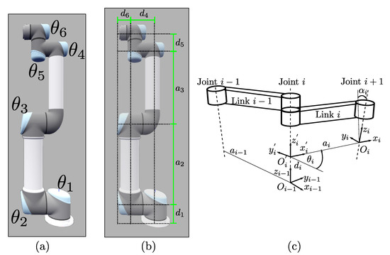
Figure 1.
(a) UR5 robot arm (figure generated using the library Robotics Toolbox for Python [35]). (b) DH parameters for robot link lengths (c) Standard DH graphical representation.
It comprises six rotational joints providing six degrees of freedom. To approximate the robot motors’ currents, the robot’s dynamic model and the torque-current relationship are proposed to estimate the currents synthetically.
The Denavit-Hartenberg (DH) parameters presented in Table 1 allow the description of the robot through four characteristics that enable the calculation of the positions of the different joints of the robot using transformation matrices obtaining the kinematic model, for which it is recommended to review the following source for the forward and inverse models [36].

Table 1.
Denavint-Hatenberg parameters for a UR5 manipulator.
- is the angle between the axes and around , taken as positive in a counter-clockwise rotation. The axis is located according to the right-hand rule.
- is the coordinate of along the axis .
- is the distance from to .
- is the angle between and around , taken positive in a counter-clockwise rotation.
On the other hand, the dynamic model of the robot allows for estimating the robot’s behavior considering the forces present in the system. Equation (1) describes the motion of the robot
and it is composed by the inertia matrix , Coriolis and centrifugal matrix , gravity vector , torque vector ,the articular position q, velocity , and acceleration vectors. To implement the model, it is necessary to know additional information about the physical properties of the joints and motors.
Table 2 shows each joint’s mass parameters, the center of mass coordinates, and the corresponding inertia tensor.
Table 2.
Dynamic parameters for the links of a UR5 robotic arm.
Table 3 shows the parameters corresponding to the motor inertia , gear ratio G, drive viscous friction B, and Coulomb friction .
Table 3.
Dynamic parameters for the motors of a UR5 robotic arm.
Note that the manufacturer provides all the parameters, except the drive viscous friction B, in different media and can be consulted in summary form in [37]. Parameter B has been proposed in a heuristic way since the calculation and modeling of the friction for the joints of the robot are outside the main objective of this work.
From the Equation (1) also can be expressed in terms of the relationship between torque and current (2):
where is the estimated torque of the model considering the effects of friction and without the intervention of external forces, and are the torque constants, and the motor current for the joint i, respectively. To estimate the motor current from the torque, a linear model proposed in [38] is used, where the torque constants and an offset are obtained, with which they establish a relationship between the modeled torque and the measured current. These parameters are proposed to compute the inverse process and estimate the motor current from a modeled torque. Equation (2) is reformatted as Equation (3):
where the term represents the offset of the linear model for the respective joint i. The values of the parameters for , and for .
The UR5 robot is commonly utilized in cooperative tasks and robotics research projects. Additionally, there are toolboxes available for different platform software which facilitates programming and controlling the robot. Moreover, there exists a publicly accessible dataset specifically based on this robot, which has been utilized for exploring and studying robot accuracy degradation.
2.2. Discrete Wavelet Transform
The discrete wavelet transform (DWT) is a mathematical method that gives time-frequency information of a signal [39]. The signal is separated into different frequency bands by passing through a filtering process. The process involves convolving the signal of interest with a transform function known as the mother wavelet, which determines the parameters of the high-pass and low-pass filters. In simpler terms, DWT allows a signal to be separated into its frequency components, which makes it possible to identify frequency changes over time. The complete process consists of two stages; first, the calculation of the approximation and detail coefficients is made, and second, the signal at the required level of decomposition is reconstructed using the coefficients of the previous stage in a process known as inverse DWT.
Equation (4) defines the DWT of a discrete-time signal with k samples, and represents the discrete mother wavelet used for decomposition level i
The selection of the wavelet mother family depends on the application; the most common families are Meyer, Haar, and Daubechies, among others. The Daubechies family is used in this work due to its characteristics of the higher number of vanishing moments [40], compact support in the frequency domain, and conserving the energy of the signal [41].
DWT algorithm consists of the following steps and is represented in Figure 2a,b:
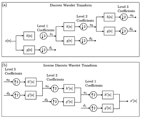
Figure 2.
Block diagram of (a) DWT decomposition process of a signal . (b) Inverse DWT reconstruction diagram of a signal .
- Define the wavelet mother function or wavelet basis and the decomposition level i to be used.
- The wavelet mother function provides the high-pass and low-pass filter coefficients.
- Perform the convolution operation between the signal and the filters to separate the signal into high and low-frequency bands.
- Downsample by two filtered signals obtained in the previous step, keeping the even-indexed samples.
- The outputs of filtering and downsampling the signal provide the detail vector and the approximation vector of the high-pass and low-pass filtering, respectively, at each decomposition level i.
- Repeat the filtering and downsampling process using the previous approximation output as input for the next decomposition level until all levels are completed.
- To reconstruct the approximation and detail branches of the signal for a specific level i, upsample the corresponding coefficient vectors and by a factor of 2 (adding zeros in the positions of the removed samples in the downsampling process, if necessary).
- Apply the corresponding time-inverse high-pass or low-pass filter coefficients.
- The signal reconstruction is obtained by the inverse process using the last approximation vector and all the detail vectors , .
DWT’s recent applications include condition monitoring of slew bearings [42], evaluation of plant growth status [43], and wind power prediction [44].
Robot operating conditions in industrial environments involve different factors such as disturbances, noise, temperature, humidity, and others. The acquisition of robot signals in a noisy environment requires the use of signal processing techniques to handle the noise. In this sense, it is necessary to perform an analysis of the signal of interest to determine, depending on its characteristics, which type of techniques to use, such as high-pass or low-pass filtering. On the other hand, time-frequency analysis techniques such as DWT allow the separation of the original signal into different parts that are already filtered while preserving the original characteristics of the signal. DWT is used in this work because it allows for the decomposition of a signal into different frequency bands using a series of filters, which is useful when dealing with noisy signals. Each frequency band can be independently analyzed, compressing the signal information and reducing the computational burden for further analysis. Additionally, the DWT algorithm and its inverse can be converted to matrix operations, facilitating its implementation in FPGA-based digital systems.
2.3. Statistical Indicators
Statistical indicators are used to find characteristics that help to know the behavior of a dynamic system. For this, they are applied to the signals of interest, and through these, it is possible to determine if there are changes or variations in the system at different moments in time. In this sense, the statistical indicators proposed in this work are the root mean square (RMS) value and the variance.
The RMS and variance metrics are useful for identifying patterns or anomalies within a signal. On one hand, RMS provides information about the signal’s amplitude or energy, while variance focuses on the signal’s dispersion around the average amplitude. Additionally, the calculation of both metrics is similar and can be easily implemented in an FPGA-based system. This allows for the optimization of the structure to perform the calculations of both metrics without the need for separate structures.
These indicators have been widely used in applications such as fault diagnosis in transformers [45] and bearings [46], among others.
The Root Mean Square (RMS) defined by Equation (5) value of a dataset or a discrete-time waveform is the square root of the arithmetic mean of the squares of the values
The variance measures the dispersion of a data set with respect to the mean and is defined by the Equation (6)
2.4. Artificial Neural Network
Artificial neural networks (ANN) emulate the computational processes performed by neurons in the human brain, using mathematical models. At the core of an ANN is the fundamental building block known as a simple perception and its structure is shown in Figure 3a.
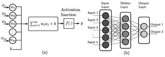
Figure 3.
(a) General diagram of a simple perceptron. (b) Simplified diagram of an artificial neural network, the connections between layers represent a multi-layer perception network.
A simple perceptron is a mathematical unit that represents a neuron. It takes in a vector input x of size m and performs a series of operations. First, the input vector is multiplied by a weight vector w, and the products are then summed together with a bias coefficient b. The resulting value is then passed through an activation function , such as binary step, linear, sigmoid, or hyperbolic tangent, to produce the output y. An Artificial Neural Network (ANN) consists of a collection of interconnected basic perceptions. The most common is the multi-layer perceptron (MLP), which is a network where all the neurons in the input, hidden, and output layers are interconnected. This configuration is shown in Figure 3b.
ANNs find utility in classification, learning, and pattern recognition tasks and are extensively employed across various scientific domains. For instance, some of their recent uses are the early diagnosis of breast cancer [47] and the combination with bio-inspired algorithms to improve the ANN training process [48].
Specifically, MLP possesses favorable attributes such as straightforward implementation, efficient training time, and the ability to generate high-quality models [49]. Additionally, the hardware implementation of MLP is relatively simple compared to other neural network architectures. Consequently, this work proposes the utilization of MLP based on these advantageous characteristics.
2.5. Proposed Methodology
The proposed methodology to determine if there is a deviation in the joints of a manipulator robot through the analysis of its motor currents is presented in a general way in Figure 4.
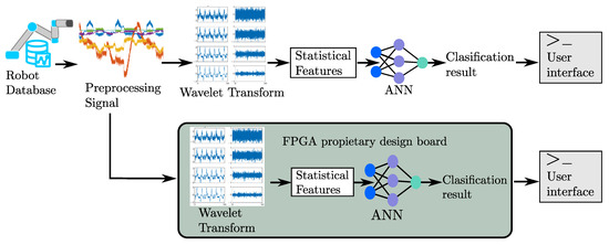
Figure 4.
General diagram of the proposed methodology.
In this work, it is considered that the calibration conditions of the robot, as well as its electromechanical components, are in optimal operating conditions. However, robot calibration is a procedure that is performed with external sensors or with the tools provided by the manufacturers. In this sense, the implementation of robot calibration algorithms in FPGA involves not only the implementation of these but also the development and implementation of control or communication systems to operate the robot along with all subsystems that this entails, this aspect is subject to the limitation of the logical resources of the FPGA device and the resolution of the processing of fixed point operations and it is beyond the scope of this work.
The proposed method starts with the database of the robot to be analyzed; for this, a synthetic and a real-world dataset are used. The current signals of the robot motors are required when performing a repetitive trajectory or task for a prolonged time. Signals are acquired at two different moments: at the beginning of the trajectory or task and hours after the task’s start. In this way, the dataset contains signals with different operating conditions, named cold operation (CO) for the initial state and hot operation (HO) for the second state. Figure 5a–f shows the real-world dataset motor current signals of joints one to six during the CO state.

Figure 5.
Real-world dataset current joints signal. Plots (a–f) show the signal for joints one to six.
In the pre-processing of the signals to provide robustness to the method, different noise levels are added to the signals in the dataset. These noisy signals are then employed in subsequent process stages as a dataset. The noise levels used are 5 dB, 10 dB, 15 dB, and 20 dB. Figure 6a,b show the current signal for CO and HO states from the real-world dataset, respectively, both with 5 dB of noise.

Figure 6.
Real-world dataset joint one signal with 5 dB of noise. (a) CO state signal. (b) HO state signal.
Subsequently, the signals are divided into windows of 256 samples. In this point according to Figure 4, there are two branches; the first branch involves the implementation of the proposed method through software simulation, and its description is provided below. The second branch focuses on the hardware implementation of the method using an FPGA-based system, and this aspect is covered in the subsequent section. Since the DWT maintains the characteristics of the original signal through the different frequency bands, the windowed signals are processed with the DWT to find differences associated with the joint deviation of the robot. The wavelet mother Daubechies order six is used to perform the analysis. However, as shown in [18], only the first four levels are considered relevant for the analysis due to the amplitude and narrow frequency bands of the last two decomposition levels. Additionally, due to the FPGA system memory resources, and the DWT soft-core functionality, only levels three and four are used for the analysis. Figure 7 presents the DWT decomposition at level four for the joint one, with 5 dB noise added from the real-world dataset. Figure 7a,b represent the approximation and details of the CO state, respectively. On the other hand, Figure 7c,d display the results for the HO state.
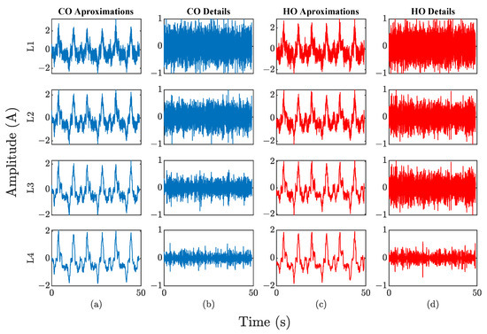
Figure 7.
Real-world dataset joint one with 5 dB of noise DWT decomposition level 4. (a) CO state signal approximation components. (b) CO state signal details components. (c) HO state signal approximation components. (d) HO state signal details components.
Afterward, for the approximations and details of levels 3 and 4 of each signal, the RMS and variance indices are calculated; this process is repeated with each window that makes up the original signal. Subsequently, the indicators corresponding to each signal are averaged over the number of windows. This process is applied to each signal in the dataset, and the obtained indices are used for training, validation, and testing of a classifier based on ANN. To perform the complete robot analysis, the above process is replicated for each robot joint exploiting the FPGA’s concurrent processing capability. In this case, for a UR5 robot, there are six classifiers based on ANN. In this way, each classifier keeps a simple configuration and the resource consumption for the hardware implementation of the whole process is kept below the capacity of the proprietary FPGA board.
Finally, the soft-cores for DWT, statistical features calculation, and neural network classifier are developed to validate the method implementation in an FPGA system, and the classifier results are displayed to the user in a command line terminal. The proposed methodology is tested in two synthetic and one real scenario for this work. For the synthetic scenario, the robot’s database is obtained through the dynamic modeling of the robot and its simulation, performing a parametric trajectory as shown in Figure 8a.
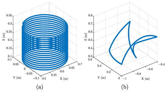
Figure 8.
Trajectories followed by the robot. (a) Synthetic case. (b) Real case.
The trajectory parameters presented in Equation (7) are the radius of the helix m, the final height m, the frequency of the helix , and time s.
The sampling frequency of the UR5 robot is 125 Hz; therefore, with the above parameters, the synthetic signals of the simulated robot have a total of 1024 samples. In the synthetic scenario, one data set consists of the trajectory signals without deviation, which is the initial CO state. Six different data sets are generated for the HO state, and the deviation at each of the different joints of the robot is added. A sinusoidal signal is added to the robot’s joint position signal obtained by following the helix trajectory to simulate the deviation. The sinusoidal signal has a randomly generated amplitude of 1 to 10% of the maximum amplitude value of the robot’s joint position signal, a frequency of , and a time of s. This way, six HO datasets with 50 synthetic signals are obtained; each set contains random deviation levels in different joints. Each signal in the dataset generates ten additional signals for each noise level by adding white Gaussian noise (5 dB, 10 dB, 15 dB, and 20 dB), resulting in 2000 signals for each HO state dataset. For the CO dataset, one signal without deviation is processed similarly to obtain 500 signals per noise level. Combining the HO and CO datasets gives 4000 signals for the cases with joint deviation.
On the other hand, for the real case, a public-access dataset provided by the National Institute of Standards and Technology (NIST) is used [50]. Different speed levels test for the robot are provided in the dataset (50% and 100% speed). In this work, the dataset corresponding to the 100% speed of the robot is used. Like the synthetic case, the robot used is the UR5. The signals from the robot actuators were received at the controller level. The frequency was 125 Hz.
Figure 8b presents the trajectory used in this dataset. The robot continuously follows the trajectory with a weight of 4.5 lb on its end-effector for approximately 2 h. The CO status signals are captured when the robot has just started, and the HO status signals are obtained after 2 h of continuous operation. Three signals are provided for each robot’s operation state: CO and HO, and the size of the signals was adjusted to obtain exact powers of 2 and to divide each signal into three parts of 2048 samples for a set of nine signals for each CO and HO state.
As was done with the synthetic dataset and to augment the dataset size, 50 new signals are generated from each of the nine original signals by applying white Gaussian noise at each noise level. This results in 3600 signals, with 1800 for each HO and CO data set. For each signal in the data set, the approximation and details of levels three and four are used to calculate the variance and RMS features, which means that each signal has eight features that are used as input to the neural network. So the datasets have a size of 4000 × 8 and 3600 × 8. For the neural network classifier, the datasets are split as follows: 70% for training, 15% for validation, and 15% for testing. The neural network comprises one input layer of size eight, a hidden layer of 16 neurons, and an output layer of size two. Besides, it is trained for 1000 epochs, using the Adam optimizer and the mean square error loss function. The activation function for the hidden and output layers is sigmoid.
With the dataset of the synthetic and real scenarios prepared, we proceed to describe the hardware implementation of the proposed method.
2.6. Positional Accuracy Degradation FPGA Implementation
Figure 9 shows a block diagram of the hardware implementation of the proposed methodology to determine if there is a deviation in the joints of the robot through the analysis of motor currents.

Figure 9.
General scheme of the FPGA implementation of the proposed method.
Starting from the fact that there is a dataset of current signals from the robot’s motors, as previously mentioned, the signal to be processed is divided into windows; these windowed signals are stored in the RAM of the processing card. The signal information corresponding to its first window is loaded into the FPGA. Then DWT coefficients corresponding to the first stage are loaded, and the DWT process is performed in the FPGA for that particular stage. Subsequently, information on the frequency band obtained in this process is moved to the calculation process of the RMS and variance statistical indicators. The indicators obtained are saved in the device’s RAM at the end of the calculation. Later, the previously described procedure is repeated until the four stages, which correspond to the approximation and detail of decomposition levels three and four, are completed.
When the calculation and storage of the statistical indicators of the approximations and details of levels three and four have been completed, they are moved to the FPGA processing of the classifier based on neural networks, where the classification obtained with the network is stored in the memory of the device. Subsequently, the window signal for the next joint is loaded, and the entire process is repeated until all six articulations have been completed.
Figure 10 shows the general configuration of the system used to carry out the hardware implementation.
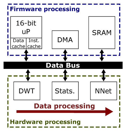
Figure 10.
General diagram of the FPGA system.
The system comprises firmware processing containing 16-bit microprocessor modules, direct memory access (DMA), and Static Random Access Memory (SRAM). Whereas the hardware processing part comprises the DWT, statistical, and neural network models connected to the firmware processing through the data bus. Below are the modules corresponding to the main processes implemented in the FPGA, such as the DWT, the calculation of statistical indicators, and the neural network.
The proposed methodology was implemented in a digital system using a low-cost proprietary designed board that is based on an FPGA. This framework is specifically designed for in-situ online data processing, eliminating the need for external communication with other systems for data processing. The board is equipped with a low-cost Spartan 6 XC6SLX45 FPGA with a clock frequency of 48 MHz; it also features static random-access memory (RAM), communication ports such as the universal serial bus (USB), and universal asynchronous receiver transmitter (UART), power management, and flash memory. A 16-bit xQuP01v0 processor is embedded in the FPGA, besides an interconnection in-system bus (ISB), both proprietary designs; a broader description of the applications of the FPGA-based proprietary board can be found in [51,52]. The input data used in the system is scaled to an input range of , and signal data are converted to a binary stream in fixed-point format saved in onboard flash memory. As the process is executed, the microprocessor embedded in the FPGA uploads the data from the flash to the hardware calculation units and, when finished, reports the result via a USB to a user interface.
2.6.1. DWT Soft-Core FPGA Module
The DWT soft-core module calculates the decomposition of a signal in different approximation and detail frequency bands and performs the original signal reconstruction. This process is realized through a matrices multiplications. Figure 11 shows the module’s architecture for the DWT process.
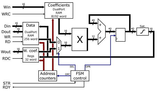
Figure 11.
Architecture diagram of the DWT soft-core.
Within this module, the data corresponding to the windowed signal of 256 samples and the coefficient module are read from RAM. The coefficients module contains the wavelet matrices with wavelet filter values for approximations and details of levels three and four of the mother wavelet Daubechies order six. The “W. coef.” module stores the wavelet coefficient vectors obtained by multiplying the wavelet matrix with the input signal. For reconstruction, the stored data in “W. coef.” is read and multiplied by the transposed wavelet matrix corresponding to the respective level, approximation, or detail. These matrices are stored in “coefficients” in RAM. The result of the decomposition and reconstruction of the frequency bands is saturated at 16 bits and is stored in the “Data” and “W. coef.” modules. Figure 11 depicts the bit size changes after each operation. A finite state machine (FSM) controls the signal decomposition and reconstruction process selection. It is done through the SEL signal and memory addresses of the coefficients, data, and wavelet coefficients modules. The address counters contain this information, and the FSM chooses the active module using the OPC signal. The STR signal indicates to FSM the beginning of the process, and once it is completed, the RDY signal is activated. To write and read memory, the modules use the WRC, WR, RD, and RDC signals. DWT module performs the process for the approximations and details of levels three and four of the signal stored in “Data”. Once the process is finished, the reconstructed frequency bands are transferred to the statistical module for further processing.
2.6.2. Statistics Soft-Core FPGA Module
The Statistics soft-core module calculates a discrete input signal’s RMS and variance features. The module comprises a single structure, and different indicators can be calculated by changing the data path. Figure 12a shows the general diagram of the architecture of the statistics module. It comprises three blocks: a first-input first-output memory storage block, the Datapath block where the index calculation is carried out, and an FSM block that conducts the operation of the process.
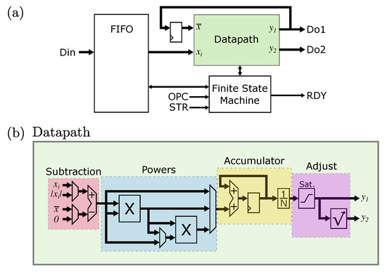
Figure 12.
Architecture Statistics soft-core. (a) General core diagram. (b) Datapath module.
In the initial process, when the STR signal is activated in the FSM, the choice of the statistical indicator to be calculated is made with the OPC signal. At the end of the calculation, the RDY flag is activated. The input data to the module (Din) is stored in memory in the FIFO block to enter the Datapath block later, and the Do1 and Do2 outputs obtain the calculation of the index.
The process carried out within the datapath block is shown in a general way in Figure 12b; it consists of four sections: subtraction, powers, accumulation, and adjustment. A subtraction is performed between the sample , or the absolute value of the sample , and the mean of the input signal . Subsequently, in the powers section, the result obtained in the subtraction is raised to different powers, as the case may be, from the first to the fourth power. The accumulated value of the previous operation is stored in the accumulator and divided by the number of samples N. Finally, the result is saturated to adjust the required bit size and is output by ; if it is necessary to apply the square root, the output is made by .
Figure 13a shows the module Datapath configured to calculate the variance for an input signal x; the connection is highlighted in red, and the operation’s progress is observed in the different sections of the module.
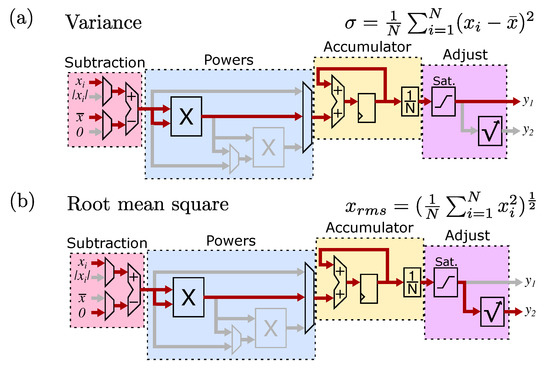
Figure 13.
Statistical features modules. (a) Variance module operation path. (b) RMS module operation path.
First, the difference between the sample and the mean of the signal is calculated; second, it is squared in the powers section, the accumulation is divided by the number of samples, and after saturation, the indicator completed by the output is obtained. To calculate the RMS index, the process is presented in Figure 13b, wherein the subtraction section of the IPcore of the sample is subtracted with a zero, which does not modify the value of the sample, then it is squared. In the powers section, the accumulated value is divided by the number of samples; at saturation output, the square root is calculated, and the result is delivered by . When the indicators of the approximation and detail frequency bands of levels three and four have been calculated (eight indicators), they are moved to the neural network-based classifier module.
2.6.3. Neural Network Soft-Core FPGA Module
The neural network soft-core module performs the process of a trained network for classification; a description of its components is provided below. Figure 14a shows the general diagram of a simple perceptron.

Figure 14.
(a) Architecture diagram of a simple perceptron. (b) Diagram of neural layer core. (c) Neural network layer architecture diagram.
It is composed of a multiplier where input is multiplied by the weights , where i represents the input number, and j is the weight number. A register accumulates the result, and the bias is added. Afterward, the operation result is saturated to maintain the required bit size, and the activation function, contained in a look-up table (LUT), is continued. Finally, the output is delivered via .
Figure 14b shows a general diagram of a set of perceptrons composing a neural network layer. This module comprises different blocks: a block of weights, a block of counters, FMS, bias, and an activation function. The block of weights contains the weights corresponding to neuron M and N number of neurons in the layer. Furthermore, the counters block counts the number of neurons and their corresponding weights. The bias block contains the biases for M neurons. Additionally, the activation function block performs the procedure described above in the perceptron, and the FMS directs the entire layer process. Signal STR indicates the start of the calculation, RD and WR are signals for reading and writing data in memory, and the RDY signal indicates that the calculation is complete. Figure 14c presents the general diagram of the classifier based on neural networks. In this network configuration, an input layer stores the data that the network will evaluate in the FIFO 0 register through the Din input and the WR signal to control write enable in memory. The process starts when the STR signal is high, and the samples enter the structure presented in Figure 14b through the RD signal. Moreover, the hidden layer’s output is stored in FIFO 1 register by the signal WR. Once all the samples are complete, the RDY signal goes high and activates the next layer. The output layer of the network receives the data stored in FIFO 1 and performs the same process as mentioned in the hidden layer. The layer’s output is stored in the FIFO 2 register as the input data is processed. These are accessible when the output layer RDY signal is high and are readable by Dout and the RD control signal. Weights and biases of the hidden and output layers and the activation functions are stored in the device’s RAM. Neural network configuration consists of an input layer with eight inputs, a hidden layer of 16 neurons, and an output layer with two outputs; the activation functions are sigmoid. Neural network training was carried out in software independently, and the values of weights and bias were stored for use in the FPGA device.
3. Results and Discussion
The results of the proposed methodology to determine joint deviation in the robot using motor current analysis are presented below. The results are shown in the form of confusion matrices, and a summary in tabular form is provided to help interpret the findings. The confusion matrix chart has the correctly classified observations on its diagonal, while the cells outside the diagonal show the incorrect observations. In both cases, the percentage is shown. The last cell on the diagonal shows the average accuracy. Moving to the last column, the first two cells specifically present the percentages of all samples that were correctly and incorrectly classified for each class. These values correspond to precision and false discovery rate, respectively. Lastly, focusing on the last row, the two cells highlight the percentage of samples belonging to each class that were correctly and incorrectly classified. These values are commonly referred to as recall and false negative rate, respectively. In summary, the last cell of the confusion matrix diagonal shows the average number of samples that the ANN correctly and incorrectly classified, providing an overall accuracy measure for the classifier, this information for the real and synthetic cases is presented in Table 4.
Table 4.
Average accuracy obtained in the ANN validation process for the synthetic and real cases.
To evaluate the operation of the proposed method, a computer software simulation of the different techniques that make up the methodology was carried out. Additionally, to evaluate the classifiers 600 samples from each dataset were used for each corresponding joint; these samples account for 15% of the dataset for each of the six scenarios in the synthetic case. These samples were then separated from the original dataset and are treated as unknown samples for the ANN classifiers.
Figure 15 shows the confusion matrices obtained from the classifiers based on neural networks for the synthetic scenario and a summarized version is presented in Table 4.
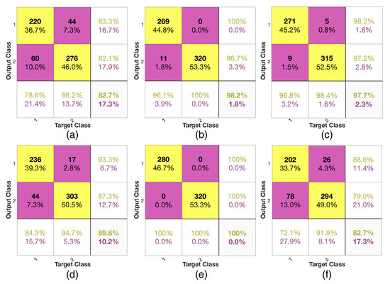
Figure 15.
Confusion matrices obtained in the ANN validation process for the synthetic cases where the deviation is induced in one of the robot joints at a time. (a–c) confusion matrices correspond to joints one to three. (d–f) confusion matrices correspond to joints four to six.
Figure 15a–c corresponds to the cases of joints one to three, while Figure 15d–f corresponds to joints four to six. In this sense, it is observed that the classifiers can differentiate between the states of operation when there is a deviation in the joints with a minimum average accuracy of 82.7% corresponding to joints one and six, while joint four has an average value of 89.8%, joints two and three have an average accuracy of around 97% and joint five has an average accuracy of 100%. It should be noted that for the synthetic scenario, each case includes a deviation in the respective joint. For instance, in case one, only joint one contains a deviation, while the other five joints remain unaffected. In this regard, joints two and three are well differentiated by their respective classifiers; this can be attributed to the fact that in the trajectory carried out, these joints have a more significant intervention than the rest.
In addition, in the motion equations of the robot, these joints are closely related; therefore, since this test is synthetic, the deviation of one joint can affect the behavior of the other. Regarding joint five, which presents 100% accuracy, this is attributable to its minimal intervention in the trajectory; therefore, by inducing deviation in the joint, the change between both operating states is differentiable by the proposed methodology. For joints, one, four, and six, the difference between their accuracy levels and those of the joints with the best ranking result can be inflated by their level of intervention in the trajectory and the fact that the synthetically induced deviation has a random amplitude.
On the other hand, for the real case, 540 samples were used to test the classifier. As in the synthetic case, these samples also represent 15% of the respective datasets used for training the classifiers and the samples are unknown to the classifiers. The confusion matrices obtained are presented in Figure 16, where Figure 16a–c correspond to articulations one to three and Figure 16d–f correspond to joints four through six and a summarized version is presented in Table 4.
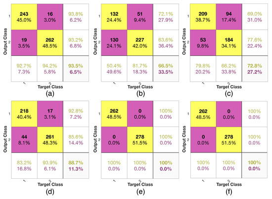
Figure 16.
Confusion matrices obtained in the ANN validation process for the real case where the deviation at joint five is known. (a–c) confusion matrices correspond to joints one to three. (d–f) confusion matrices correspond to joints four to six.
Figure 16 shows that for joints two and three, an average accuracy of 66.5% and 72.8% is obtained, respectively. Whereas for joints one and four, an average accuracy greater than 88% is obtained.
Furthermore, joints five and six present an average accuracy of 100%. These results are obtained from a real-world dataset; however, the dataset does not provide information on the condition of the robot at the time of obtaining the signals, so it is not possible to determine if there is a mechanical, electrical, or wear failure that has caused a joint failure deviation in the robot. In this sense, the results obtained for joints two and three indicate that the signals of the robot CO and HO’s operating states are not different. Additionally, the other joints have results greater than 90% accuracy, for which the classifier can distinguish the two states of operation and indicate a deviation. Emphasize that this dataset has a time difference of 2 h between the initial and final operating states, in addition to the fact that this robot performs a trajectory continuously with a mass of 4.5 lb and operates at 100% of its maximum speed, for which these results could be attributed to the additional inertia caused by the extra weight and speed of operation. The results obtained in the synthetic case and in the real case show that the proposed method can process signals with different noise levels using the DWT, using the DWT, which allows the noisy signal to be decomposed into different frequency bands without losing the characteristics of the original signal, thus enabling the utilization of the frequency band of interest.
Regarding the results of the implementation in the physical system, validation is made that the calculations made in the FPGA device correspond to those obtained in the software simulation. In this sense, Table 5 shows the performance obtained in the main modules used to implement the methodology on hardware. The information in the Table 5 consists of the clock cycles necessary to calculate the module and complete processing of the module (calculation and copy of data to the buffers), as well as the calculation time and complete processing of each module. It is observed that the module that requires less time to perform complete processing is the neural network, while the DWT is the module with the most extended duration. The DWT module decomposes and reconstructs the window of the signal to be analyzed; the module’s error for calculating the approximation levels is 0.006%, while for the details, it is 0.02%. The complete system implemented in FPGA includes the DWT, statistical, and neural network modules, the embedded microprocessor, internal data bus, and device drivers such as flash memory, USB, RAM, bootloader, debugger, and programmer, among others.
Table 5.
Module performance in hardware implementation.
Table 6 presents the resources of the FPGA device used for the implementation; it should be noted that this is a low-cost device and that, with the resources used, it is capable of calculating the entire process in less than a second. The resources are referred to in the “logic utilization” column. Specifically, the columns “Used”, “Available”, and “Utilization” indicate the total number of elements implemented, available elements, and the percentage of elements used, respectively. In general, according to the information in Table 6, it is possible to say that the device used half of its resources for this implementation.
Table 6.
System resource utilization.
The hardware-software execution time for the complete system is 564,720 ms. Before the neural network classifier, the average error between the software (e.g., Matlab) and the FPGA calculation for the modules before the classifier amounts to 0.87%. However, the accuracy obtained by the neural network module reaches 83% compared to the accuracy obtained in the software implementation. It should be noted that the accuracy obtained by the neural network and the average error are attributable to the fixed point representation. The results obtained from the hardware implementation validate the use of the proposed method to detect deviations in the robot’s joints through the analysis of the motor currents.
Regarding the results obtained in this work, it should be noted that specifically for joint five of the real case, the results coincide with those reported in [53], where the same dataset was used, and a manual analysis of velocity and position graphs of the joint was conducted without a systematic approach. In another study [17] MRA and DLSTM are used to obtain the residual error of the end-effector of the robot. However, it is not determined in which joint exhibited deviation causing the error in the end-effector. On the other hand in [18] an expert system based on two neural networks, dimension reduction, and energy and fractal indicators was presented. This system aimed to accurately detect deviations in the robot’s joints. However, implementing the fractal approach in FPGA was found to be more complex than the statistical indicators proposed in this current study. It’s worth noting that the aforementioned studies were performed using software simulation and offline analysis, which didn’t pose resource limitations or fixed-point operation issues, in contrast with an FPGA system. The method proposed identifies in which joint of the robot there is deviation, uses techniques and algorithms that are easy to implement on FPGA systems, and employs a low-cost self-designed board that operates independently without the need for external systems which allows for systematic in-situ analysis.
4. Conclusions
The importance of robotic systems in modern manufacturing processes requires high accuracy and precision to perform tasks with high-quality standards, such as painting, welding, and machining. Achieving this level of precision is critical for the robot’s performance, but various factors can degrade it, such as wear and failure of mechanical and electrical components or environmental conditions. In this sense, a methodology for the detection of joint deviation of the robot through the current analysis of the actuators and its implementation in a digital system based on an FPGA is introduced in this work. Synthetic signals, both with and without deviation, are generated using the dynamic model of a UR5 robot. Real-world data from a UR5 robot validates the methodology. To enhance the method’s robustness, the signals are contaminated with different noise levels. Then the signals are processed using DWT to separate them into approximation and detail frequency bands, and statistical indicators such as RMS and variance are calculated for each band. Finally, the indicators are used to train and validate a classifier based on neural networks. From the results is concluded that:
- The proposed method is able to work with signals containing noise due to the use of the DWT to decompose the signal into different frequency bands, which allows an analysis of the signals with a smaller amount of information than the original signal. Its implementation in hardware allows the decomposition and reconstruction of the signal with a single module, which allows better management of FPGA resources.
- The statistical indicators used have proven to be effective in the detection of non-visible features in the analyzed signals, they are simple and their hardware implementation has been carried out through a module with a versatile architecture that allows the calculation of other statistical indicators if necessary.
- The classifier, based on an MLP network, showed its effectiveness in differentiating between the different operating states of the signals provided by the statistical indicators. In this sense, the classifier structure is simple with a reduced number of neurons in the hidden layer, which makes its implementation in hardware not complex.
- For the particular case of joint five of the real case, the result is in line with the findings reported in [53], which also highlights the deviation in that joint.
- The designed modules and architectures have been implemented in a low-cost proprietary FPGA-based digital system and have demonstrated the feasibility of the proposed method using about 50% of the resources. In addition to achieving a high processing speed for all joints (less than one second) with minimal error attributed to truncation and fixed point operations. Moreover, the use of an FPGA system allows for concurrent execution and reconfiguration of the device; if an additional module is required, it can be incorporated into the system.
Future work proposes the hardware implementation of a method capable of performing the analysis of the positional degradation of the robot using only a classifier based on neural networks, as well as analyzing the classifier’s behavior when multiple joints deviate simultaneously. Furthermore, the proposal includes the exploration of other non-linear indicators, signal processing techniques, and methodologies based on machine learning and deep learning.
Author Contributions
Conceptualization, E.G.-U., R.A.O.-R. and L.M.-V.; methodology, E.G.-U., R.A.O.-R. and L.M.-V.; software, validation, and formal analysis, E.G.-U. and L.M.-V.; investigation, E.G.-U., R.A.O.-R. and L.M.-V.; resources, E.G.-U., R.A.O.-R. and L.M.-V.; writing—original draft preparation, E.G.-U., R.A.O.-R. and L.M.-V.; writing—review and editing, E.G.-U., R.A.O.-R. and L.M.-V.; visualization, E.G.-U. and R.A.O.-R.; supervision, R.A.O.-R. and L.M.-V.; project administration, R.A.O.-R. and L.M.-V.; funding acquisition, R.A.O.-R. and L.M.-V. All authors have read and agreed to the published version of the manuscript.
Funding
This work was supported by the Consejo Nacional de Ciencia y Tecnología (CONACYT) under scholarship 783320 and grant FONDEC-UAQ-2021-LMV-6829.
Institutional Review Board Statement
Not applicable.
Informed Consent Statement
Not applicable.
Data Availability Statement
Not applicable.
Conflicts of Interest
The authors declare no conflict of interest.
Abbreviations
The following abbreviations are used in this manuscript:
| ANN | Artificial Neural Network |
| BUFG | Global Buffer |
| BUFGCTRLs | Global Clock Control Buffer |
| CO | Cold Operation |
| Din | Data input |
| DMA | Direct Memory Access |
| Do1 | Data output 1 |
| Do2 | Data output 2 |
| Dout | Data output |
| DSP48A1s | Digital Signal Processing element included on certain FPGAs |
| DWT | Discrete Wavelet Transform |
| FIFO | First-input First-output |
| FPGA | Field Programmable Gate Array |
| FSM | Finite State Machine |
| HO | Hot Operation |
| IOBs | Input Output Blocks |
| IPcore | Intellectual Propriety Core |
| ISB | In-System Bus |
| LUT | Look-Up Table |
| LUT-FF | Look-Up Table-Flip-Flop |
| MLP | Multi-layer Perceptron |
| OPC | Option Control signal |
| OPR | Option Register signal |
| RAM | Random Access Memory |
| RD | Read signal |
| RDC | Read Coefficient signal |
| RDY | Ready signal |
| RMS | Root Mean Squared |
| SEL | Select signal |
| SRAM | Static Random Access Memory |
| STR | Start signal |
| UART | Universal Asynchronous Receiver-Transmitter |
| Win | Window input |
| Wout | Window output |
| WR | Write signal |
| WRC | Write Coefficient signal |
References
- Kelaiaia, R.; Chemori, A.; Brahmia, A.; Kerboua, A.; Zaatri, A.; Company, O. Optimal dimensional design of parallel manipulators with an illustrative case study: A review. Mech. Mach. Theory 2023, 188, 105390. [Google Scholar] [CrossRef]
- Brahmia, A.; Kelaiaia, R.; Company, O.; Chemori, A. Kinematic sensitivity analysis of manipulators using a novel dimensionless index. Robot. Auton. Syst. 2022, 150, 104021. [Google Scholar] [CrossRef]
- Qiao, G.; Weiss, B.A. Industrial Robot Accuracy Degradation Monitoring and Quick Health Assessment. J. Manuf. Sci. Eng. 2019, 141, 071006. [Google Scholar] [CrossRef]
- Zhang, Y.; An, H.; Ding, X.; Liang, W.; Yuan, M.; Ji, C.; Tan, J. Industrial Robot Rotate Vector Reducer Fault Detection Based on Hidden Markov Models. In Proceedings of the 2019 IEEE International Conference on Robotics and Biomimetics (ROBIO), Dali, China, 6–8 December 2019; pp. 3013–3018. [Google Scholar] [CrossRef]
- Wescoat, E.; Kerner, S.; Mears, L. A comparative study of different algorithms using contrived failure data to detect robot anomalies. Procedia Comput. Sci. 2022, 200, 669–678. [Google Scholar] [CrossRef]
- Truc, L.N.; Quang, N.P.; Quang, N.H. Impact analysis of actuator torque degradation on the IRB 120 robot performance using simscape-based model. Int. J. Electr. Comput. Eng. (IJECE) 2021, 11, 4850. [Google Scholar] [CrossRef]
- Rohan, A. Deep Scattering Spectrum Germaneness for Fault Detection and Diagnosis for Component-Level Prognostics and Health Management (PHM). Sensors 2022, 22, 9064. [Google Scholar] [CrossRef]
- Raviola, A.; Martin, A.D.; Guida, R.; Jacazio, G.; Mauro, S.; Sorli, M. Harmonic Drive Gear Failures in Industrial Robots Applications: An Overview. In Proceedings of the PHM Society European Conference, Virtual Event, 28 June–2 July 2021; Volume 6. [Google Scholar]
- Lo, C.C.; Lee, C.H.; Huang, W.C. Prognosis of Bearing and Gear Wears Using Convolutional Neural Network with Hybrid Loss Function. Sensors 2020, 20, 3539. [Google Scholar] [CrossRef]
- Lu, K.; Chen, C.; Wang, T.; Cheng, L.; Qin, J. Fault diagnosis of industrial robot based on dual-module attention convolutional neural network. Auton. Intell. Syst. 2022, 2, 12. [Google Scholar] [CrossRef]
- Rohan, A.; Raouf, I.; Kim, H.S. Rotate Vector (RV) Reducer Fault Detection and Diagnosis System: Towards Component Level Prognostics and Health Management (PHM). Sensors 2020, 20, 6845. [Google Scholar] [CrossRef]
- Long, J.; Mou, J.; Zhang, L.; Zhang, S.; Li, C. Attitude data-based deep hybrid learning architecture for intelligent fault diagnosis of multi-joint industrial robots. J. Manuf. Syst. 2021, 61, 736–745. [Google Scholar] [CrossRef]
- Zhou, X.; Zhou, H.; He, Y.; Huang, S.; Zhu, Z.; Chen, J. Harmonic reducer in-situ fault diagnosis for industrial robots based on deep learning. Sci. China Technol. Sci. 2022, 65, 2116–2126. [Google Scholar] [CrossRef]
- Pan, J.; Qu, L.; Peng, K. Sensor and actuator fault diagnosis for robot joint based on deep CNN. Entropy 2021, 23, 751. [Google Scholar] [CrossRef] [PubMed]
- Pan, J.; Qu, L.; Peng, K. Deep residual neural-network-based robot joint fault diagnosis method. Sci. Rep. 2022, 12, 17158. [Google Scholar] [CrossRef]
- Jiao, J.; Zheng, X.J. Fault diagnosis method for industrial robots based on DBN joint information fusion technology. Comput. Intell. Neurosci. 2022, 2022. [Google Scholar] [CrossRef] [PubMed]
- Taha, H.A.; Yacout, S.; Birglen, L. Detection and monitoring for anomalies and degradation of a robotic arm using machine learning. In Advances in Automotive Production Technology–Theory and Application; Springer: Berlin/Heidelberg, Germany, 2021; pp. 230–237. [Google Scholar] [CrossRef]
- Galan-Uribe, E.; Amezquita-Sanchez, J.P.; Morales-Velazquez, L. Supervised Machine-Learning Methodology for Industrial Robot Positional Health Using Artificial Neural Networks, Discrete Wavelet Transform, and Nonlinear Indicators. Sensors 2023, 23, 3213. [Google Scholar] [CrossRef]
- Qiao, G.; Weiss, B.A. Quick health assessment for industrial robot health degradation and the supporting advanced sensing development. J. Manuf. Syst. 2018, 48, 51–59. [Google Scholar] [CrossRef]
- Qiao, G.; Garner, J. Advanced Sensing Development to Support Accuracy Assessment for Industrial Robot Systems. In Proceedings of the ASME 2020 15th International Manufacturing Science and Engineering Conference, Virtual Online, 3 September 2020. [Google Scholar] [CrossRef]
- Qiao, G. Advanced Sensing Development to Support Robot Accuracy Assessment and Improvement. In Proceedings of the 2021 IEEE International Conference on Robotics and Automation (ICRA), Xi’an, China, 30 May–5 June 2021; pp. 917–922. [Google Scholar] [CrossRef]
- Izagirre, U.; Andonegui, I.; Eciolaza, L.; Zurutuza, U. Towards manufacturing robotics accuracy degradation assessment: A vision-based data-driven implementation. Robot. Comput.-Integr. Manuf. 2021, 67, 102029. [Google Scholar] [CrossRef]
- Liu, Y.; Li, Y.; Zhuang, Z.; Song, T. Improvement of Robot Accuracy with an Optical Tracking System. Sensors 2020, 20, 6341. [Google Scholar] [CrossRef]
- Sun, Z.; Xu, Y.; Ma, Z.; Xu, J.; Zhang, T.; Xu, M.; Mei, X. Field Programmable Gate Array Based Torque Predictive Control for Permanent Magnet Servo Motors. Micromachines 2022, 13, 1055. [Google Scholar] [CrossRef]
- Liu, W.; Zhao, C.; Liu, Y.; Wang, H.; Zhao, W.; Zhang, H. Sim2real kinematics modeling of industrial robots based on FPGA-acceleration. Robot. Comput.-Integr. Manuf. 2022, 77, 102350. [Google Scholar] [CrossRef]
- Cabrera-Rufino, M.A.; Ramos-Arreguín, J.M.; Rodríguez-Reséndiz, J.; Gorrostieta-Hurtado, E.; Aceves-Fernandez, M.A. Implementation of ANN-Based Auto-Adjustable for a Pneumatic Servo System Embedded on FPGA. Micromachines 2022, 13, 890. [Google Scholar] [CrossRef]
- Liu, C.C.; Lee, T.T.; Xiao, S.R.; Lin, Y.C.; Lin, Y.Y.; Wong, C.C. Real-time FPGA-based balance control method for a humanoid robot pushed by external forces. Appl. Sci. 2020, 10, 2699. [Google Scholar] [CrossRef]
- Zhang, C.; Chen, S.; Zhao, L.; Li, X.; Ma, X. FPGA-Based Linear Detection Algorithm of an Underground Inspection Robot. Algorithms 2021, 14, 284. [Google Scholar] [CrossRef]
- Romanov, A.M.; Romanov, M.P.; Manko, S.V.; Volkova, M.A.; Chiu, W.Y.; Ma, H.P.; Chiu, K.Y. Modular reconfigurable robot distributed computing system for tracking multiple objects. IEEE Syst. J. 2020, 15, 802–813. [Google Scholar] [CrossRef]
- Plancher, B.; Neuman, S.M.; Bourgeat, T.; Kuindersma, S.; Devadas, S.; Reddi, V.J. Accelerating robot dynamics gradients on a cpu, gpu, and fpga. IEEE Robot. Autom. Lett. 2021, 6, 2335–2342. [Google Scholar] [CrossRef]
- Żabiński, T.; Hajduk, Z.; Kluska, J.; Gniewek, L. FPGA-Embedded Anomaly Detection System for Milling Process. IEEE Access 2021, 9, 124059–124069. [Google Scholar] [CrossRef]
- Huang, C.H.; Chen, P.J.; Lin, Y.J.; Chen, B.W.; Zheng, J.X. A robot-based intelligent management design for agricultural cyber-physical systems. Comput. Electron. Agric. 2021, 181, 105967. [Google Scholar] [CrossRef]
- Cañas, J.M.; Fernández-Conde, J.; Vega, J.; Ordóñez, J. Reconfigurable computing for reactive robotics using open-source fpgas. Electronics 2021, 11, 8. [Google Scholar] [CrossRef]
- Pan, J.; Luan, F.; Gao, Y.; Wei, Y. FPGA-based implementation of stochastic configuration network for robotic grasping recognition. IEEE Access 2020, 8, 139966–139973. [Google Scholar] [CrossRef]
- Corke, P.; Haviland, J. Not your grandmother’s toolbox–the Robotics Toolbox reinvented for Python. In Proceedings of the 2021 IEEE International Conference on Robotics and Automation (ICRA), Xi’an, China, 30 May–5 June 2021; pp. 11357–11363. [Google Scholar]
- Kebria, P.M.; Al-Wais, S.; Abdi, H.; Nahavandi, S. Kinematic and dynamic modelling of UR5 manipulator. In Proceedings of the 2016 IEEE International Conference on Systems, Man, and Cybernetics (SMC), Budapest, Hungary, 9–12 October 2016; pp. 004229–004234. [Google Scholar]
- Porcelli, G. Dynamic Parameters Identification of a UR5 Robot Manipulator. Ph.D. Thesis, Politecnico di Torino, Turin, Italy, 2020. [Google Scholar]
- Kufieta, K.; Gravdahl, J.T. Force Estimation in Robotic Manipulators: Modeling, Simulation and Experiments. The UR5 Manipulator as a Case Study. Ph.D. Thesis, Department of Engineering Cybernetics, Norwegian University of Science and Technology, Trondheim, Norway, 2014. [Google Scholar]
- Sundararajan, D. The Haar Discrete Wavelet Transform. In Discrete Wavelet Transform: A Signal Processing Approach; John Wiley & Sons, Singapore Pte. Ltd.: Singapore, 2015; pp. 97–130. [Google Scholar] [CrossRef]
- Guillén-García, E.; Morales-Velazquez, L.; Zorita-Lamadrid, A.L.; Duque-Perez, O.; Osornio-Rios, R.A.; Romero-Troncoso, R.d.J. Accurate identification and characterisation of transient phenomena using wavelet transform and mathematical morphology. IET Gener. Transm. Distrib. 2019, 13, 4021–4028. [Google Scholar] [CrossRef]
- Hernández, J.C.; Antonino-Daviu, J.; Martínez-Giménez, F.; Peris, A. Comparison of different wavelet families for broken bar detection in induction motors. In Proceedings of the 2015 IEEE International Conference on Industrial Technology (ICIT), Seville, Spain, 17–19 March 2015; pp. 3220–3225. [Google Scholar] [CrossRef]
- Caesarendra, W.; Tjahjowidodo, T. A Review of Feature Extraction Methods in Vibration-Based Condition Monitoring and Its Application for Degradation Trend Estimation of Low-Speed Slew Bearing. Machines 2017, 5, 21. [Google Scholar] [CrossRef]
- Li, F.; Wang, L.; Liu, J.; Wang, Y.; Chang, Q. Evaluation of Leaf N Concentration in Winter Wheat Based on Discrete Wavelet Transform Analysis. Remote Sens. 2019, 11, 1331. [Google Scholar] [CrossRef]
- Liu, Y.; Guan, L.; Hou, C.; Han, H.; Liu, Z.; Sun, Y.; Zheng, M. Wind Power Short-Term Prediction Based on LSTM and Discrete Wavelet Transform. Appl. Sci. 2019, 9, 1108. [Google Scholar] [CrossRef]
- Huerta-Rosales, J.R.; Granados-Lieberman, D.; Garcia-Perez, A.; Camarena-Martinez, D.; Amezquita-Sanchez, J.P.; Valtierra-Rodriguez, M. Short-circuited turn fault diagnosis in transformers by using vibration signals, statistical time features, and support vector machines on FPGA. Sensors 2021, 21, 3598. [Google Scholar] [CrossRef] [PubMed]
- Altaf, M.; Akram, T.; Khan, M.A.; Iqbal, M.; Ch, M.M.I.; Hsu, C.H. A new statistical features based approach for bearing fault diagnosis using vibration signals. Sensors 2022, 22, 2012. [Google Scholar] [CrossRef]
- Desai, M.; Shah, M. An anatomization on breast cancer detection and diagnosis employing multi-layer perceptron neural network (MLP) and Convolutional neural network (CNN). Clin. EHealth 2021, 4, 1–11. [Google Scholar] [CrossRef]
- Heidari, A.A.; Faris, H.; Mirjalili, S.; Aljarah, I.; Mafarja, M. Ant lion optimizer: Theory, literature review, and application in multi-layer perceptron neural networks. In Nature-Inspired Optimizers: Theories, Literature Reviews and Applications; Springer: Cham, Switzerland, 2020; pp. 23–46. [Google Scholar]
- Car, Z.; Baressi Šegota, S.; Anđelić, N.; Lorencin, I.; Mrzljak, V. Modeling the Spread of COVID-19 Infection Using a Multilayer Perceptron. Comput. Math. Methods Med. 2020, 2020, 5714714. [Google Scholar] [CrossRef]
- Qiao, H. Degradation Measurement of Robot Arm Position Accuracy. Dataset 2018, 10, M31962. [Google Scholar] [CrossRef]
- Clemente-Lopez, D.; Rangel-Magdaleno, J.; Munoz-Pacheco, J.; Morales-Velazquez, L. A comparison of embedded and non-embedded FPGA implementations for fractional chaos-based random number generators. J. Ambient. Intell. Humaniz. Comput. 2022, 14, 11023–11037. [Google Scholar] [CrossRef]
- Cureño-Osornio, J.; Zamudio-Ramirez, I.; Morales-Velazquez, L.; Jaen-Cuellar, A.Y.; Osornio-Rios, R.A.; Antonino-Daviu, J.A. FPGA-Flux Proprietary System for Online Detection of Outer Race Faults in Bearings. Electronics 2023, 12, 1924. [Google Scholar] [CrossRef]
- Qiao, G.; Weiss, B.A. Monitoring, Diagnostics, and Prognostics for Robot Tool Center Accuracy Degradation. In Proceedings of the ASME 2018 13th International Manufacturing Science and Engineering Conference, College Station, TX, USA, 18–22 June 2018; p. V003T02A029. [Google Scholar] [CrossRef]
Disclaimer/Publisher’s Note: The statements, opinions and data contained in all publications are solely those of the individual author(s) and contributor(s) and not of MDPI and/or the editor(s). MDPI and/or the editor(s) disclaim responsibility for any injury to people or property resulting from any ideas, methods, instructions or products referred to in the content. |
© 2023 by the authors. Licensee MDPI, Basel, Switzerland. This article is an open access article distributed under the terms and conditions of the Creative Commons Attribution (CC BY) license (https://creativecommons.org/licenses/by/4.0/).