
Amortized Bayesian Meta-Learning with Accelerated Gradient Descent Steps


Abstract
1. Introduction
2. Related Work
3. Meta-Learning with Amortized Bayesian Inference
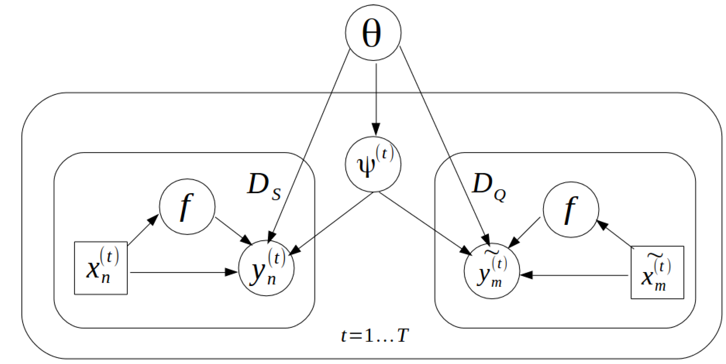
3.1. Probabilistic Model
- initialize
- for , update via (4)
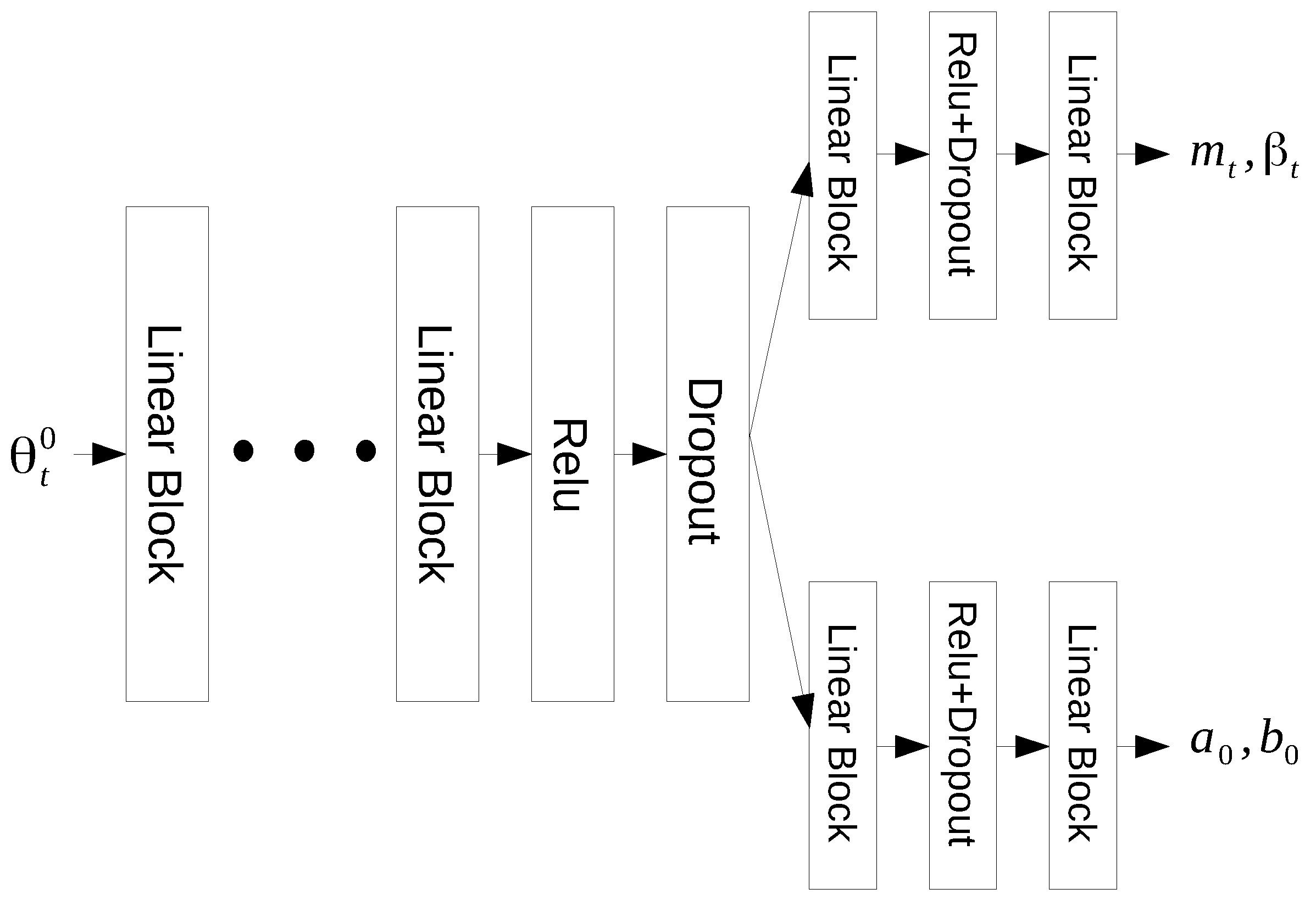
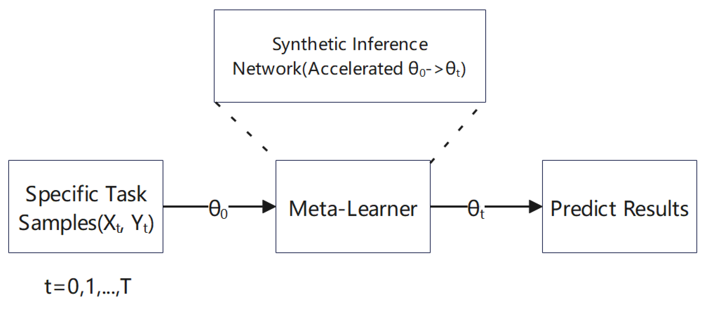
3.2. Fast Transductive Inference with the Synthetic Inference Network
| Algorithm 1 Amortized Bayesian meta-training with SIN. |
|
4. Experiments
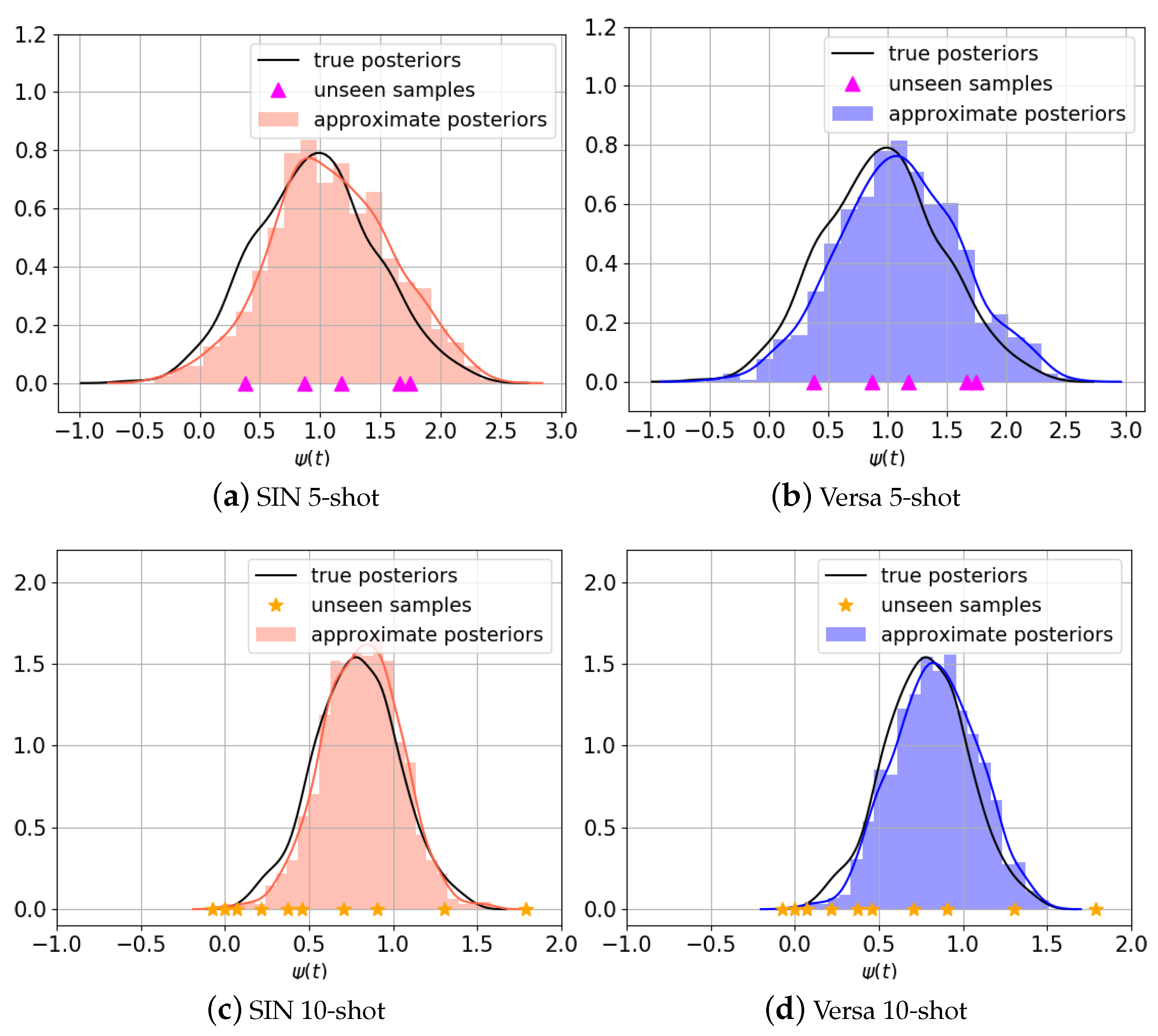
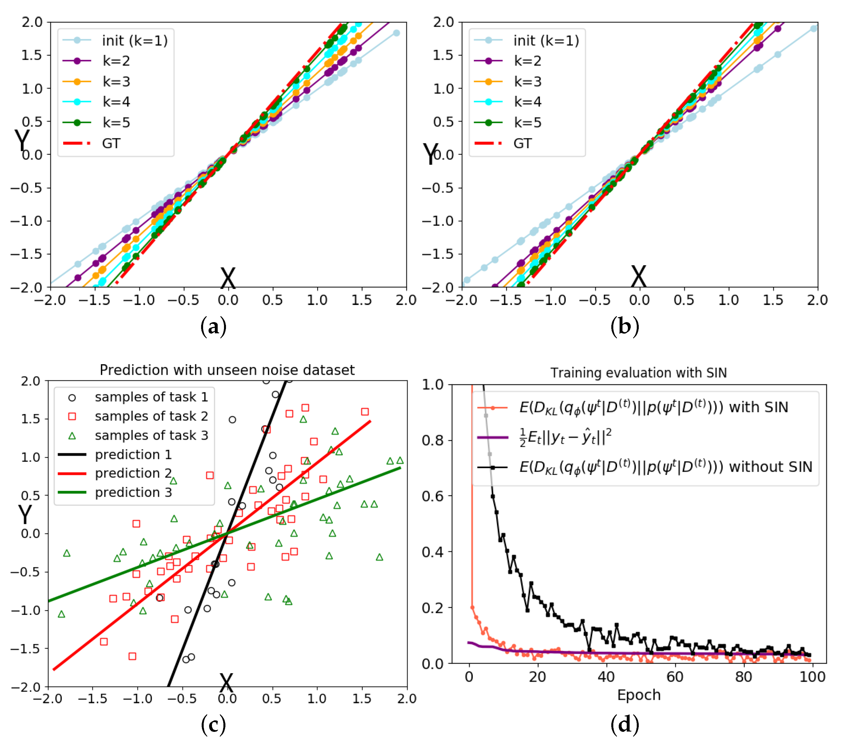
4.1. Data Posterior Inference Examples
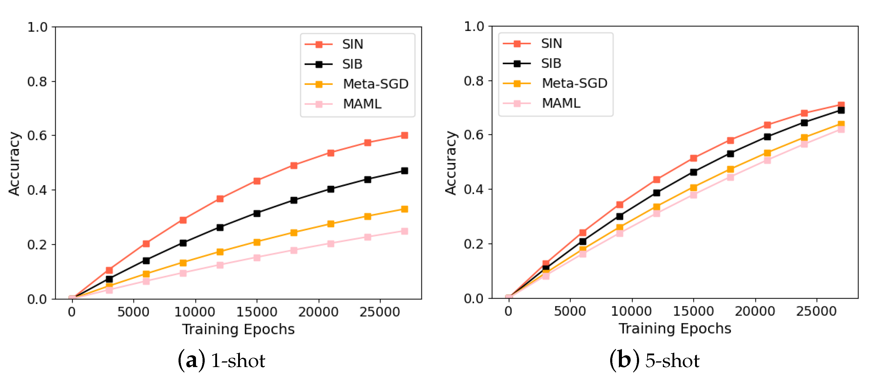
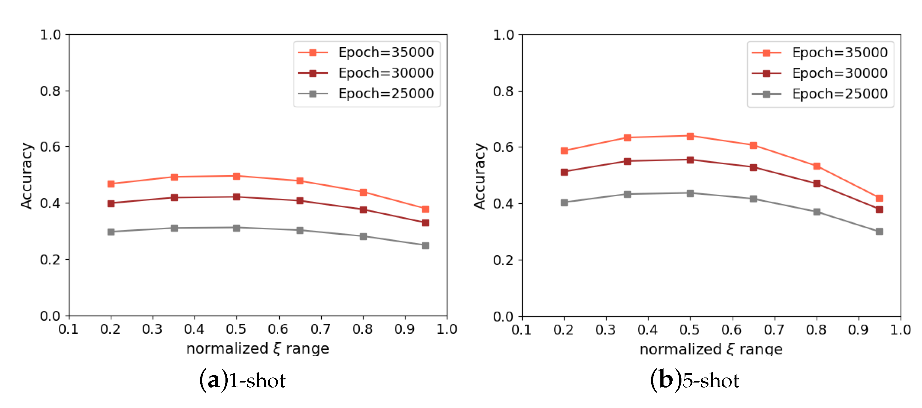
4.2. Mini-ImageNet and Omniglot Dataset Performances
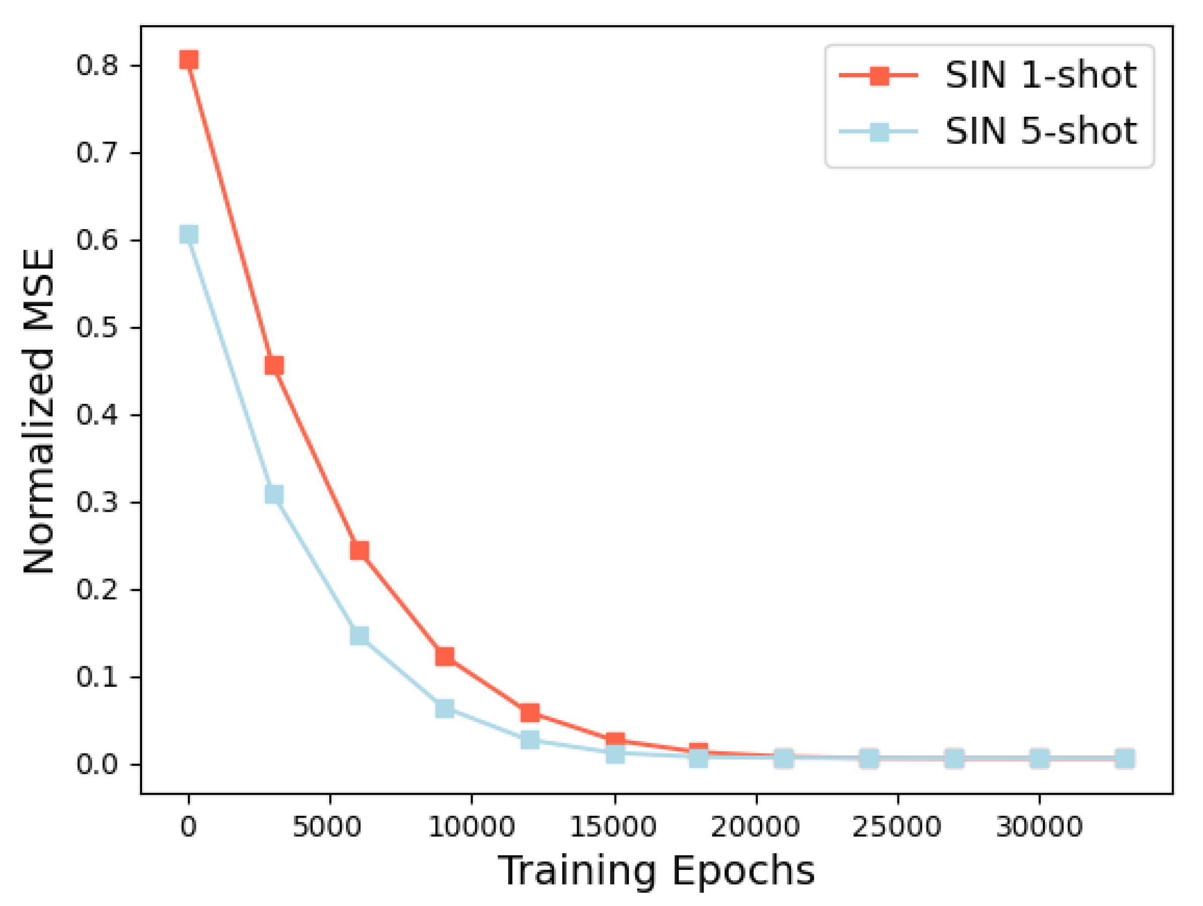
4.3. ShapeNet Dataset View Reconstruction
5. Conclusions
Author Contributions
Funding
Informed Consent Statement
Data Availability Statement
Conflicts of Interest
References
- Li, F.-F.; Fergus, R.; Perona, P. One-shot learning of object categories. IEEE Trans. Pattern Anal. Mach. Intell. 2006, 28, 594–611. [Google Scholar] [CrossRef]
- Ravi, S.; Beatson, A. Amortized Bayesian Meta-Learning. In Proceedings of the ICLR, New Orleans, LA, USA, 6–9 May 2019. [Google Scholar]
- Ravi, S.; Larochelle, H. Optimization as a Model for Few-Shot Learning. In Proceedings of the ICLR, Toulon, France, 24–26 April 2017. [Google Scholar]
- Edwards, H.; Storkey, A. Towards a Neural Statistician. arXiv 2017, arXiv:1606.02185. [Google Scholar]
- Finn, C.; Abbeel, P.; Levine, S. Model-Agnostic Meta-Learning for Fast Adaptation of Deep Networks. In Proceedings of the 34th International Conference on Machine Learning, Sydney, NSW, Australia, 6–11 August 2017; Volume 70, pp. 1126–1135. [Google Scholar]
- Lake, B.M.; Salakhutdinov, R.; Gross, J.; Tenenbaum, J. One shot learning of simple visual concepts. Cogn. Sci. 2011, 33, 2568–2573. [Google Scholar]
- Gordon, J.; Bronskill, J.; Bauer, M.; Nowozin, S.; Turner, R. Meta-Learning Probabilistic Inference for Prediction. arXiv 2019, arXiv:1805.09921. [Google Scholar]
- Louizos, C.; Welling, M. Multiplicative Normalizing Flows for Variational Bayesian Neural Networks. In Proceedings of the 34th International Conference on Machine Learning, Sydney, NSW, Australia, 6–11 August 2017; Volume 70, pp. 2218–2227. [Google Scholar]
- Gal, Y.; Ghahramani, Z. Dropout as a Bayesian Approximation: Representing Model Uncertainty in Deep Learning. In Proceedings of the 33rd International Conference on International Conference on Machine Learning, New York, NY, USA, 19–24 June 2016; Volume 48, pp. 1050–1059. [Google Scholar]
- Amit, R.; Meir, R. Meta-Learning by Adjusting Priors Based on Extended PAC-Bayes Theory. arXiv 2017, arXiv:1711.01244. [Google Scholar]
- Nguyen, C.; Do, T.T.; Carneiro, G. PAC-Bayesian Meta-learning with Implicit Prior and Posterior. arXiv 2020, arXiv:2003.02455. [Google Scholar]
- Hu, S.X.; Moreno, P.G.; Xiao, Y.; Shen, X.; Obozinski, G.; Lawrence, N.D.; Damianou, A. Empirical Bayes Transductive Meta-Learning with Synthetic Gradients. arXiv 2020, arXiv:2004.12696. [Google Scholar]
- Kim, T.; Yoon, J.; Dia, O.; Kim, S.; Bengio, Y.; Ahn, S. Bayesian Model-Agnostic Meta-Learning. arXiv 2018, arXiv:1806.03836. [Google Scholar]
- Finn, C.; Xu, K.; Levine, S. Probabilistic Model-Agnostic Meta-Learning. In Proceedings of the Advances in Neural Information Processing Systems 31: Annual Conference on Neural Information Processing Systems 2018, NeurIPS 2018, Montréal, Canada, 3–8 December 2018; Neural Information Processing Systems Foundation, Inc. (NeurIPS): La Jolla, CA, USA, 2018; pp. 9537–9548. [Google Scholar]
- Vinyals, O.; Blundell, C.; Lillicrap, T.; Kavukcuoglu, K.; Wierstra, D. Matching Networks for One Shot Learning. arXiv 2016, arXiv:1606.04080. [Google Scholar]
- Snell, J.; Swersky, K.; Zemel, R.S. Prototypical Networks for Few-shot Learning. arXiv 2017, arXiv:1703.05175. [Google Scholar]
- Mishra, N.; Rohaninejad, M.; Chen, X.; Abbeel, P. A Simple Neural Attentive Meta-Learner. arXiv 2017, arXiv:1707.03141. [Google Scholar]
- Garnelo, M.; Rosenbaum, D.; Maddison, C.; Ramalho, T.; Saxton, D.; Shanahan, M.; Teh, Y.W.; Rezende, D.; Eslami, S.M.A. Conditional Neural Processes. In Proceedings of the Machine Learning Research, Stockholm, Sweden, 10–15 July 2018; Volume 80, pp. 1704–1713. [Google Scholar]
- Qiao, S.; Liu, C.; Shen, W.; Yuille, A. Few-Shot Image Recognition by Predicting Parameters from Activations. arXiv 2017, arXiv:1706.03466. [Google Scholar]
- Ha, D.; Dai, A.; Le, Q.V. HyperNetworks. arXiv 2016, arXiv:1609.09106. [Google Scholar]
- Gordon, J.; Bronskill, J.; Bauer, M.; Nowozin, S.; Turner, R.E. Decision-Theoretic Meta-Learning: Versatile and Efficient Amortization of Few-Shot Learning. arXiv 2018, arXiv:1805.09921. [Google Scholar]
- Rothfuss, J.; Fortuin, V.; Josifoski, M.; Krause, A. PACOH: Bayes-optimal meta-learning with PAC-guarantees. In Proceedings of the International Conference on Machine Learning, Virtual, 18–24 July 2021; pp. 9116–9126. [Google Scholar]
- Liu, Q.; Wang, D. Stein variational gradient descent: A general purpose bayesian inference algorithm. Adv. Neural Inf. Process. Syst. 2016, 35, 29. [Google Scholar]
- Wang, R.; Sun, H.; Wei, Q.; Nie, X.; Ma, Y.; Yin, Y. Improving Generalization in Meta-Learning via Meta-Gradient Augmentation. arXiv 2023, arXiv:2306.08460. [Google Scholar]
- Wang, L.; Zhou, S.; Zhang, S.; Chu, X.; Chang, H.; Zhu, W. Improving Generalization of Meta-Learning with Inverted Regularization at Inner-Level. In Proceedings of the IEEE/CVF Conference on Computer Vision and Pattern Recognition, Vancouver, Canada, 18–22 June 2023; pp. 7826–7835. [Google Scholar]
- Kingma, D.P.; Welling, M. Auto-Encoding Variational Bayes. arXiv 2013, arXiv:1312.6114. [Google Scholar]
- Garnelo, M.; Schwarz, J.; Rosenbaum, D.; Viola, F.; Rezende, D.J.; Eslami, S.M.A.; Whye Teh, Y. Neural Processes. arXiv 2018, arXiv:1807.01622. [Google Scholar]
- Kingma, D.P.; Ba, J. Adam: A Method for Stochastic Optimization. In Proceedings of the 3rd International Conference on Learning Representations, ICLR 2015, San Diego, CA, USA, 7–9 May 2015. [Google Scholar]
- Mescheder, L.M.; Nowozin, S.; Geiger, A. Adversarial Variational Bayes: Unifying Variational Autoencoders and Generative Adversarial Networks. In Proceedings of the 34th International Conference on Machine Learning, ICML 2017, Sydney, NSW, Australia, 6–11 August 2017; Volume 70, pp. 2391–2400. [Google Scholar]
- Donahue, J.; Krähenbühl, P.; Darrell, T. Adversarial Feature Learning. arXiv 2016, arXiv:1605.09782. [Google Scholar]
- Li, Z.; Zhou, F.; Chen, F.; Li, H. Meta-SGD: Learning to Learn Quickly for Few-Shot Learning. arXiv 2017, arXiv:1707.09835. [Google Scholar]
- Chang, A.X.; Funkhouser, T.; Guibas, L.; Hanrahan, P.; Huang, Q.; Li, Z.; Savarese, S.; Savva, M.; Song, S.; Su, H.; et al. ShapeNet: An Information-Rich 3D Model Repository. arXiv 2015, arXiv:1512.03012. [Google Scholar]
- Zenati, H.; Romain, M.; Foo, C.; Lecouat, B.; Chandrasekhar, V. Adversarially Learned Anomaly Detection. In Proceedings of the 2018 IEEE International Conference on Data Mining (ICDM), Singapore, 17–20 November 2018; pp. 727–736. [Google Scholar]


| Method | Backbone | 1-Shot | 5-Shot | Epochs |
|---|---|---|---|---|
| Matching Nets [15] | Conv-4-64 | 44.2% | 57% | 30,000 |
| MAML [5] | Conv-4-64 | 60,000 | ||
| Meta-SGD [31] | Conv-4-64 | 50,000 | ||
| Prototypical-Nets [16] | Conv-4-64 | 40,000 | ||
| Versa [21] | Conv-5-64 | 60,000 | ||
| SIB [12] | Conv4-4-64 | 50,000 | ||
| SIN (Ours) | Conv4-4-64 | 35,000 |
| Method | Backbone | 1-Shot | 5-Shot | Epochs |
|---|---|---|---|---|
| Matching Nets [15] | Conv-4-64 | 97.3% | 98.6% | 30,000 |
| MAML [5] | Conv-4-64 | 60,000 | ||
| Meta-SGD [31] | Conv-4-64 | 50,000 | ||
| Prototypical-Nets [16] | Conv-4-64 | 40,000 | ||
| Versa [21] | Conv-5-64 | 60,000 | ||
| SIB [12] | Conv4-4-64 | 50,000 | ||
| SIN (Ours) | Conv4-4-64 | 35,000 |
| Output Size | Layers |
|---|---|
| input image | |
| conv2d (, stride = 1, padding = SAME), pool | |
| conv2d (, stride = 1, padding = SAME), pool | |
| conv2d (, stride = 1, padding = SAME), pool | |
| conv2d (, stride = 1, padding = SAME), pool | |
| full connection layer, activation=ReLu | |
| input layer | |
| dense, activation = Tanh | |
| dense, activation = Tanh | |
| full connection layer, activation = ReLu |
| Method | MSE | SSIM |
|---|---|---|
| C-VAE [33] 1-shot | 0.0277 | 0.5923 |
| C-VAE 5-shot | 0.0265 | 0.5639 |
| Versa [7] 1-shot | 0.0108 | 0.7893 |
| Versa 5-shot | 0.0069 | 0.8483 |
| SIN 1-shot | 0.0065 | 0.8492 |
| SIN 5-shot | 0.0061 | 0.8521 |
| Method | Config | Acc (5way-1shot) | Epochs | Training Time | GPU Memory | Model Params |
|---|---|---|---|---|---|---|
| MAML [5] | supp-sz = 1, query-sz = 15 | 31.1% | 20,000 | 1 h 45 min | 1.8 GB | 4.2 MB |
| Versa [21] | supp-sz = 1, query-sz = 15 | 37.5% | 20,000 | 2 h 15 min | 2.1 GB | 15.4 MB |
| SIB [12] | supp-sz = 1, query-sz = 15 | 40.5% | 20,000 | 3 h 21 min | 3.2 GB | 88.1 MB |
| SIN (Ours) | supp-sz = 1, query-sz = 15 | 45.5% | 20,000 | 1 h 03 min | 3.4 GB | 45.2 MB |
| MAML [5] | supp-sz = 2, query-sz = 25 | 44.3% | 35,000 | 3 h 03 min | 2.2 GB | 4.2 MB |
| Versa [21] | supp-sz = 2, query-sz = 25 | 49.1% | 35,000 | 3 h 55 min | 2.4 GB | 15.4 MB |
| SIB [12] | supp-sz = 2, query-sz = 25 | 52.5% | 35,000 | 5 h 49 min | 3.8 GB | 88.1 MB |
| SIN (Ours) | supp-sz = 2, query-sz = 25 | 56.9% | 35,000 | 2 h 22 min | 4.1 GB | 45.2 MB |
Disclaimer/Publisher’s Note: The statements, opinions and data contained in all publications are solely those of the individual author(s) and contributor(s) and not of MDPI and/or the editor(s). MDPI and/or the editor(s) disclaim responsibility for any injury to people or property resulting from any ideas, methods, instructions or products referred to in the content. |
© 2023 by the authors. Licensee MDPI, Basel, Switzerland. This article is an open access article distributed under the terms and conditions of the Creative Commons Attribution (CC BY) license (https://creativecommons.org/licenses/by/4.0/).
Share and Cite
Zhang, Z.; Li, X.; Wang, S. Amortized Bayesian Meta-Learning with Accelerated Gradient Descent Steps. Appl. Sci. 2023, 13, 8653. https://doi.org/10.3390/app13158653
Zhang Z, Li X, Wang S. Amortized Bayesian Meta-Learning with Accelerated Gradient Descent Steps. Applied Sciences. 2023; 13(15):8653. https://doi.org/10.3390/app13158653
Chicago/Turabian StyleZhang, Zhewei, Xuejing Li, and Shengjin Wang. 2023. "Amortized Bayesian Meta-Learning with Accelerated Gradient Descent Steps" Applied Sciences 13, no. 15: 8653. https://doi.org/10.3390/app13158653
APA StyleZhang, Z., Li, X., & Wang, S. (2023). Amortized Bayesian Meta-Learning with Accelerated Gradient Descent Steps. Applied Sciences, 13(15), 8653. https://doi.org/10.3390/app13158653