1. Introduction
With the rapid growth of the number of vehicles in urban areas, cities face numerous challenges, such as traffic congestion and environmental pollution resulting from vehicle emissions. Intelligent Transportation Systems (ITS) can effectively alleviate the above problems and provide many conveniences to people’s lives [
1]. As a primary foundation in advancing ITS, precise traffic prediction plays a critical role in facilitating vehicle allocation, mitigating road congestion, reducing traffic accidents, and optimizing the operational capacity of urban road networks [
2].
Traffic data often exhibit complex and dynamic spatio-temporal relationships [
3], making accurate predictions challenging. In early studies [
4,
5], traffic data were considered as linear time series for analysis, neglecting non-linear temporal relationships. With the advancement of deep learning, Recurrent Neural Networks (RNNs) have proven effective in capturing non-linear dependencies within time series, leading to their widespread application in traffic prediction [
6]. Nevertheless, these methods focus solely on capturing traffic data’s temporal aspects, failing to encompass the intrinsic spatial characteristics. A road’s traffic state is influenced by its historical traffic state and its neighbors. That is to say, the traffic state of a road is significantly correlated with the spatial structure of the road network. Thus, it is necessary to model the spatial correlation among various road nodes in the traffic network [
7]. Some early studies modeled road networks as grids and used Convolutional Neural Networks (CNNs) to capture spatial features [
8]. However, due to the irregularity of traffic roads and the fact that CNN-based methods typically deal with Euclidean structured data, they cannot effectively capture the complex spatial features of urban road networks [
9]. Recently, Graph Neural Networks (GNNs) have gained adequate traction in traffic prediction [
10], providing a more suitable framework for modeling the spatial characteristics of road networks. GNN-based methods consider each road segment in the road network as a node in the graph [
11,
12], while the relationships between different road segments are treated as edges. This way, the road network is constructed as a structured graph.
While most GNN-based methods have shown promising results, they often rely on predefined static adjacency matrices that cannot effectively capture the complex and dynamically changing spatial dependencies in traffic data. Some methods also extract spatial features by constructing adaptive graph structures [
12,
13], where the model generates the adjacency matrix through learning. However, the adaptive and predefined adjacency matrices remain static, limiting their ability to capture the dynamic spatial dependencies. In real-life scenarios, each road node in a road network can have varying effects on the traffic state of its neighboring road nodes over time. The correlations between road segments are dynamically changing.
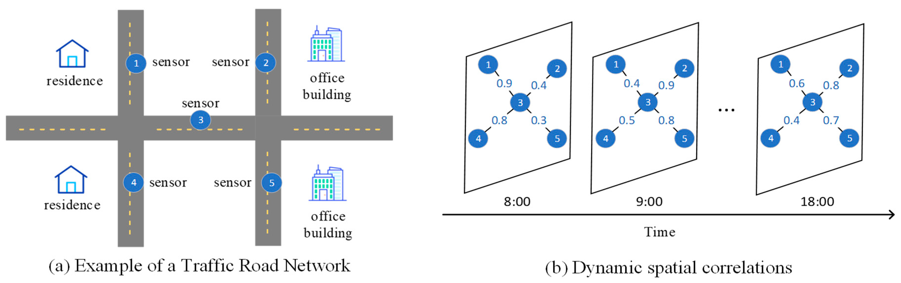
Figure 1a illustrates a traffic road network instance where sensors are strategically placed on the primary roads to record traffic speed data. Sensor 1 and Sensor 4 record the vehicle speeds on roads within residential areas, while Sensor 2 and Sensor 5 record the vehicle speeds on roads within the office area. Sensor 3 is located on a road that lies between these two areas. These sensors are abstracted as nodes in the graph, and the strength of spatial correlation between them is abstracted as edges. As time progresses, the traffic states on various road segments change, and the spatial correlation between road nodes also varies.
Figure 1b illustrates the dynamic changes in correlation between nodes. During the morning peak hours, the traffic states in the residential area significantly affect Sensor 3, but the influence gradually diminishes over time.
Furthermore, existing models commonly employ RNN-based methods or CNN-based methods to model temporal correlations [
14,
15]. RNNs capture temporal dependencies in time series effectively. However, due to the typical sequential structure of RNNs, RNN-based methods require multiple iterations to model long-term temporal correlations, which can lead to error accumulation and gradient explosion issues [
16]. Unlike RNNs, CNN-based methods have advantages such as parallel operations and gradient stabilization. However, CNNs perform implicit temporal modeling. The time steps are not visible, which leads to a lack of flexibility [
17]. Several research studies have employed Transformer-based architectures to extract the temporal dependencies [
18,
19]. These approaches have demonstrated promising capabilities in modeling long-term temporal correlations. However, Transformers rely on positional encoding to capture the order information within a sequence, which leads to limited effectiveness in capturing local temporal correlations [
20].
Considering the multifaceted aspects and complexities of the matter at hand, we propose a method named DSTGFCN based on an encoder–decoder framework to achieve traffic prediction. In particular, the DSTGFCN captures dynamic spatio-temporal features from observed data to construct dynamic adjacency matrix. With the graph convolution gated recurrent network and the dynamic adjacency matrix, the model achieves simultaneous modeling of dynamic spatio-temporal correlations and adds residual connections between the graph convolution gated recurrent layers to address problems such as error accumulation and gradient explosion. The main contributions of this paper can be summarized as follows:
A multi-step ahead prediction model is proposed to achieve accurate traffic prediction. A dynamic graph fusion module can extract spatial information from observed data without prior knowledge and fuse dynamic spatial features from adjacent time steps to generate a dynamic adjacency matrix.
We effectively modeled the dynamic spatio-temporal correlations by combining the Graph Convolutional Gated Recurrent Unit (GC-GRU) with the dynamic adjacency matrix. Residual connections were added between the GC-GRU layers to propagate gradients and extract long-term temporal dependencies efficiently.
The proposed model was tested against multiple baselines on six real-world traffic datasets and showed superior predictions. In addition, ablation experiments validated the effectiveness of each component.
This paper is organized as follows:
Section 2 presents a comprehensive review of related works.
Section 3 introduces the preliminary content and formulates the research problem. Next, in
Section 4, we provide a detailed description of our proposed approach. The experiments, including comparative experiments, ablation experiments, and visualization of predictions, are presented in
Section 5.
Section 6 discusses the advantages of the proposed method. In the end,
Section 7 summarizes the paper and presents plans.
2. Related Work
In the past decades, traffic prediction has been an essential component of ITS and has been extensively researched. Earlier research efforts were usually based on statistical methods for traffic prediction, ignoring the nonlinear characteristics and complex variations in traffic data [
4]. Machine learning methods can capture the nonlinear dependencies in traffic data compared to statistical methods [
5]. However, they rely on high-quality manual features, which can be time-consuming to extract.
With the continuous development of traffic big data and artificial intelligence technologies [
21], a growing body of research has proposed various spatio-temporal modeling methods to capture the spatio-temporal features within traffic data [
7]. Existing approaches usually model traffic data’s temporal and spatial dimensions separately [
22]. Sequence models are typically used to extract temporal relationships, such as Long Short-Term Memory (LSTM) [
23], Gated Recurrent Units (GRUs) [
24], and Temporal Convolutional Networks (TCNs) [
25]. As traffic road networks naturally possess a non-Euclidean structure, GNN-based approaches are well suited for capturing the non-Euclidean relationships between multiple traffic time series to model spatial dependencies [
26]. For instance, the Temporal Graph Convolutional Network (T-GCN) leverages graph convolutional networks (GCNs) to capture spatial features and GRUs to capture temporal features, which can effectively model spatio-temporal correlations [
27].
Recent research has highlighted the limitations of predefined adjacency matrices in adequately capturing the spatial relationships and latent information between nodes when designing spatio-temporal GNNs. The Adaptive Graph Convolutional Recurrent Network (AGCRN) addresses this issue by learning specific node attributes and constructing adaptive graphs to explore latent spatial relationships further [
13]. Similarly, Ta et al. [
28] adopted a macroscopic and microscopic perspective to learn global and local spatial structures, aiming to acquire an optimal graph structure. Jiang et al. [
29] proposed a Meta-Graph Learner that relies solely on observed data to construct an adaptive adjacency matrix. The abovementioned methods have further improved prediction accuracy in traffic forecasting tasks, indicating that adaptive adjacency matrices can compensate for the limitations of predefined adjacency matrices in modeling spatial correlations. However, in traffic data, the spatial relationships among road segments are vary with time. Li et al. [
17] designed a dynamic graph generator that extracts static, dynamic, and temporal information from traffic data to generate dynamic graphs. Zhao et al. [
30] employed a channel attention mechanism to allocate dynamic weights to historical traffic sequences at different time steps to achieve dynamic adjustment of spatio-temporal correlation. In the work of Hu et al. [
31], dynamic graphs were generated by combining spatial heterogeneity information and geospatial proximity information at each time step. Zhang et al. [
32] modeled dynamic spatial correlations by exploring fine-grained features between nodes. Zheng et al. [
33] concatenated spatial information from recent time steps and each past time step to generate dynamic spatio-temporal graphs. Despite achieving promising predictive performance, the above methods rely on prior road spatial knowledge and fail to effectively extract dynamic features from traffic data and model dynamic spatial correlations.
Motivated by the abovementioned research, we propose a novel traffic prediction model called DSTGFCN. This model addresses the challenges of complex and dynamic road networks by extracting dynamic spatial information from observed data and generating a dynamic adjacency matrix at each time step, all without relying on prior knowledge of the road spatial relationships. Therefore, DSTGFCN is not limited to a fixed spatial structure and applies to large-scale traffic road networks.
4. Methodology
The overall framework of the proposed DSTGFCN is shown in
Figure 2. This framework employs an encoder–decoder structure to facilitate multi-step prediction. Inspired by the research in [
13], we substituted all the linear layers in the GRU with graph convolutions to construct GC-GRU as the fundamental unit for spatio-temporal modeling. During the encoding stage, the dynamic graph fusion module extracts spatial information for each time step based on the traffic state, time information, and learnable spatial node embeddings to model dynamic spatial correlations. Then, it fuses the dynamic spatial features of adjacent time slots to generate a dynamic graph. The GC-GRU receives the dynamic adjacency matrix to model dynamic spatio-temporal correlations. Simultaneously, the spatial node embeddings adequately learn the dynamic and latent spatial information from historical traffic data to construct an adaptive adjacency matrix. Since future traffic states cannot be observed during the decoding phase, the decoder utilizes an adaptive adjacency matrix to model spatio-temporal correlations and achieve multi-step traffic prediction. Furthermore, residual connections are added between layers of the GC-GRU to harness the capacity of the multi-layer network in a stable training process.
4.1. Dynamic Graph Fusion Module
In this section, we will design a dynamic graph fusion module. This module aims to generate an adjacency matrix that represents the dynamic spatial correlations in the traffic road network by fusing the dynamic features extracted from the road attributes. As the dynamic spatio-temporal correlations heavily depend on real-time traffic states, it is essential to model the dynamic spatial correlations by inputting real-time traffic states.
The core of constructing the dynamic feature matrix ensures a comprehensive encoding of the input’s dynamic, latent spatial, and temporal information. To achieve this, we incorporate the following components at each time step: the current traffic state
, and the time-related embeddings including time of day
and day of the week
. To further efficiently extract the hidden space features between nodes, we use two spatial node embeddings
and
. Additionally, we extract features for the traffic state
using two non-linear fully connected layers and convert the dimensionality from
to
. From this, at time step
, we create two dynamic feature matrices by fusing the above features in a concatenated manner as follows:
where
,
is the number of nodes,
is the feature dimension,
is the node embedding dimension, and
is the temporal embedding dimension.
denotes the network of two non-linear fully connected layers. We then compute the dynamic feature matrix at the current time step using the self-attention mechanism [
34]:
where
are the parameters of the self-attention mechanism.
denotes the spatial correlation between road nodes at time step
. In this way, each dynamic feature matrix can learn unique adjacency relationships at each input time step through Equation (4), which reflects the time-varying traffic topology.
Although the traffic conditions are dynamic, these changes occur gradually. For instance, the relationships between neighboring road segments exhibit variations during peak and off-peak periods. However, within consecutive time intervals, the local spatial dependencies between neighboring road segments change slowly. Hence, we employ a gating mechanism to extract and fuse crucial spatial topological information from the current time step’s dynamic feature matrix
and the previous time step’s dynamic adjacency matrix
, as follows:
where
are two learnable linear transformation matrices. Finally, we can obtain the dynamic adjacency matrix
at time step
:
The dynamic graph fusion module combines the dynamic spatial information of the road network at each time step to generate the dynamic adjacency matrix. However, during the decoding phase, future traffic states cannot be observed, and the input to each GC-GRU in the decoder is the previous time step’s predicted output. Using predicted outputs to construct the dynamic adjacency matrix may introduce errors and inaccurately represent the road network structure. In the encoding stage,
and
implicitly learn the dynamic and latent features from historical information through the dynamic graph fusion module. Therefore, we utilize
and
to construct an adaptive adjacency matrix in the decoder to represent the spatial structure:
During the decoding and prediction phase, the adaptive adjacency matrix can effectively extract spatial dependencies within the road network through graph convolution.
4.2. Graph Convolutional Gated Recurrent Layer
The spectral-based GCN has shown great potential in capturing spatial correlations among traffic sequences [
35,
36]. Given the traffic road nodes, the GCN is a fundamental operation for extracting features from these nodes. The graph convolution operation is approximated using a first-order Chebyshev polynomial expansion as follows:
Here,
and
are the input and output of the graph convolution operation
.
is the adjacency matrix,
is the degree matrix, and
and
denote the learnable weight and bias, respectively. However, Equation (8) only considers the effect of first-order neighboring nodes. According to the summary and analysis of Yin et al. [
37], we employ a diffusion convolution layer to model the graph signal’s diffusion process within
finite steps. Thus, for Equation (8), we utilize the diffusion convolution in the following manner:
Besides spatial correlation, traffic prediction is also influenced by complex temporal correlation. The GRU has gained popularity and has been extensively applied in time series prediction. Similar to previous works [
18], we combined the diffusion graph convolution and GRU modules and refer to them as the GC-GRU. As illustrated in
Figure 3, the GC-GRU replaces the linear layers responsible for the gating and update gates in the GRU with the graph convolution. As a result, the GC-GRU can effectively model both temporal and spatial correlations in the input graph signal, as shown in the following equation:
At time step , represents the input and represents the output hidden state of GC-GRU. and denote the update gate and reset gate. The notation denotes the diffusion graph convolution operation defined by Equation (10), and are the learnable parameters corresponding to the diffusion graph convolution. denotes the Hadamard product.
Although the GRU addresses the issue of vanishing gradients in RNNs during backpropagation, it cannot retain all the information for long durations. In a multi-layer GRU, the lower layers can capture local temporal dependencies, while higher layers can capture longer-range temporal dependencies. However, using multiple layers of GRU during training can lead to problems like vanishing or exploding gradients. Residual connections mitigate the decay of gradients during the propagation between layers. Adding residual connections in multi-layer GRUs can alleviate the vanishing or exploding gradient issues, making the training process more stable. As shown in
Figure 2, DSTGFCN adopts two layers of GC-GRU in both the encoder and decoder to enhance the model’s ability to extract spatial and temporal features in long-term prediction scenarios. The
units (corresponding to
historical time steps) form a graph convolution gated recurrent layer in a cascading manner, and residual connections are added between the layers to enhance the model’s prediction capability and stability.
4.3. Multi-Step Traffic Prediction
In
Figure 2, the decoder module is employed for multi-step traffic prediction. It utilizes the hidden states from the encoder and the adaptive graph adjacency matrix obtained from the dynamic graph structure learning module to recursively generate multi-step predictions, i.e., the future traffic state.
loss is selected as the loss function:
Here, denotes all trainable parameters in the model, is the count of prediction steps, and is the quantity of road nodes. and represent the prediction and ground truth of node at time .
5. Experiments
Next, we conducted experiments on six real-world datasets to demonstrate the effectiveness of DSTGFCN in traffic speed or flow prediction tasks. In this section, we will first introduce the datasets, experimental settings, evaluation metrics, and representative baselines. Next, we will discuss the experiments comparing the performance of DSTGFCN against other baselines. Furthermore, we conducted ablation experiments to assess the impact of individual components in the model on predictive performance. Finally, we will visualize the predicted values and dynamic adjacency matrix for a more intuitive understanding and evaluation of the model.
5.1. Datasets
We evaluated the performance of our model using six real-world traffic datasets, which encompass two types of traffic data: traffic speed and traffic flow.
METR-LA is a dataset of traffic speed collected from 207 sensors on the highways in Los Angeles.
PEMS-BAY is a dataset comprising traffic speed data from 325 traffic road sensors in the Bay Area.
PEMS03 is a dataset of traffic flow collected from 358 sensors in the California Third District.
PEMS04 is a dataset of traffic flow collected from 307 San Francisco Bay Area sensors.
PEMS07 is a dataset of traffic flow collected from 883 sensors in the California Seventh District.
PEMS08 is a dataset composed of traffic flow data collected from 170 sensors in the San Bernardino area.
Table 1 presents the detailed information on these six datasets. Following previous research works [
12,
38], we divided the first two traffic speed datasets into training, validation, and testing sets in a ratio of 7:1:2. The division ratio was 6:2:2 for the other traffic flow datasets. All data points were collected every 5 min. Z-score normalization was used to standardize all the datasets.
We analyzed the six datasets mentioned above, as shown in
Figure 4. For the traffic speed datasets, we display the distribution of speed values. The METR-LA dataset exhibits some extreme values, which can be attributed to missing data. In contrast, the speed distribution in the PEMS-BAY dataset was concentrated between 50 mph and 80 mph, indicating a relatively simple traffic pattern with less congestion. We illustrated the distribution of flow values of these traffic flow datasets. PEMS03, PEMS04, and PEMS08 displayed similar flow distributions, with traffic flow concentrated between 0 and 300 vehicles per hour. In contrast, the flow distribution in the PEMS07 dataset was more uniform, lacking clear traffic patterns.
5.2. Experiment Settings
All experiments were performed on a computer with an Intel Core i9 13900K/F
[email protected] GHz and a GeForce RTX 3090 GPU card with 24 G of video memory, and the model was implemented based on the PyTorch 1.12.0 framework. The number of hidden states was 32. The time and node embedding dimension were 15 and 20, respectively. Both the historical observation and prediction data steps were set to 12. We used the Adam optimizer to optimize the model, where the learning rate was set to 0.01, and batch size was set to 32. The optimization time was 100 epochs, and early stopping was employed to avoid overfitting.
5.3. Evaluation Metrics
The experiment used three metrics that are widely used to assess the accuracy of traffic prediction, which are Mean Absolute Error (MAE), Root Mean Square Error (RMSE), and Mean Absolute Percentage Error (MAPE). The details of the equations are as follows:
Among them, MAE is the average of the absolute errors between the predicted values and the ground truth, reflecting the prediction accuracy. RMSE measures the concentration of prediction results around the line of best fit. MAPE reflects the relative magnitude of the deviations between the predicted values and the ground truth. is the number of samples. and denote the ground truth and the predicted values of the sample. Smaller values indicate better prediction performance for the above three metrics.
5.4. Baseline Methods
We compared DSTGFCN with eight baselines, including a traditional time series analysis method (ARIMA), deep learning-based methods (FC-LSTM, STGCN, and DCRNN), and excellent existing GNN-based methods (GW-net, AGCRN, DSTAGCN, and STG-NCDE).
ARIMA [
14]. A statistical model commonly used for analyzing and predicting time series data.
FC-LSTM [
14]. LSTM network with the fully connected network to generate traffic series predictions.
STGCN [
11]. This model employs graph convolution and 1D convolution to capture spatial and temporal features, respectively.
DCRNN [
14]. DCRNN combines dual directional diffusion convolution and GRUs for traffic prediction.
GW-Net [
12]. Graph WaveNet combines diffusion causal convolution with GCNs based on an adaptive adjacency matrix to capture potential spatial correlations.
AGCRN [
13]. The model captures spatial correlations between roads through the two proposed adaptive learning modules.
DSTAGCN [
33]. The model connects multiple time frames to construct a dynamic spatio-temporal graph, capturing global spatio-temporal correlations.
STG-NCDE [
39]. The model employs two neural control differential equations to forecast traffic states.
5.5. Experimental Results and Comparative Analysis
Table 2 presents the performance comparison between DSTGFCN and the baseline models for 15 min (short-term), 30 min (mid-term), and 60 min (long-term) predictions on the METR-LA and PEMS-BAY datasets.
Table 3 displays the performance comparison between DSTGFCN and the baseline models for average one-hour predictions on the four traffic flow datasets. Our proposed model demonstrated superior predictive performance in traffic speed and traffic flow prediction tasks. The traditional statistical method ARIMA performed the worst, failing to capture the nonlinear relationships in the traffic sequences. FC-LSTM, being a classical recurrent neural network, effectively extracted nonlinear features from sequences. However, it only modeled temporal correlations and overlooked the spatial correlations in the traffic road network, resulting in lower accuracy than the graph-based models. This finding highlights the importance of modeling spatial correlations to achieve accurate predictions.
STGCN and DCRNN are typical spatio-temporal data prediction models. Both models consider spatial factors, which lead to improved prediction accuracy. However, these methods only utilize adjacency matrices defined by spatial distances for graph convolution operations, which may only partially capture spatial relationships. GW-Net, AGCRN, and STG-NCDE employ adaptive adjacency matrices to explore further hidden spatial features, which can be understood as learning the optimal graph topology of the traffic road network. Although they demonstrated excellent performance, these models still employed static graphs when modeling spatial correlations and did not consider the dynamic variations of spatial relationships. DSTAGCN connects the graphs of the recent and past time frames to construct a dynamic adjacency matrix, resulting in improved prediction capabilities compared to static graphs. Compared to the models above, DSTGFCN fully extracted the dynamic features from the traffic data and combined dynamic spatial features from multiple time frames to generate the dynamic adjacency matrix more efficiently and appropriately. As a result, DSTGFCN exhibited excellent predictive capabilities.
Figure 5 visualizes the prediction errors of DSTGFCN and two other baselines at each time step on the PEMS04 and PEMS08 datasets. The error growth rates of AGCRN and STG-NCDE were similar, but STG-NCDE performed better than AGCRN in short-term predictions. AGCRN exhibited good performance in long-term predictions on the PEMS08 dataset, where DSTGFCN slightly lagged behind AGCRN regarding MAPE. However, overall, DSTGFCN demonstrated lower errors across the entire time range, showcasing the superior performance of our model.
Lastly, we found that the difficulty of prediction varied across different datasets. Traffic flow data exhibited a more comprehensive range of variations than traffic speed data, as traffic speed is usually constrained within a specific speed range. Therefore, traffic flow data are more complex, leading to more significant errors for all models in traffic flow prediction tasks. In
Figure 4, the PEMS-BAY dataset shows a relatively simple traffic pattern, resulting in significantly better prediction results. However, in contrast, the PEMS07 dataset exhibits a more complex traffic pattern, leading to larger MAE and RMSE values for all models on that dataset. Consistently achieving better prediction results across all the datasets demonstrated that DSTGFCN effectively captures the dynamic spatio-temporal dependencies in the traffic road network. This allows DSTGFCN to demonstrate outstanding performance in both traffic speed and traffic flow prediction tasks.
5.6. Ablation Experiments
We conducted ablation experiments to validate the effectiveness of each component in the proposed DSTGFCN model. All ablation experiments were performed on the METR-LA dataset. We named the variants of DSTGFCN as follows:
w/o Dg: We replaced the dynamic adjacency matrix in DSTGFCN with a predefined adjacency matrix. That is, dynamic graph fusion was also removed. The predefined adjacency matrix was constructed in reference to the way defined by Li et al. [
14]. The calculation formula is as follows:
where
represents the road network distance from sensor node
to
.
is the standard deviation of the distance and
is the threshold value, which was assigned a value of 0.1.
w/o Fus: We removed dynamic graph fusion when building the dynamic graphs.
w/o Res: We removed the residual connections in the graph convolution gated recurrent layer.
w/o Fus & Res: We removed both dynamic graph fusion and the residual connections.
Dg2Sg: DSTGFCN replaced the dynamic adjacency matrix with a predefined adjacency matrix while removing dynamic graph fusion and the residual connections.
Dg w/o X: Traffic states are not considered as input when constructing the dynamic graph.
Dg w/o T: Time embedding was not considered as input when constructing the dynamic graph.
Dg w/o E: Node embedding was not considered as input when constructing the dynamic graph.
As shown in
Table 4, we can observe that DSTGFCN outperformed other variants in terms of prediction accuracy for 15 min, 30 min, and 60 min. Analysis of the results indicates a significant decline in predictive performance when the dynamic adjacency matrix was removed (w/o Dg, Dg2Sg). Therefore, it is necessary to construct a dynamic adjacency matrix to capture dynamic spatio-temporal features effectively. Additionally, dynamic graph fusion further enhanced the prediction performance (w/o Fus), validating that the adjacency relationships of road nodes exhibit certain similarities in adjacent time steps. The residual connections improved the model’s ability to capture long-term dependencies. Specifically, in 60 min predictions, DSTGFCN achieved an MAE reduction from 3.45 to 3.28 compared to DSTGFCN w/o Res, resulting in a 4.92% improvement in prediction accuracy. Meanwhile, DSTGFCN w/o Fus & Res validated that only considering the dynamic adjacency matrix is inadequate for accurate prediction. Ablation experiments on the input of dynamic feature extraction indicate that the deficiencies in the current traffic state (Dg w/o X), time embedding (Dg w/o T), and node embedding (Dg w/o E) will lower the prediction performance. In summary, these components are all crucial for the prediction performance of DSTGFCN.
5.7. Visualization
To further visually understand and evaluate the proposed model in this paper, we visualized the ground truth and the model’s predictions. As shown in
Figure 6, we selected two nodes from the METR-LA dataset, Node 89 and Node 101, and displayed their data for an entire day on 11 June 2012 (from the test set). These two nodes displayed distinct traffic patterns. For example, Sensor 89 showed traffic congestion only during the morning peak hours, while Sensor 101 experienced traffic congestion not only during the morning peak hours but also during the evening peak hours. The results indicate that DSTGFCN can capture different traffic patterns of different nodes. Additionally, we can observe that the ground truth curves were highly irregular with significant fluctuations. Our model could effectively adapt to these abrupt trend changes and make predictions that closely approximate the ground truth as much as possible. However, specific local details in the predictions may be less accurate due to random solid noise, such as the sudden and significant fluctuations during the morning peak hours in
Figure 6a.
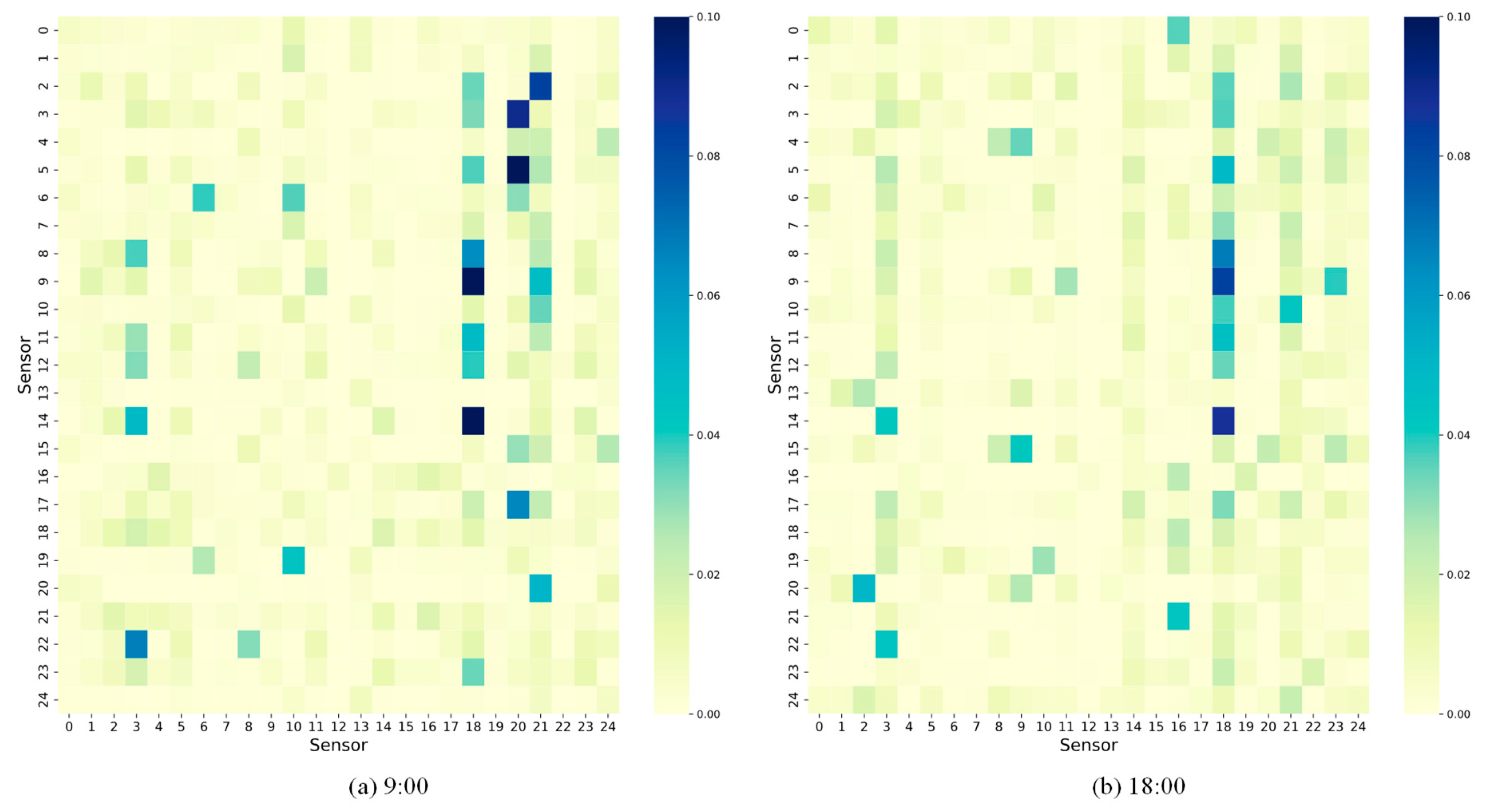
To visually observe the dynamic spatial correlations in the traffic road network, we selected 25 nodes from the METR-LA dataset. We visualize their dynamic adjacency matrices for two time periods in
Figure 7. It can be observed that the dynamic adjacency matrices changed over time. For instance, Node 20 and Node 5 exhibited a strong correlation at 9:00, but their correlation weakened at 18:00. Additionally, Node 18 showed a similar correlation with other nodes in both periods. This indicates that specific road segments have similar traffic patterns during peak hours. These findings demonstrate that DSTGFCN effectively constructs dynamic adjacency matrices to capture the dynamic topological relationships in the traffic road network.


