All articles published by MDPI are made immediately available worldwide under an open access license. No special
permission is required to reuse all or part of the article published by MDPI, including figures and tables. For
articles published under an open access Creative Common CC BY license, any part of the article may be reused without
permission provided that the original article is clearly cited. For more information, please refer to
https://www.mdpi.com/openaccess.
Feature papers represent the most advanced research with significant potential for high impact in the field. A Feature
Paper should be a substantial original Article that involves several techniques or approaches, provides an outlook for
future research directions and describes possible research applications.
Feature papers are submitted upon individual invitation or recommendation by the scientific editors and must receive
positive feedback from the reviewers.
Editor’s Choice articles are based on recommendations by the scientific editors of MDPI journals from around the world.
Editors select a small number of articles recently published in the journal that they believe will be particularly
interesting to readers, or important in the respective research area. The aim is to provide a snapshot of some of the
most exciting work published in the various research areas of the journal.
The protection of structures and machines from ground vibrations is a deeply felt and widely studied problem. These vibrations are typically generated by the operation of machines, vehicular traffic, seismic events, shocks, explosions, etc., and are generally characterized by frequencies that are not known a priori, making the use of passive isolation systems problematic. Just away from the source, ground vibrations have a predominantly horizontal component. To meet the conflicting requirements of passive isolation systems, which should have higher stiffness when the structure is at rest and lower stiffness when the ground forces it to vibrate, active or semi-active isolation systems can be adopted. In the following article, the possibility of adopting a hybrid isolator is evaluated; it consists of shear-stressed elastomeric pads coupled with an electromagnetic actuator; the latter consists of three coils, two of which are connected to the ground and the other one to the body to be isolated. This kind of isolator has the same flexibility and adaptability as the active ones, with the advantage of ensuring its functioning even in the absence of an external energy source. Its flexibility is due to the presence of a smart element that allows one to tune the characteristics of the isolator to consider the instantaneous isolation requirements. The proposed solution allows one to modify the isolation system’s characteristics in a sufficiently wide range of displacements equal to that defined by the maximum allowed deformation of the elastomeric pads. This paper reports the description of the isolation system and an analytical model to describe its restoring force; then, an experimental setup is adopted to identify the parameters of the analytic model; finally, several simulations are reported to compare the analytical and the experimental trends of the restoring force and to characterize the isolator.
Passive vibration isolators are a simple and effective way to protect structures and machines from vibrations if the forcing frequency is known a priori; they are also reliable as they do not require a power supply, which may not be available when it is needed. Linear vibration theory shows that an isolator is effective if the forcing frequency is greater than , where is the natural frequency of the isolated system; therefore, to increase the isolation frequency range, a less stiff isolator system should be adopted, but this choice could lead to excessive displacements. Therefore, an insulation system often has two conflicting requirements: in the case of vertical excitation, the isolation system must be sufficiently stiff to support the structure’s weight, while it should be flexible enough to provide low transmissibility. In the case of horizontal excitation, it should be stiff enough to prevent any small actions from causing large displacements, but it should also be sufficiently compliant to isolate vibrations. Therefore, in many cases, the linear-elastic theory does not allow the problem of vibration isolation to be solved, and some solutions can be obtained by adopting passive isolators with nonlinear behavior or by adopting active/semi-active isolation systems that allow the adjustment of the restoring force according to the state of the isolated body.
Low natural frequencies can be achieved by adopting passive isolators such as air springs or wire rope springs. The stiffness of air springs [1,2] mainly depends on the air volume and pressure. Their behavior has been extensively studied in the field of vehicle suspensions, where they allow the vehicle attitude to be kept constant as the mass of the suspended body varies. They are often used in combination with a damper due to their low level of damping.
Wire rope springs [3,4,5] have hysteretic nonlinear behavior depending on the length–diameter ratio of the ropes and on the spring configuration. The restoring force depends on the instantaneous and past deformation. They are characterized by a good level of damping due to the friction forces developed between the wires of the rope. These kinds of isolators combine a high level of isolation while taking up relatively little space; they are made of stainless steel and therefore do not suffer the attack of external factors (atmospheric agents, oils, etc.).
Although both types of insulators can achieve sufficiently low natural frequencies, they may not achieve adequate isolation if the forcing frequency is not known in advance. If the forcing frequency is close to the resonance condition, the amplification of the transmissibility can be avoided only through an adequate increase in the damping of the isolation system, but this solution worsens the transmissibility for higher forcing frequencies.
A significant nonlinear passive device was proposed by Molineux [6] in 1957 (Figure 1a) in the case of vertical excitation; it consists of two equally inclined springs (k1) combined with a vertical spring (k2). The vertical reaction of the two inclined springs decreases with the displacement until it becomes zero when their axes are aligned in the horizontal direction; beyond this configuration, the set of the two inclined springs provides a negative restoring force, as shown in Figure 1b, for k2/k1 = 0. Thanks to the presence of the k2 spring, the device provides a restoring force whose nonlinear trend depends on the ratio k2/k1; with increasing k2 stiffness, the restoring force becomes positive, and for further increments, its trend becomes monotonic (e.g., for k2/k1 = 0.5 in Figure 1b) with a range of displacements characterized by a low equivalent vertical stiffness. In this case, the springs may be sized so that a low stiffness range is reached at the static equilibrium condition with the advantage that the weight involves low displacements thanks to the greater initial stiffness and that, at the equilibrium position, the vertical stiffness (and therefore the vibration transmissibility) is low. Isolators with these characteristics are indicated with the acronym HSLDS (high-static, low-dynamic systems) or QZSS (quasi-zero-stiffness systems) if, in the position of static equilibrium, the stiffness assumes a value of almost zero.
Molyneux’s experience shows that the combination of a negative-stiffness device with a positive one leads to a device with a nonlinear force–displacement relationship and that, if the ratio between the stiffnesses is appropriately chosen, the device can exhibit stability, small static deformation, and high damping ratio as the potential energy produced by a negative stiffness device is negative, which means a loss of energy along with deformation. These characteristics can be conveniently exploited for the mitigation of vibrations. The dynamic behavior of this type of isolator supporting a lumped mass can be approximately described by the Duffing equation [7]. An isolator based on this principle is proposed in [8] to protect structures from vertical seismic accelerations.
Low dynamic stiffness isolators have received considerable attention as this isolation technique allows the transmissibility to be reduced by coupling a negative-stiffness device with a positive-stiffness one, as reported in an interesting review in [9]. These devices can be made in different ways, such as by means of inclined springs, buckled beams, and scissor-like mechanisms involving geometric nonlinearities [10]. However, these mechanisms have some drawbacks that limit their application; for example, pre-stressed inclined springs exhibit negative stiffness only when the displacement exceeds a certain limit; buckled beams exhibit an asymmetrical negative stiffness near the equilibrium point; furthermore, they exhibit good performances only close to the nominal operating conditions.
Passive isolators are activated by the relative motion between the isolated body and its support; they are preferred to semi-active/active isolators for their simplicity and when it is feared that the external energy contribution may not always be available.
Semi-active isolators can be considered passive devices in which it is possible to adjust a rheological property (damping or stiffness) in real time to adapt it to the needs of the isolation. Unlike active systems, they cannot feed energy into the controlled system and are often preferred to active ones as they require less energy and can operate with lower efficiency, even in the absence of external energy. A popular type of semi-active insulator consists of a spring coupled with a magnetorheological damper [11] whose damping can be adjusted in real time. Another type of semi-active isolator is based on the use of magnetorheological rubbers whose properties are shown in [12], and the possibility of controlling their stiffness is explained in [13]. Interesting reviews of this smart material and the possibility of adopting it to realize tunable dynamic vibration absorbers are reported in [14,15], respectively.
Other vibration isolation systems act on different parameters; in [16,17], the isolation problem is solved by adopting a variable friction device and a switchable stiffener applied to a semi-active pneumatic device, respectively.
Among active vibration isolators, some devices, constituted by magnetic springs realized by means of electromagnets or combining permanent magnets with electromagnets, have been proposed. A tuneable device constituted by a mechanical spring in parallel with a magnetic spring composed of two permanent magnets and two electromagnets, is presented in [18]. A circuit based on magnetic reluctance is considered to model the negative stiffness characteristic of the isolator, and an active control is introduced to improve the system response. Paper [19] presents an electromagnetic spring consisting of coaxial permanent annular magnets and coils with a rectangular cross-section. To expand the region where the stiffness is negative and to increase its tuneable range in [20], a compact and contactless multi-layer electromagnetic spring is suggested. A horizontal electromagnetic vibration isolator is proposed in [21], where the stator is made of an array of coil and the mover coil is substituted by an array of permanent magnets. In [22], an electromagnetic actuator is proposed to isolate the equipment installed on ships and to prevent the noise radiated under water from disturbing the marine environment. A permanent magnet, with external radial magnetization, is used to achieve a high thrust-force-to-weight ratio.
Hybrid vibration isolators consist of the coupling of a passive system with an active one; they have the same flexibility and adaptability as the active ones with the advantage of ensuring sufficient functioning even in the absence of an external energy source. Their flexibility is due to the presence of a smart element that allows tuning the stiffness or the damping of the isolator.
This paper presents a hybrid isolator to be used in the case of vibrations coming from the ground with a predominant horizontal direction. Its main functions have been decoupled: in fact, the vertical load is sustained with spherical rolling supports, while the horizontal restoring force is provided by two components: (a) passive elastomeric pads, characterized by a positive stiffness; (b) an electromagnetic device able to provide a negative stiffness. This last component is constituted by three coils, two of which are fixed to the ground and the other one to the body to be isolated.
In comparison to other electromagnetic devices adopted for vibration isolation purposes, it allows electromagnetic forces to be provided in a fairly wide range of displacements; in fact, the relative displacements, within which the electromagnetic spring can perform a significant action, are comparable with the maximum displacements allowed by the elastomeric pads.
The electromagnetic active system acts only when the passive one does not allow it to achieve the isolation requirements. In such conditions, it acts only for short instants of time to add its action to that of the elastomeric passive system. Therefore, the system has the advantages of an active isolation system but requires a much lower energy contribution. Like the semi-active isolators, the device can be considered reliable since it can operate with less efficiency, even if the control system is not active, for example, due to power failure.
The theoretical and experimental models developed in this paper have the aim of defining the isolator’s restoring force components and the isolator’s transmissibility; both models refer to a mono-directional isolator, but they are easily reconfigurable for a two-dimensional use that is able to act in all directions of the horizontal plane.
The organization of the paper is as follows. In Section 2, the description of system isolation is provided; in Section 3, all the components of the restoring force are modeled and analyzed; in Section 4, the analytical solution of the model in steady-state and time-varying conditions is reported; in Section 5, the model electrical parameters are defined; and results and their discussions are reported in Section 6.
2. Description of the Isolation System
The proposed isolation system consists of a combination of a passive and an active vibration control system.
The isolator (Figure 2) comprises two plates between which are placed (i) four ball transfer units (BTU), placed at the vertices of the plates (Figure 3), to sustain the vertical load, allowing the plates to have relative horizontal motion with low friction; (ii) two elastomeric pads providing a viscoelastic restoring force; (iii) three coils (C1, C2, C3) forming an electromagnetic actuator providing a force whose magnitude and direction depend on the supply current. Figure 3 shows a three-dimensional scheme of the lower plate with the Oxyz reference frame adopted to define the relative position between the plates. This prototype allows the behavior of the isolator to be studied in the case of relative motion of the plates in the x direction, but it is easy to define a construction scheme that allows the isolator to operate along any direction of the horizontal plane xy.
Each BTU support consists of a large load-bearing ball that sits on many smaller balls encapsulated in a semi-spherical cup; the model (Ominitrack 9520) adopted for the isolator prototype has a load capacity of 1880 N. This type of BTU is characterized by the presence of a Belleville spring between the main ball and the external case of the BTU so that, above the vertical load of 1880 N, the main ball retracts into the case. This peculiarity prevents the isolator from working if the mass to be isolated is excessive, as large inertia forces would involve excessive relative horizontal displacements between the isolator plates, damaging the elastomeric pads. The adoption of four BTUs gives the system greater stability against overturning, and although the system is overdetermined, the presence of the spring between the case and the main ball allows each BTU to collaborate in supporting the vertical load unless there are any detachments between the main balls and the rolling surface. Due to the presence of the BTUs, the elastomeric pads are slightly loaded by the weight of the structure, and they can be sized only considering their transversal stiffness and the shear load arising from the horizontal plates’ relative motion. The pads adopted for the prototype have a cylindrical shape (ϕ50 × 30 mm) and are in silicon rubber; a first approximation of the transversal stiffness is evaluated considering only its elastic shear stiffness, defined as k = GAt/h, where G is the shear modulus, equal to about 1.75 × 10⁵ N/m for the silicon rubber; At is the transversal circular area; and h is the height of the pad.
The electromagnetic actuator comprises three coils equipped with a ferromagnetic core. The C3 coil is attached to the upper plate, and its position coincides with the origin of the x-axis when the pads are not deformed. Coils C1 and C2 are symmetrically arranged with respect to the yx plane. The variations in the current intensity versus the coil’s windings allow the magnetic restoring force magnitude to be adjusted. The main characteristics of the coils are reported in Table 1.
3. The Isolator Restoring Force
The restoring force exerted by the isolator is given by the sum of the contributions provided by each component: being: (i) , the BTU rolling resistance; (ii) , the viscoelastic pads restoring force; and (iii) , the magnetic force. The contribution of each force is described here.
3.1. The BTU Rolling Resistance
The rolling resistance due to the presence of the BTUs depends on the normal load and on the relative speed; it can be expressed as
where N is the normal force (acting along z direction) and f is the rolling resistance coefficient. This coefficient can be considered even lower than 0.01 if grinding and surface-hardening processes are carried out on the rolling surface; in several BTU brochures, the rolling resistance ranges between 0.003 and 0.006 [23]. Since no machining and hardening surface operations were performed on the rolling surface of the isolator prototype, the rolling resistance coefficient can be considered even higher than 0.03. The normal force N consists of the weight of the body to be insulated and the vertical component of the electromagnetic forces that arise when the coils are activated.
3.2. The Viscoelastic Restoring Force
If x indicates the relative displacement between the two isolator plates, the two elastomeric pads provide a restoring force that, in first approximation, can be described using the following expression:
where k and σ are the stiffness and the damping coefficients.
3.3. The Magnetic Restoring Force
Due to their relative movement (Figure 4), the three coils convert the input electrical energy into mechanical energy, an increment of the energy stored in the electric and magnetic field, and into heat. Below, considering the energy converted into heat negligible and indicating the work done by the magnetic force FM with with FM dx, the energy balance takes the following form:
where is the input electric energy and is the magnetic field energy.
As far as the electrical balance equations are concerned, each coil voltage is balanced by the resistive drop added to the induced back electromotive force within the coils themselves:
where Ri and ii are the resistance and the current of the i-th coil, respectively.
The terms , and refer to the self-inductances of the coils and the mutual inductances relating to the interaction with the other coils. The corresponding analytical expressions are
where is the self-inductance and is the mutual inductance, which depend on the displacement x = x(t). Carrying out the derivatives and substituting the expressions in (4), it follows that
Making explicit the dependence on the relative position x, Equation (6) can be written as
According to the theory of the mutual coupling between two or more coils, it is assumed that . Furthermore, in the analyzed case, all the coil resistances are equal; therefore and the relation (7) can be rewritten as
Consequently, Equation (3) may be written considering that
(a)
The input energy is the difference between the total energy absorbed by the system and the Joule losses in the coils:
(b)
The magnetic energy is the sum of all the magnetic energy contributions due to the self and mutual inductances:
The electromagnetic force can be deduced from Equation (3) after differentiating Equation (10):
If the two lower coils are powered in series, the electrical equilibrium equations take the following form:
where the subscript 0 indicates the quantities relating to the coils C1 and C2 powered in series. Under the same hypotheses highlighted at the beginning of this section and with M03 as the mutual inductance between the upper and lower coils, the back electromotive forces can now be expressed as
The voltage equations become
where
The way to connect the coils and the resultant flux path determine the sign of the mutual inductance M03 and the value of series self-inductance L0. Finally, the magnetic force expression is
The system of time-variant differential Equation (14) is usually difficult to solve analytically, but an accurate approximating solution can be found considering a periodic relative displacement. In addition to the analytical simplification, this assumption makes it possible to compare the results of the analytical model with the experimental ones in a simple way. In this case, the approximate solution can be expressed as the sum of a steady-state solution in a Fourier series expansion [24] and a unidirectional component as follows
where A0 and A3 are the amplitude of the unidirectional components, τ0 and τ3 are the time constants related to the coils, ω is the fundamental angular frequency of the displacement, n is the harmonic index, and k is the order of harmonics that must be considered for the approximation of the currents.
The values and are calculated by setting the initial conditions of the currents, while the time constants are derived from those of a resistive–inductive load. It is important to note that the dependency between the electrical parameter values (e.g., the self-inductance) and the displacement also introduces a relation between the time constant value and the position of the coils. The use of an average value of self-inductance allows the error of the approximate solution considered to be reduced.
4. Analytical Solution of the Electrical Model
The values and the variations in the mutual inductances are strictly dependent on the direction of the flux generated by the coils; in fact, the different manner of connecting and feeding the coils determines a variation in the sign and in the trend of mutual inductances and, according to (16), also a variation in self-inductance values. Considering the direction of magnetic flux density that maximizes the damping effect of the isolator, the characterization of the model requires the calculation of the electrical parameters, which are dependent on the relative position of the upper and bottom coils. In particular, the maximization of force values is obtainable using a connection of the bottom coils able to create a discordant magnetic flux density between the two coils, obtaining the possibility of describing the trend of self and mutual inductances using the following relations:
where the coefficients a0,d, a3,d, b0,d, b3,d, bm,d, cm,d, c0,d, c3,d, can be obtained through numerical fitting.
The expressions show that the minimum values of the inductances happen when the upper coil is positioned at the center between the two bottom coils, while the maximum values (in terms of absolute values) are located when the axis of the upper coil overlaps with one of the bottom coils.
The knowledge of the self and mutual inductance trends allows us to solve the time-varying model described in (14) and allows us to know the magnetic force (17). Using a numerical approach, it is possible to obtain with good accuracy the value of the magnetic force. However, when a real-time control is needed, the numerical methods are not suitable for an easy implementation, and it is preferable to obtain a closed-form solution of quantities that can be implemented directly in the control. As previously mentioned, the relations (18) give the expression of the currents for the model with time-varying parameters, and using some simple hypotheses, their values can be easily determined by solving a linear algebraic system.
Considering a relative harmonic displacement between the isolator plates , the relationship (19) becomes a periodic function, and the system (14) can be written as
System (20) can be solved with a numerical approach, based, for example, on the use of Moore–Penrose inverse or using the Fourier series approach. The latter approach is adopted in this paper because the method allows a closed-form solution to be obtained, which is useful for control applications. Approximating the currents with the Fourier series, as reported in Equation (18), and supposing two DC supply voltages V0 and V3, it is possible to collect the constant terms with respect to the time-dependent ones, obtaining the system of Equation (21), where the expressions of terms H1(ω,t), …, H6(ω,t) and Λ1(ω,t), …, Λ4 (ω,t) are reported in Appendix A:
For the considered isolator, a good agreement is achieved when considering only the first two harmonics of the currents. In this case, the system (21) can be written as system (22).
The expansion of (22) leads us to obtain all the terms in sine and cosine until the fourth harmonic; by collecting the terms with the same harmonic in the system, it is possible to separate all the terms that obtain an overdetermined system. To use an accurate closed-form solution instead of a least square method, it is possible to neglect the equations related to the third and fourth harmonics because their energetic contribution, in the currents, is very low. The final determined algebraic system, reported in (23), is composed of 10 equations with 10 unknown variables, which correspond to the mean values of currents and the amplitudes of Fourier series coefficients of the first and second harmonic. The expression of terms γi and δi are reported in Appendix B.
5. Electrical Parameters
For the mathematical model to be correctly used, one must characterize the electrical parameters of the isolator; numerical and experimental methods are available to achieve this goal. Among the numerical methods, the magnetic finite element analysis allows one to define the values of the parameters, allowing a consistent reduction in measurement errors; furthermore, it makes it possible to characterize the isolator during the design procedure. If an experimental test bench is available, the electrical parameters can be obtained with a direct measurement or indirectly. The direct method is based on the measurement of the self-inductances for all the relative positions between the coils using an LCR meter, while the calculation of mutual inductance can be performed using an electrical approach based on a signal generator and evaluating the back emf in the coils. Many uncertainties can be introduced using direct methods since the variations in the self-inductances are very low and difficult to identify. The indirect methods permit the determination of the electrical parameters using the measured force. For the sake of clarity, the indirect method gives the values of the self and mutual inductances’ derivatives with respect to the generic x position, which are sufficient for the implementation of the model represented in (17)–(23). Starting from Equation (17), the derivatives of self-inductances are evaluated as
using two different experimental tests carried out by cancelling the current in the upper (24) and lower coils (25), respectively and then applying a harmonic motion and calculating the magnetic forces FM,0 and FM,3 (evaluated as the difference between the total measured force and the friction force). The derivative of mutual inductance is calculated by means of the third component of the expression (17), which can be obtained as the difference between the total magnetic force obtained by the measurements of experimental tests where all the coils are fed and by the magnetic force due to the self-inductances of the coils, as reported in the following expression:
6. Results and Discussions
The correctness of the results of the model reported in the previous paragraphs was tested by means of laboratory tests. The first step was to set up a test rig, according to the scheme indicated in Section 2, that was suitably instrumented to allow the identification of the characteristic parameters. By imposing a relative periodic motion between the two plates of the isolator, it was possible to separately identify the characteristic parameters of each component of the isolator. It was thus possible to reconstruct the restoring force of the isolator with different supply conditions of the coils, and finally, the transmissibility of the passive system and of the corresponding controlled system was obtained.
6.1. Experimental Setup
To experimentally evaluate the characteristics of the described isolator, a test rig was realized (Figure 5 and Figure 6) in accordance with the scheme in Figure 2 and Figure 3. The lower plate of the isolator was connected to a horizontal slide driven by a linear mechanical actuator able to impose a periodic motion with assigned amplitude and frequency; the slide motion was detected by means of a displacement laser sensor (OptoNCDT 1420 by Micro-Epsilon, Ortenburg, Germany). The upper plate was connected to the fixed frame by means of a load cell (mod. 6210S, by Dytran, Chatsworth, CA 91311, USA) to measure the force that the lower plate transmitted to the upper one.
With the aim of simulating the presence of the object to be isolated, in all the tests, a ballast mass of 90 kg was added. The results of these tests are described in the following paragraphs.
6.2. The BTU Rolling Resistance
To estimate the BTU rolling resistance coefficient, several tests were conducted by driving the isolator lower plate by means of the electromechanical actuator to impose a harmonic motion; the tests were performed at a forcing frequency of 0.25 Hz and by loading the upper plate with the previously mentioned ballast mass. Therefore, by detecting the force exerted by the actuator, it was possible to estimate the rolling resistance coefficient as the average horizontal force divided by the vertical load. As an example, Figure 7 reports the resistance force vs. time; it shows that, in correspondence with the end of each stroke, the force exhibits a jump due to the lower plate’s inversion of the motion. Considering a mean force value equal to approximately 15 N, a reference value for the rolling resistance coefficient is f = 0.017.
6.3. Elastomeric Pad Stiffness and Equivalent Viscous Damping
The elastomeric pads were formed by pouring liquid silicon rubber into a cylindrical pad (GLS-10, by Prochima, Colli al Metauro, Italy) and curing it at ambient temperature for about 24 h. The formed pads have a diameter and height equal to 50 mm and 30 mm, respectively, and are characterized by a density of 1.08 g/mL and a Shore-A hardness equal to 10. Superimposing a harmonic motion on the lower plate with 5 mm amplitude and 0.05 Hz frequency, the force–displacement cycle was detected for several operating conditions. Figure 8 reports the cycle obtained for a vertical load of 600 N; the transverse stiffness can be defined as the slope of the two branches of the cycle, while the equivalent viscous damping, due to the two pads and the four BTUs, was estimated with the formula [25]
where S is the loop area, ω is the forcing circular frequency, and X is the motion amplitude.
The tests provided a transverse stiffness of about 17,000 N/m and an equivalent damping of about 140 Ns/m.
6.4. Identification of the Electrical Parameters
As previously mentioned, the model can be characterized using many approaches. In this paper, the indirect method reported in the previous chapter was used. The derivative of the self-inductances in the upper and lower coils are evaluated at the rated current with the aim of detecting a possible effect of magnetic saturation. Figure 9 and Figure 10 show the results obtained for and .
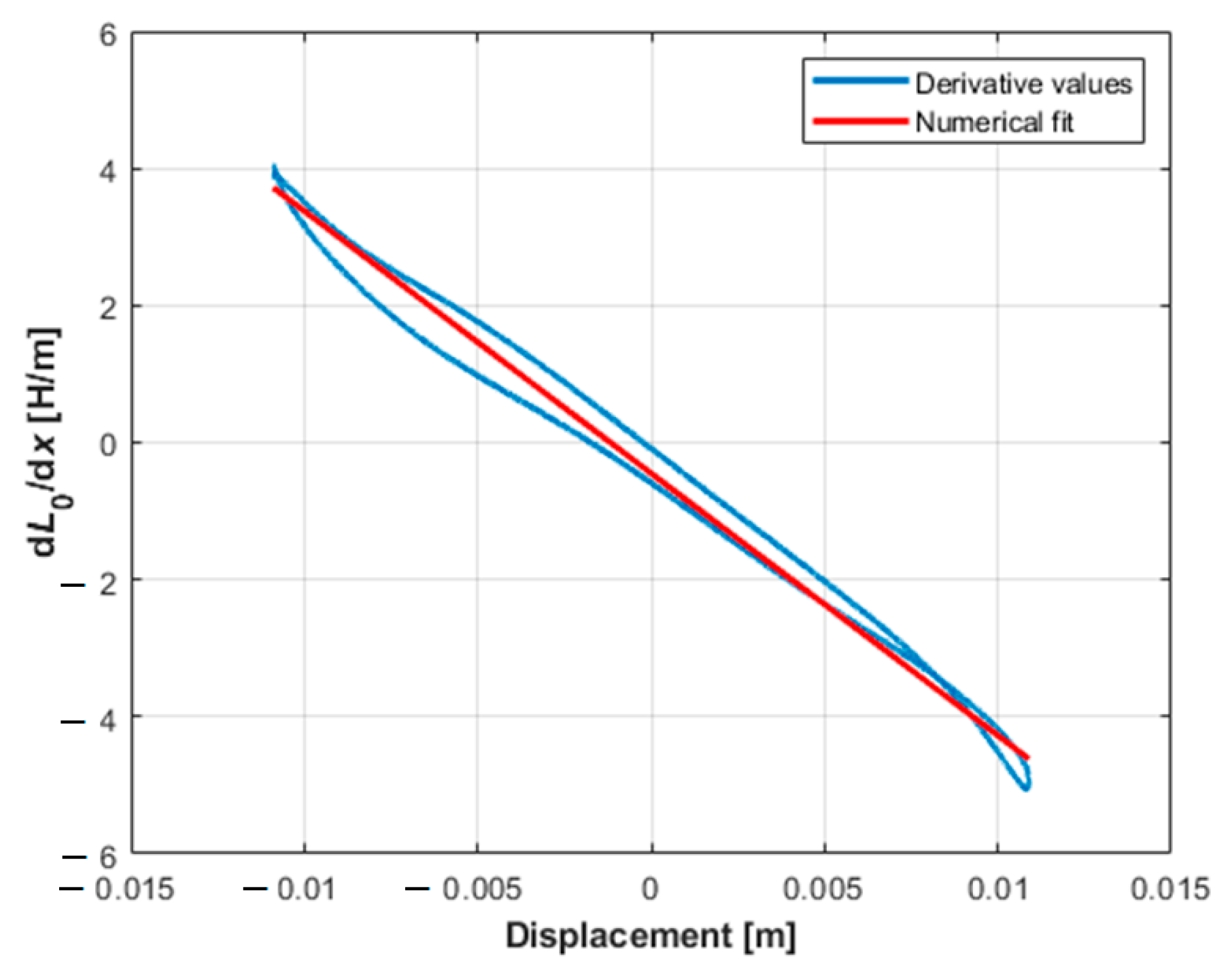
In both cases, the obtained values are fitted with a first-order polynomial according to the relations (19). Using these results, it is possible to determine the value of the derivative of the mutual inductance between the coils, as reported in (27). The expected trend of the derivatives should not depend on the relative displacement between the plates, but due to the constructive and assembly tolerance, there is an unavoidable variable misalignment of the axes of the coils that causes the trend depicted in Figure 11 (blue line), fitted with a horizontal line (red line).
The discrepancy between the theoretical and the experimental trend has been attributed to the imperfect parallelism between the axes of the coils, whose arrangement is also variable due to the slight deformability of the coil support. This effect has been theoretically confirmed by means of a finite element model in which the axes of the coils have been defined as not parallel to each other. This result leads to the need for an accurate positioning of the coils on a sufficiently rigid support. Therefore, although in Figure 9 to Figure 11 the experimental results assume a different trend from the theoretical ones, the proposed approach can be considered reliable; in fact, as shown below, the simulations performed considering the numerical trend fit produce results close to the experimental ones.
The following coefficient values were identified (Table 2) for the test rig:
The variable trend of was attributed to the mechanical misalignments after a series of sensitivity tests were performed using FEM software. By shifting the axis of the bottom coils of 1 and 5 mm, with respect to the center of the isolator, the curves reported in Figure 12 were obtained. It can be noted that the depicted trends have a parabolic trend very similar to the experimental ones. The misalignment is a common problem in real applications, but, as demonstrated in the following paragraph, the error introduced in the model has negligible effects.
The electromechanical behavior of the insulator was tested by adjusting the supply voltages of the coils to obtain the desired current value. A comparison between the magnetic forces obtained with the proposed model and those obtained experimentally is reported below. The tests were performed with a current (i0) in the lower coil of 3A and a variable current (i3) in the upper coil and by imposing a relative harmonic motion with an amplitude of 10.5 mm at a frequency of 0.25 Hz. The comparison is reported as a function of both time (Figure 13) and displacement (Figure 14). Both diagrams show that the proposed model provides a force trend in good agreement with that obtained experimentally, with an approximation that is similar to that found in papers by other researchers [18,19].
6.5. Force Capability of the Electromagnetic Actuator
The calculation of magnetic force by the model is carried out using the solution procedure for the current (where the transient terms are neglected) and the electrical-parameter-estimation methods mentioned above. The obtained results demonstrate a good agreement between the magnetic force calculated from the experimental data and the model-based magnetic force. Therefore, the electromagnetic model obtained allows the possibility of predicting the magnetic force generated by the coil, which is a fundamental achievement for the development of an isolator control.
The possibility of analyzing the force capability of the isolator is given by the obtained electromagnetic model. By fixing the currents in the upper coil of the isolator and considering a variable current in the bottom coils, the maximum values of electromagnetic force for each position along the x-axis can be obtained. These values are shown in the isovalues maps in Figure 15, Figure 16 and Figure 17.
According to the values of the upper coil current, it is possible to reach a force value of about 200 N. However, the most interesting point is the possibility of changing the force value for each position by varying the bottom coil currents. The same considerations can be carried out by considering a fixed current value for the bottom coils and varying the currents in the upper coil. As highlighted in Figure 18, for each value of the relative displacement, it is possible to vary the electromagnetic force according to the variation in the currents in the coils. These results are very important for the real-time control of the system, where the fast dynamic of the electromagnetic system can be exploited to change the isolator’s restoring force.
The experimental results show that the adopted electromagnetic topology has a higher number of tunable parameters with respect to those equipped with permanent magnets [18,19]; furthermore, electromagnetic systems are characterized by a high robustness and efficiency [22].
6.6. Trasmissibility
The theoretical model, including the parameters identified through laboratory tests, allows us to define the transmissibility of the system, expressed as the ratio between the amplitude Xm of the displacement of the body and the amplitude Xb of the displacement of the base (ground):
Indicating the relative displacement of the mass with with respect to the base (Figure 19), the equation of motion of the isolated body is
where m is the mass of the body.
Equation (29) contains the reaction of the elastomeric pad, defined in (2); the rolling resistance of the BTUs, defined in (1); and the magnetic force defined in (17) and (18), which can be expressed as
Table 2 reports the coefficients in Equation (30).
By forcing the base with a harmonic motion of constant amplitude and variable frequency, it is possible to obtain the ratio defined in (29) as a function of the excitation frequency. This evaluation can be carried out by powering the three coils in different ways. Figure 20 reports several curves, each obtained by considering that the lower coils (C1 and C2) are powered in the same way and keeping the power supply of the coils constant. The blue curve was obtained without feeding the coils. By increasing the current intensity, the peak of the curves assumes a higher value and is reached for higher values of the forcing frequency as the magnetic force determines a stiffening effect of the insulation system.
If the intensity of the current is controlled with the aim of keeping the body at rest in its initial position by properly defining the maximum values of the power supply, the curves no longer show areas of amplification of the transmissibility. In this case, the magnetic force acts in contrast to the elastic force, making the isolation system less stiff. Figure 21 shows the transmissibility curves obtained with a PID control for several values of the maximum intensity current; by increasing it, the transmissibility curve assumes a descending trend. In this condition, the trend of the amplitude displacement xb is imposed on the base (with constant amplitude and increasing frequency) and the amplitude displacement xm of the isolated body, which does not show the time intervals during which the amplitude of the motion is amplified with respect to that of the base (Figure 22).
Compared to other controlled isolators, the proposed one allows higher relative displacements with transmissibility lower than one. By way of example, it should be noted that the isolator presented in [18] was tested for relative displacements of less than 1 mm, while the proposed one was tested for relative displacements of 20 mm.
7. Conclusions
In this paper, a hybrid isolator to be used for horizontal vibrations coming from the ground is proposed. The isolator consists of passive elastomeric pads and an electromagnetic actuator that acts, for short instants of time, when the passive system cannot guarantee the isolation requirements. Compared to existing isolation systems, the proposed hybrid insulator has characteristics comparable to active ones, but it requires a lower contribution of external energy. The system is also reliable, as it can work, with less efficiency, even in the absence of external energy. The theoretical model proposed for the definition of the restoring force has provided results that effectively approximated the experimental ones obtained from a purpose-built test rig. Our simulations have confirmed that the proposed isolator, equipped with a control system, allows low transmissibility to be obtained for each exciting frequency.
Author Contributions
Conceptualization, L.P.D.N. and R.B.; methodology, L.P.D.N., R.B., G.D.M. and S.P.; software, L.P.D.N. and R.B.; validation, L.P.D.N., R.B., G.D.M. and S.P.; formal analysis, L.P.D.N., R.B., G.D.M. and S.P.; investigation, L.P.D.N. and G.D.M.; data curation, L.P.D.N. and G.D.M.; writing—original draft preparation, L.P.D.N. and S.P.; writing—review and editing, R.B. and S.P.; supervision, L.P.D.N., R.B., G.D.M. and S.P. All authors have read and agreed to the published version of the manuscript.
Funding
This research received no external funding.
Institutional Review Board Statement
Not applicable.
Informed Consent Statement
Not applicable.
Data Availability Statement
Not applicable.
Acknowledgments
The authors are grateful to Gennaro Stingo and Rosario Moreschi for their collaboration during the setup construction and the execution of laboratory tests.
Conflicts of Interest
The authors declare no conflict of interest.
Appendix A
Appendix B
References
Pradhan, P.; Singh, D. Review on air suspension system. Mater. Today Proc.2023, 81, 486–488. [Google Scholar] [CrossRef]
Eskandary, P.K.; Khajepour, A.; Wong, A.; Ansari, M. Analysis and optimization of air suspension system with independent height and stiffness tuning. Int. J. Automot. Technol.2016, 17, 807–816. [Google Scholar] [CrossRef]
Demetriades, G.; Constantinou, M.; Reinhorn, A. Study of wire rope systems for seismic protection of equipment in buildings. Eng. Struct.1993, 15, 321–334. [Google Scholar] [CrossRef]
Ni, Y.; Ko, J.; Wong, C. Identification of Non-Linear hysteretic isolators from periodic vibration tests. J. Sound Vib.1998, 217, 737–756. [Google Scholar] [CrossRef]
Pagano, S.; Strano, S. Wire rope springs for passive vibration control of a light steel structure. WSEAS Trans. Appl. Theor. Mech.2013, 3, 212–221. [Google Scholar]
Molyneux, W.G. The support of an aircraft for ground resonance tests: A survey of available methods. Aircr. Eng. Aerosp. Technol.1958, 30, 160–166. [Google Scholar] [CrossRef]
Huan, L.; Yancheng, L.; Jianchun, L. Negative stiffness devices for vibration isolation applications: A review. Adv. Struct. Eng.2020, 23, 1739–1755. [Google Scholar]
Eskandary-Malayery, F.; Ilanko, S.; Mace, B.; Mochida, Y.; Pellicano, F. Experimental and numerical investigation of a vertical vibration isolator for seismic applications. Nonlinear Dyn.2022, 109, 303–322. [Google Scholar] [CrossRef]
Zou, W.; Cheng, C.; Ma, R.; Hu, Y.; Wang, W. Performance analysis of a quasi-zero stiffness vibration isolation system with scissor-like structures. Arch. Appl. Mech.2020, 91, 117–133. [Google Scholar] [CrossRef]
Carrella, A.; Brennan, M.J.; Waters, T.P.; Lopes, V., Jr. Force and displacement transmissibility of a nonlinear isolator with high-static-low-dynamic-stiffness. Int. J. Mech. Sci.2012, 55, 22–29. [Google Scholar] [CrossRef]
Brancati, R.; Di Massa, G.; Pagano, S. Investigation on the Mechanical Properties of MRE Compounds. Machines2019, 7, 36. [Google Scholar] [CrossRef]
Brancati, R.; Di Massa, G.; Pagano, S.; Petrillo, A.; Santini, S. A combined neural network and model predictive control approach for ball transfer unit–magnetorheological elastomer–based vibration isolation of lightweight structures. J. Vib. Control.2020, 26, 1668–1682. [Google Scholar] [CrossRef]
Komatsuzaki, T.; Inoue, T.; Terashima, O. Broadband vibration control of a structure by using a magnetorheological elasto-mer-based tuned dynamic absorber. Mechatronics2016, 40, 128–136. [Google Scholar] [CrossRef]
Cao, L.; Downey, A.; Laflamme, S.; Taylor, D.; Ricles, J. Variable friction device for structural control based on duo-servo vehicle brake: Modeling and experimental validation. J. Sound Vib.2015, 348, 41–56. [Google Scholar] [CrossRef]
Mikułowski, G. Vibration isolation concept by switchable stiffness on a semi-active pneumatic actuator. Smart Mater. Struct.2021, 30, 075019. [Google Scholar] [CrossRef]
Zhang, F.; Shao, S.; Tian, Z.; Xu, M.; Xie, S. Active-passive hybrid vibration isolation with magnetic negative stiffness isolator based on Maxwell normal stress. Mech. Syst. Signal Process.2019, 123, 244–263. [Google Scholar] [CrossRef]
Sun, Y.; Meng, K.; Yuan, S.; Zhao, J.; Xie, R.; Yang, Y.; Luo, J.; Peng, Y.; Xie, S.; Pu, H. Modeling Electromagnetic Force and Axial-Stiffness for an Electromagnetic Negative-Stiffness Spring Toward Vibration Isolation. IEEE Trans. Magn.2019, 55, 3. [Google Scholar] [CrossRef]
Pu, H.; Yuan, S.; Peng, Y.; Meng, K.; Zhao, J.; Xie, R.; Huang, Y.; Sun, Y.; Yang, Y.; Xie, S.; et al. Multi-layer electromagnetic spring with tunable negative stiffness for semi-active vibration isolation. Mech. Syst. Signal Process.2019, 121, 942–960. [Google Scholar] [CrossRef]
Pham, M.-N.; Ahn, H.-J. A horizontal vibration isolator with electromagnetic planar actuator using multi hall-effect sensor network. In Proceedings of the 2013 International Conference on ICT Convergence (ICTC), Jeju, Republic of Korea, 14–16 October 2013; pp. 1093–1094. [Google Scholar] [CrossRef]
Hong, D.-K.; Park, J.-H. Electromagnetic Design and Analysis of Inertial Mass Linear Actuator for Active Vibration Isolation System. Actuators2023, 12, 295. [Google Scholar] [CrossRef]
Török, A.; Petrescu, S.; Feidt, M. Development in periodic series, method for resolving differential equations. arXiv2020, arXiv:2007.02554. [Google Scholar] [CrossRef]
Graham Kelly, S. Mechanical Vibrations. In Theory Appl. Cengage Learn.; 2012; ISBN 1439062129, 9781439062128. [Google Scholar]
Figure 1.
Molyneux spring device: (a) scheme; (b) force-displacement trend.
Figure 1.
Molyneux spring device: (a) scheme; (b) force-displacement trend.
Figure 2.
Vibration isolator scheme.
Figure 2.
Vibration isolator scheme.
Figure 3.
Three-dimensional scheme of the isolator lower plate.
Figure 3.
Three-dimensional scheme of the isolator lower plate.
Figure 4.
Reference system.
Figure 4.
Reference system.
Figure 5.
Scheme of the test rig.
Figure 5.
Scheme of the test rig.
Figure 6.
Photos of the test rig: overall view and components of the isolator.
Figure 6.
Photos of the test rig: overall view and components of the isolator.
Figure 9.
Values of (blue line) and the numerical fit (red line) with a current of 3A in the lower coils.
Figure 9.
Values of (blue line) and the numerical fit (red line) with a current of 3A in the lower coils.
Figure 10.
Values of (blue line) and the numerical fit (red line) with a current of 3 A in the upper coil.
Figure 10.
Values of (blue line) and the numerical fit (red line) with a current of 3 A in the upper coil.
Figure 11.
Values of (blue line) and the numerical fit (red line) with a current of 3A in the coils.
Figure 11.
Values of (blue line) and the numerical fit (red line) with a current of 3A in the coils.
Figure 12.
Values of obtained with a misalignment of 1 mm (grey lines) and 5 mm (black lines) of the axis of the bottom coils, with a current of 3 A in the coils.
Figure 12.
Values of obtained with a misalignment of 1 mm (grey lines) and 5 mm (black lines) of the axis of the bottom coils, with a current of 3 A in the coils.
Figure 13.
Measured magnetic force (blue) and model magnetic force (red) vs. time.
Figure 13.
Measured magnetic force (blue) and model magnetic force (red) vs. time.
Figure 14.
Measured magnetic force (blue) and model magnetic force (red) vs. displacement.
Figure 14.
Measured magnetic force (blue) and model magnetic force (red) vs. displacement.
Figure 15.
Force isovalues (N) map for the upper coil current of 1 A and the bottom coils’ currents in the range from −3 A to 3 A.
Figure 15.
Force isovalues (N) map for the upper coil current of 1 A and the bottom coils’ currents in the range from −3 A to 3 A.
Figure 16.
Force isovalues (N) map for the upper coil current of 3 A and the bottom coils’ currents in the range from −3 A to 3 A.
Figure 16.
Force isovalues (N) map for the upper coil current of 3 A and the bottom coils’ currents in the range from −3 A to 3 A.
Figure 17.
Force isovalues (N) map for the upper coil current of 5 A and the bottom coils’ currents in the range −3 A to 3 A.
Figure 17.
Force isovalues (N) map for the upper coil current of 5 A and the bottom coils’ currents in the range −3 A to 3 A.
Figure 18.
Force value for the bottom coil current of 3 A and the upper coil’s current in the range from −5 A to 5 A.
Figure 18.
Force value for the bottom coil current of 3 A and the upper coil’s current in the range from −5 A to 5 A.
Figure 19.
Dynamic scheme.
Figure 19.
Dynamic scheme.
Figure 20.
Transmissibility with a constant current feeding the coils.
Figure 20.
Transmissibility with a constant current feeding the coils.
Figure 21.
Transmissibility with controlled current feeding the coils.
Figure 21.
Transmissibility with controlled current feeding the coils.
Figure 22.
Comparison between the motion imposed on the base and the motion of the mass.
Figure 22.
Comparison between the motion imposed on the base and the motion of the mass.
Table 1.
Coil characteristics.
Table 1.
Coil characteristics.
Characteristic
Dimension
Coil external diameter
0.130 m
Coil ferromagnetic core height
0.044 m
Coil windings height
0.030
Number of turns
1000
Air gap
0.003 m
Distance between the centers of the lower coils
0.150 m
Coil electrical resistance
10.6 Ω
Copper wire diameter
AWG 20
Table 2.
Values of the coefficients obtained with the fitting of the trend of the derivatives.
Table 2.
Values of the coefficients obtained with the fitting of the trend of the derivatives.
−382 H/m2
−0.449 H/m
−333 H/m2
−0.757 H/m
−9.35 H/m
Disclaimer/Publisher’s Note: The statements, opinions and data contained in all publications are solely those of the individual author(s) and contributor(s) and not of MDPI and/or the editor(s). MDPI and/or the editor(s) disclaim responsibility for any injury to people or property resulting from any ideas, methods, instructions or products referred to in the content.
Brancati, R.; Di Massa, G.; Di Noia, L.P.; Pagano, S.
A Hybrid Vibration Isolator Based on Elastomeric and Electromagnetic Restoring Force. Appl. Sci.2023, 13, 9594.
https://doi.org/10.3390/app13179594
AMA Style
Brancati R, Di Massa G, Di Noia LP, Pagano S.
A Hybrid Vibration Isolator Based on Elastomeric and Electromagnetic Restoring Force. Applied Sciences. 2023; 13(17):9594.
https://doi.org/10.3390/app13179594
Chicago/Turabian Style
Brancati, Renato, Giandomenico Di Massa, Luigi Pio Di Noia, and Stefano Pagano.
2023. "A Hybrid Vibration Isolator Based on Elastomeric and Electromagnetic Restoring Force" Applied Sciences 13, no. 17: 9594.
https://doi.org/10.3390/app13179594
APA Style
Brancati, R., Di Massa, G., Di Noia, L. P., & Pagano, S.
(2023). A Hybrid Vibration Isolator Based on Elastomeric and Electromagnetic Restoring Force. Applied Sciences, 13(17), 9594.
https://doi.org/10.3390/app13179594
Note that from the first issue of 2016, this journal uses article numbers instead of page numbers. See further details here.
Article Metrics
No
No
Article Access Statistics
For more information on the journal statistics, click here.
Multiple requests from the same IP address are counted as one view.
Brancati, R.; Di Massa, G.; Di Noia, L.P.; Pagano, S.
A Hybrid Vibration Isolator Based on Elastomeric and Electromagnetic Restoring Force. Appl. Sci.2023, 13, 9594.
https://doi.org/10.3390/app13179594
AMA Style
Brancati R, Di Massa G, Di Noia LP, Pagano S.
A Hybrid Vibration Isolator Based on Elastomeric and Electromagnetic Restoring Force. Applied Sciences. 2023; 13(17):9594.
https://doi.org/10.3390/app13179594
Chicago/Turabian Style
Brancati, Renato, Giandomenico Di Massa, Luigi Pio Di Noia, and Stefano Pagano.
2023. "A Hybrid Vibration Isolator Based on Elastomeric and Electromagnetic Restoring Force" Applied Sciences 13, no. 17: 9594.
https://doi.org/10.3390/app13179594
APA Style
Brancati, R., Di Massa, G., Di Noia, L. P., & Pagano, S.
(2023). A Hybrid Vibration Isolator Based on Elastomeric and Electromagnetic Restoring Force. Applied Sciences, 13(17), 9594.
https://doi.org/10.3390/app13179594
Note that from the first issue of 2016, this journal uses article numbers instead of page numbers. See further details here.


