Distributional Representation of Cyclic Alternating Patterns for A-Phase Classification in Sleep EEG

Abstract

This article describes a detailed methodology for the A-phase classification of the cyclic alternating patterns (CAPs) present in sleep electroencephalography (EEG). CAPs are a valuable EEG marker of sleep instability and represent an important pattern with which to analyze additional characteristics of sleep processes, and A-phase manifestations have been linked to some specific conditions. CAP phase detection and classification are not commonly carried out routinely due to the time and attention this problem requires (and if present, CAP labels are user-dependent, visually evaluated, and hand-made); thus, an automatic tool to solve the CAP classification problem is presented. The classification experiments were carried out using a distributional representation of the EEG data obtained from the CAP Sleep Database. For this purpose, data symbolization was performed using the one-dimensional symbolic aggregate approximation (1d-SAX), followed by the vectorization of symbolic data with a trained Doc2Vec model and a final classification with ten classic machine learning models for two separate validation strategies. The best results were obtained using a support vector classifier with a radial basis kernel. For hold-out validation, the best F1 Score was 0.7651; for stratified 10-fold cross-validation, the best F1 Score was 0.7611 ± 0.0133. This illustrates that the proposed methodology is suitable for CAP classification.

1. Introduction

Sleep is a reversible behavioral state characterized by unresponsiveness and perceptual disengagement from the environment [1]. Sleep is studied systematically through polysomnography (PSG), in which electroencephalography (EEG), electrooculography (EOG), electromyography (EMG), electrocardiography (ECG), and respiratory signals (such as pulse oximetry, airflow, and respiratory effort) are recorded to help experts understand the physiological sleep processes and evaluate the underlying causes of diverse sleep disturbances.

The EEG signals extracted from PSG, also named sleep EEG, contain valuable information about the structure of sleep that is organized and analyzed through its macro and micro-structure.

The so-called sleep macro-structure is defined as the basic structural organization of normal sleep, which is presented in cycles and is classified into two main types.

• Rapid eye-movement (REM) sleep: This is also named active sleep after the presence of rapid eye movements and the possibility of having dreams.
• Non-rapid eye-movement (NREM) sleep: This is also named inactive sleep and is subdivided into the stages N1, N2, and N3, each meaning a more profound (i.e., less responsive to the environment) sleep state.

On the other hand, sleep micro-structure is defined by the quantification of the graphic elements present in the different sleep stages. The list of these graphic elements includes sleep spindles, slow-wave activities, sharp waves, arousals, and cyclic alternating patterns [2]. It is important to state that the mentioned graphic elements are usually short-length and user-dependent, and, if present, their labels are visually evaluated and hand-made by sleep experts, which may lead to human mistakes.

Further to being inherently time- and effort-consuming, sleep descriptors are typically evaluated using vastly different signal processing (or visual) techniques. This makes it more challenging to combine the findings into a consistent description of the sleep processes at both the macro and micro levels.

1.1. Cyclic Alternating Pattern

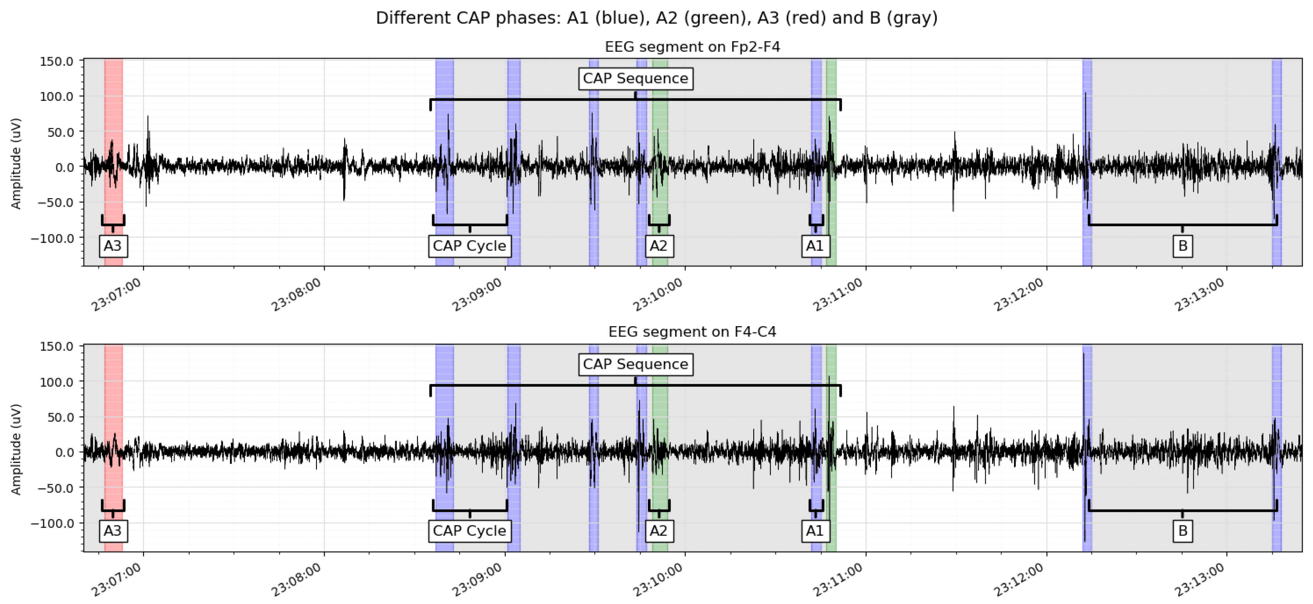
The object of this study is the cyclic alternating pattern (CAP), defined by an alternating sequence of two characteristic EEG patterns, each lasting between 2 and 60 seconds [3]. These patterns are the A-phase, which is composed of lumps of sleep phasic events, and the B-phase, which is simply the return to the background EEG.

The sequence of A-B phases is also called a CAP cycle. Yet, there is another sequence composed of the same EEG patterns. This is the CAP sequence, which contains at least two complete CAP cycles in succession. The minimum content of a CAP sequence is, therefore, A-B-A-B. Examples of CAP cycles and sequences are shown in Figure 1.

Furthermore, A-phase activities are classified referring to the proportion of EEG synchrony (high-voltage slow waves) and EEG desynchrony (low-voltage fast rhythms) presented throughout the A-phase. The three A-phase types are:

• A1: EEG activity is dominated by EEG synchrony and, if present, EEG desynchrony occupies less than 20% of the complete A-phase duration;
• A2: EEG activity is a combination of slow and fast rhythms, with EEG desynchrony occupying between 20% and 50% of the entire A-phase;
• A3: Fast, low-amplitude rhythms dominate EEG activity, and strictly more than 50% of the A-phase is occupied by EEG desynchrony.

Terzano et al. (2001) [4] described the detailed rules to score the CAP since it is considered a valuable EEG marker of unstable sleep. CAP rate is an interesting CAP-related parameter that can be computed by following these rules.

The CAP rate measures the brain’s effort to maintain sleep [5] and is proven to increase under conditions that cause vigilance instability, including noise [6], insomnia [7], periodic leg movements [8], nocturnal seizures [9], and certain severe diseases such as s-stage coma [10], and Creutzfeldt–Jakob disease (CJD) [11].

In the same direction, manifestations of CAP phases have been linked to some specific phenomena. For example, the A-phase represents a favorable condition for the onset of nocturnal motor seizures in generalized and local (frontotemporal) epilepsy [9], bruxism [12], and periodic leg movements [13].

On the other hand, the B-phase appears to be chronologically related to inhibitory events in nocturnal myoclonus in epileptic patients [5,9].

Additionally, CAP is a valuable parameter in the research of sleep disorders across all live stages since it can be detected both in child and adult sleep [14]. Thus, the detection and classification of CAPs are meaningful to understanding some physiological and pathological sleep processes.

However, CAP detection and classification are commonly not carried out routinely due to the time and attention this problem requires. An automatic tool to solve this task would be helpful to massively analyze CAPs and possibly unravel new interesting relations between CAPs and different health conditions.

1.2. Hypothesis

Even though there are numerous investigations on the automatic detection and classification of a CAP and its sub-types (as discussed in Section 2), this research focuses on the implementation of natural language processing (NLP) and pattern recognition techniques on the same problem.

The main reason for exploring these techniques is to (i) reduce the complexity of the problem by representing the time-series data as shorter sequences of symbols and (ii) try to obtain interpretable results by applying NLP techniques such as word embeddings.

Word embeddings are a vectorial representation of words for text analysis, as proposed in [15]. This representation is based on mapping words (included in a collection of phrases or documents) to real-number vectors that rely on the distributional hypothesis. This hypothesis was popularized by Joseph R. Firth in 1957, who stated that “words that occur in similar contexts tend to have similar meanings” [16].

By assuming that signals can be translated into symbols and then organized as “words”, they can also be, theoretically, represented as word embeddings. Then, the embeddings can be analyzed with machine learning models, as carried out in NLP.

This being the case, the hypothesis for this research is that using a distributional approach (based on the distributional hypothesis) for EEG signal representation will allow for the implementation of NLP techniques to solve the CAP detection and classification problem. This will be achieved using a context-based vectorial representation of signal segments as if they were words or phrases in a text.

2. Literature Review

This section reviews some of the most relevant investigations for this research and is divided into two subsections. Section 2.1 will describe some recent research works on time-series data mining and sleep macro-structure analysis. Section 2.2 will review some research works on micro-structure analysis, specifically on CAP detection and classification.

2.1. Time Series Data Mining

Data mining (DM) is a set of methodologies that analyze large datasets, aiming to identify patterns and relationships that can help solve different types of problems. This is achieved by four main processes: data gathering, data preparation, data mining/processing, and a final analysis and interpretation of the results [17]. Time-series data mining (TSDM) applies these processes to sequential data, i.e., data recorded over time [18].

However, when analyzing some specific time series (such as biomedical signals), TSDM focuses on particular areas of interest, known as events, instead of evaluating the entire time series [19]. Hence, this subsection describes some of the research works on TSDM that are interesting for the present proposal.

Li et al. (2012) developed a methodology to visualize variable-length time-series motifs by implementing the symbolic aggregate approximation (SAX) [20]. A grammar-based compression algorithm (greedy and heuristic) was implemented for motif detection. This methodology was performed on ECG signals, and the results demonstrated that recurrent patterns can be effectively identified with grammar induction in time series, even without prior knowledge of their lengths.

Wave2Vec is a tool for vectorizing EEG signals to predict a brain disease (alcoholic vs. non-alcoholic patients) proposed by Kim et al. (2018) [21]. This prediction was achieved by quantizing fixed-length EEG segments to one of the hexadecimal symbols of a fixed “bag-of-symbols”. Subsequently, vectorization was performed with a similar model to Word2Vec. Finally, three classification models based on deep neural networks (DNN), convolutional neural networks (CNN), and recurrent neural networks (RNN) were compared.

Grammar induction for detecting anomalies in time series was implemented by Gao et al. in 2020 [22]. This research was carried out on ECG signals transformed into symbols with SAX. The resulting symbolic sequences were analyzed through another NLP technique named grammar induction, where a set of rules that best describes the analyzed phenomena is found. Numerosity reduction was performed to simplify the rules found by the algorithm and to finally implement a “Rule Density Function” for anomaly detection.

It is essential to mention that the previous research had objectives substantially different from those of the current research. Li et al. (2012) [20] and Gao et al. (2020) [22] used ECG signals, which are significantly more periodic than EEG. Although Kim et al. (2018) [21] implemented their tool on EEG signals, they were searching for another type of information within them (to predict alcoholism). None of the previous examples use sleep EEG or search for CAPs.

In recent years, sleep analysis, especially the sleep staging task, has also been explored [23,24]. Nevertheless, the methodologies proposed to solve this task are only indirectly related to the current research, which inquires into the symbolic transformation and/or vectorization of the signals.

Sleep stage classification labels 30-second-long PSG segments, known as sleep epochs. The labels are usually visually scored and divided into deep-sleep, light-sleep, and awake or, more precisely, S1 or N1, S2 or N2, S3 or N3, and R or REM, which are used to analyze sleep macro-structure.

In this direction, Joe et al. (2022) [23] analyzed EEG and EOG images in terms of their time and frequency domains by using a CNN on the Sleep-EDFx dataset [25]. They achieved results of 94% both in accuracy and F1 scores. Alternatively, Zhang et al. (2023) [24] analyzed a single channel (ECG) to analyze the sleep structure of three different datasets, obtaining accuracy values of 0.849, 0.827, and 0.868.

2.2. CAP Detection and Classification

For sleep micro-structure analysis, Rosa et al. (1999) pioneered the automatic detection of CAP sequences during sleep. They implemented feature extraction and detection with the maximum likelihood and a variable length template-matched filter [26]. The preliminary results of classifying CAP vs. Non-CAP segments were achieved by using a state machine ruled-based decision system on a group of four middle-aged adults.

A tool to analyze the micro and macro-structure of sleep EEG was implemented by Malinowska et al. (2006) [27]. They detected deep-sleep stages and arousals, the continuous description of slow wave sleep, and the measure of spindling activity by using adaptive time-frequency approximations with the matching pursuit (MP) algorithm. Though quantifiable results were not reported in this research, this tool is relevant due to the interest in automating sleep EEG analysis since 2006.

More recently, Hartmann et al. (2019) [28] implemented a long short-term memory (LSTM) model to detect A-phases and classify them into three subtypes: A1, A2, and A3. From the CAP Sleep Database, they removed epochs marked as “Awake” and “REM Sleep” and worked with two patient subsets: 16 healthy patients and 30 diagnosed with nocturnal frontal-lobe epilepsy (NFLE). They achieved averaged F1 scores ranging from 57.37% to 67.66% in the different modalities of classification (A-phase vs. non-A-phase and A1 vs. A2 vs. A3 vs. B), as shown in

Table 1. Literature review regarding CAP detection and classification.

Author (Year)	Methodology	Dataset (Data Subset)	Classification	Metrics
Hartmann et al. (2019) [28]	Resampling (128 Hz), removing Wake and REM epochs, filtering, and feature extraction for an LSTM, with LOO Cross-Validation.	CAP Sleep Database (n = 46: 16 Healthy, 30 Pathological-NFLE)	A-phase vs. Non-A-phase	F1 Score, Recall, Precision, Accuracy, Specificity
			A-phases (A1 vs. A2 vs. A3) vs. B-phase	F1 Score, Precision and Recall per class, Accuracy
Arce Santana et al. (2020) [29]	Segmentation (4 s), spectrogram computation. Image classification with a deep 2D-CNN model.	CAP Sleep Database (n = 9: Healthy)	A-phase vs. Non-A-phase	Average Accuracy
			A-phases (A1 vs. A2 vs. A3)	Average Accuracy
Loh et al. (2021) [30]	Segmentation (2 s), standardization, classification (1D-CNN Model) for sleep stages and CAP patterns.	CAP Sleep Database (n = 6: Healthy) - Balanced	A-phase vs. B-phase	F1 Score, Recall, Precision, Accuracy, Specificity
		CAP Sleep Database (n = 6: Healthy) - Unbalanced	A-phase vs. B-phase	F1 Score, Recall, Precision, Accuracy, Specificity
Tramonti Fantozzi et al. (2021) [31]	Segmentation (90 s, shifts of 30 s), band-pass filtering, threshold, adapted Ferri’s algorithm with Local analysis (channel F4-C4).	CAP Sleep Database (n = 41: 8 Healthy, 33 Pathological-Diverse)	A-phase vs. Non-A-phase	F1 Score, Recall, Precision, False discovery rate (FDR) and False negative rate (FNR)
	Segmentation (90 s, shifts of 30 s), band-pass filtering, threshold, adapted Ferri’s algorithm with Local Multi-trace analysis.	CAP Sleep Database (n = 41: 8 Healthy, 33 Pathological-Diverse)	A-phase vs. Non-A-phase	F1 Score, Recall, Precision, False discovery rate (FDR) and False negative rate (FNR)
You et al. (2022) [32]	Resampling (128 Hz), removing Wake and REM epochs, for a Gated Transformer-based U-Net framework with a curriculum-learning strategy.	CAP Sleep Database (n = 46: 16 Healthy, 30 Pathological-NFLE)	A-phase vs. Non-A-phase	F1 Score, Recall, Precision, Accuracy, Specificity, Area under the ROC Curve (AUC)
			A-phases (A1 vs. A2 vs. A3) vs. B-phase	F1 Score and Recall per class, Accuracy
	Resampling (128 Hz) for a Gated Transformer-based U-Net framework with a curriculum-learning strategy.	CAP Sleep Database (n = 46: 16 Healthy, 30 Pathological-NFLE)	A-phase vs. Non-A-phase	F1 Score, Recall, Precision, Accuracy, Specificity, Area under the ROC Curve (AUC)
			A-phases (A1 vs. A2 vs. A3) vs. B-phase	F1 Score and Recall per class, Accuracy

n = number of PSG recordings considered.

.

A two-dimensional convolutional neural network (2D-CNN) was implemented by Arce Santana et al. (2020) [29] to detect A-phases and classify them into the A1, A2, and A3 subtypes by using a different approach. They segmented nine EEG recordings in 4-second long epochs and computed their spectrograms, which are visual representations of the frequency content of a time series. They fed the resulting images to a deep 2D-CNN and obtained mean accuracy scores of 88.09% in A-phase detection and 77.31% in A-phase classification (A1 vs. A2 vs. A3). Unfortunately, no other metric is reported, restricting the performance analysis within unbalanced data, which is the case of the A-phase subtypes.

The automated detection of CAPs and the classification of sleep stages using a deep neural network was proposed by Loh et al. (2021) [30]. Six healthy patients from the CAP Sleep Database were used to segment, standardize, and classify the sleep stages and CAP patterns with a one-dimensional convolutional neural network model (1D-CNN). Loh et al. (2021) reported F1 scores of 75.34% and 33.04% for CAP detection in a balanced and an unbalanced dataset, respectively. Overall, the summarized metrics shown in Table 1 reveal that the model performs better on the balanced dataset than on the unbalanced dataset. This is directly caused by the number of B-phase examples (87.4% of the unbalanced dataset), which increased the difficulty of identifying the A-phase examples.

A novel approach was explored by Tramonti Fantozzi et al. (2021) to automate A-phase detection (A-phase vs. Non-A-phase) through local and multi-trace analysis [31]. They found that channel F4-C4 performed better than all the other analyzed channels, achieving F1 scores from 61.38% to 63.88% via local analysis on this channel. In comparison, their multi-trace approach resulted in F1 scores ranging from 64.34% to 66.78% on the different patient subsets. A total of 41 recordings from the CAP Sleep Database were analyzed in this research. Further details of the data and the methodology are shown in Table 1.

Finally, the GTransU-CAP model was designed by You et al. (2022) [32], and this was trained on the same data subset from [28]. This model represents an automatic labeling tool for CAPs in sleep EEG, using a gated transformer-based U-Net framework with a curriculum-learning strategy. In A-phase detection, F1 scores of 67.78% in healthy patients and 72.16% in patients with nocturnal front lobe epilepsy (NFLE) were achieved. For the A-phase subtype classification, the non-weighted average F1 scores are 59.45% and 59.55% for healthy and epileptic patients, respectively.

A summary of the previous literature review is presented in Table 1, where the different methodologies and classification approaches can be identified. Additionally, a list of the metrics reported for each approach is included in the last column. The diversity of the used data subsets, classification approaches, and performance measurements reported by the researchers hinders a direct comparison between them.

As described in Table 1, a diverse range of A-phase classification methodologies exist, and a key point stood out: only three investigations included the identification of A-phase subtypes (A1, A2, and A3) under two different classification strategies (one including only A-phase subtypes and the second including also B-phases). Thus, there is still a window of opportunity to solve the A-phase classification problem.

The literature review’s extended results are presented in

Table A1. Extended results of the literature review and a comparison with the current research results.

Author (Year)	Classification	Accuracy (%)	F1 Score (%)	Recall (%)	Precision (%)
Hartmann et al. (2019) [28]	A vs. Non-A	86.43 ± 4.62 (n = 16) 85.09 ± 4.54 (n = 30)	63.46 ± 8.22 (n = 16) 67.66 ± 7.03 (n = 30)	76.10 ± 14.47 (n = 16) 78.48 ± 8.66 (n = 30)	54.42 ± n/a (n = 16) 59.46 ± n/a (n = 30)
	A1 vs. A2 vs. A3 vs. B	81.89 ± 6.84 (n = 16) 78.27 ± 4.95 (n = 30)	57.53 (n = 16) * 57.37 (n = 30) *	65.39 (n = 16) * 65.37 (n = 30) *	52.90 (n = 16) * 53.62 (n = 30) *
Arce Santana et al. (2020) [29]	A vs. Non-A	88.09 (n = 9)	-	-	-
	A1 vs. A2 vs. A3	77.31 (n = 9)	-	-	-
Loh et al. (2021) [30]	A vs. B: balanced data	73.64 (n = 6)	75.34 (n = 6)	80.29 (n = 6)	70.96 (n = 6)
	A vs. B: unbalanced data	52.99 (n = 6)	33.04 (n = 6)	92.06 (n = 6)	20.13 (n = 6)
Tramonti Fantozzi et al. (2021) [31]	A vs. Non-A: Local Analysis	- - -	63.39 ± 9.10 (n = 41) 61.38 ± 8.33 (n = 8) 63.88 ± 9.34 (n = 33)	71.13 ± 12.53 (n = 41) 75.23 ± 10.59 (n = 8) 70.14 ± 12.91 (n = 33)	59.89 ± 13.97 (n = 41) 52.32 ± 8.38 (n = 8) 61.73 ± 14.52 (n = 33)
	A vs. Non-A: Multi-trace Analysis	- - -	66.31 ± 8.08 (n = 41) 64.34 ± 5.81 (n = 8) 66.78 ± 8.54 (n = 33)	82.68 ± 9.15 (n = 41) 87.41 ± 7.04 (n = 8) 81.54 ± 9.32 (n = 33)	57.12 ± 12.66 (n = 41) 51.29 ± 6.69 (n = 8) 58.53 ± 13.42 (n = 33)
You et al. (2022): only NREM [32]	A vs. Non-A	92.52 ± 1.39 (n = 16) 90.86 ± 2.00 (n = 30)	62.41 ± 9.34 (n = 16) 68.22 ± 6.33 (n = 30)	63.59 ± 15.64 (n = 16) 70.02 ± 10.42 (n = 30)	64.45 ± 10.72 (n = 16) 68.46 ± 10.35 (n = 30)
	A1 vs. A2 vs. A3 vs. B	88.11 ± 2.12 (n = 16) 85.61 ± 2.78 (n = 30)	53.98 (n = 16) * 56.99 (n = 30) *	59.32 (n = 16) * 61.07 (n = 30) *	- -
You et al. (2022) [32]	A vs. Non-A	90.26 ± 2.88 (n = 16) 88.89 ± 1.83 (n = 30)	67.78 ± 8.67 (n = 16) 72.16 ± 5.81 (n = 30)	68.15 ± 12.70 (n = 16) 72.05 ± 10.69 (n = 30)	69.13 ± 9.16 (n = 16) 74.30 ± 9.52 (n = 30)
	A1 vs. A2 vs. A3 vs. B	85.39 ± 5.88 (n = 16) 81.21 ± 4.40 (n = 30)	59.45 (n = 16) * 59.55 (n = 30) *	61.75 (n = 16) * 63.36 (n = 30) *	- -
This work: D2V output dim = 50	A1 vs. A2 vs. A3: HOV	75.68 (n = 21)	76.32 (n = 21)	75.68 (n = 21)	77.13 (n = 21)
	A1 vs. A2 vs. A3: KFCV	75.33 ± 1.41 (n = 21)	76.11 ± 1.33 (n = 21)	75.33 ± 1.41 (n = 21)	77.18 ± 1.28 (n = 21)
This work: D2V output dim = 100	A1 vs. A2 vs. A3: HOV	75.90 (n = 21)	76.49 (n = 21)	75.90 (n = 21)	77.24 (n = 21)
	A1 vs. A2 vs. A3: KFCV	75.39 ± 1.64 (n = 21)	76.09 ± 1.57 (n = 21)	75.39 ± 1.65 (n = 21)	77.05 ± 1.51 (n = 21)
This work: D2V output dim = 300	A1 vs. A2 vs. A3: HOV	75.95 (n = 21)	76.51 (n = 21)	75.95 (n = 21)	77.20 (n = 21)
	A1 vs. A2 vs. A3: KFCV	75.16 ± 1.10 (n = 21)	75.91 ± 1.11 (n = 21)	75.16 ± 1.10 (n = 21)	76.95 ± 1.21 (n = 21)
This work: D2V output dim = 500	A1 vs. A2 vs. A3: HOV	74.69 (n = 21)	75.43 (n = 21)	74.69 (n = 21)	75.38 (n = 21)
	A1 vs. A2 vs. A3: KFCV	74.80 ± 1.74 (n = 21)	75.67 ± 1.71 (n = 21)	74.80 ± 1.74 (n = 21)	76.90 ± 1.75 (n = 21)

n: number of sleep EEG recordings considered, HOV: hold-out validation, KFCV: K-fold cross-validation. * Non-weighted average between the reported metrics for each class (B, A1, A2, and A3).

, which reveals that classifying the naturally unbalanced CAP data is not trivial. The number of B-phases compared to A-phases hinders A-phase detection [30]. Moreover, the nature of the A2 subtype (basically, a mixture of A1 and A3) hampers its correct classification [28,32].

Finally, since none of the previous works reviewed a symbolic or distributional approach to sleep micro-structure analysis, there is a chance to explore these approaches and implement new tools based on them.

3. Materials and Methods

In this section, the proposed methodology is described in four subsections. First, the selected database is described. Second, the process of symbolization of the EEG signals is detailed. Third, the vectorization tool is defined. Finally, the proposed classification models and the evaluation metrics are detailed.

Figure 2 shows the flowchart corresponding to the methodology implemented for ➀ dataset selection, ➁ symbolic transformation, and ➂ the vectorization process, including the Doc2Vec non-supervised training. The final step of the first part of the methodology is ➃ to save the concatenated vectorized data.

The classification steps are described in Figure 3, where the proposed architectures for classification under two different validation strategies are detailed. This methodology starts with ➄ concatenated vectorized data loading, followed by ➅ data splitting, and the ➆ model’s training and testing under the corresponding validation strategy. Finally, the ➇ evaluation metrics are computed for ➈ model comparisons or performance averaging.

These processes are shown in parallel for simplicity, although hold-out validation was implemented before the K-fold cross-validation in order to be able to exclusively select and analyze the best-performing model.

In contrast to the methodology described to train the Doc2Vec models (Figure 2), where unsupervised learning is implemented, supervised learning is used to train the classification models (Figure 3).

3.1. CAP Sleep Database

The CAP research team led by Terzano et al. (2001) [4] released in 2012 the CAP Sleep Database on PhysioNet [33]. It consists of 108 PSG recordings that were registered by the Sleep Disorders Center of the Maggiore Hospital in Parma, Italy.

From the 108 PSG, 16 correspond to the recordings of healthy patients, and 92 correspond to the pathological recordings of patients diagnosed with:

• Nocturnal Frontal Lobe Epilepsy (NFLE)—40 recordings;
• REM Behaviour Disorder (RBD)—22 recordings;
• Periodic Leg Movement (PLM)—10 recordings;
• Insomnia—9 recordings;
• Narcolepsy—5 recordings;
• Sleep-disordered breathing (SDB)—4 recordings;
• Bruxism—2 recordings.

These recordings include at least three EEG signals with complementary EOG, chin and tibial EMG, airflow, respiratory effort, pulse oximetry, and ECG signals. In addition, they include annotations of the sleep stage and CAP labels (CAP1, CAP2, and CAP3, corresponding to the three A-phase types).

Each recording has an average duration of 9 hours (a complete night of sleep) with different sample frequency values (from 50 to 512 Hz). The interesting annotations in this research, i.e., CAP1, CAP2, and CAP3, have an average total duration of 16 minutes. This accounts for approximately only 3% of the complete recording.

For the first approach to the problem, the second largest group of patients was selected, i.e., the 22 RBD recordings. Additionally, channels Fp2-F4, F4-C4, Fp1-F3, and F3-C3 were selected due to the presence of CAPs in the frontocentral regions of the brain [34]. Figure 4 schematizes the electrode placements for the selected channels (red and blue), following the 10–20 system [35].

An analysis of the selected data showed that the blue channels (Fp2-F4 and F4-C4) were present in 21 out of the 22 recordings, whereas the red and blue channels (Fp2-F4, F4-C4, Fp1-F3, and F3-C3) were present in only 16 out of the 22 recordings. This analysis determined the data for the experiments described in this document: 21 RBD recordings for channels Fp2-F4 and F4-C4 (Figure 2 ➀).

3.2. Data Symbolization

The first step for data symbolization was segmentation, which changed the total duration of the signals into N-second segments for each recording—Each recording has a different duration in hours, hence, a different N value. Once the 21 recordings were split into one-second segments, they were processed through one-dimensional symbolic aggregate approximation (1d-SAX); see Figure 2 ➁.

In order to better understand 1d-SAX symbolic transformation, it is necessary to understand symbolic aggregate approximation (SAX) and piecewise aggregate approximation (PAA):

• PAA is a time series downsampling in which the mean value of each fixed-sized segment is retained [36];
• SAX is based on PAA but performs an additional quantization of the mean value. Under the assumption that the time series follows a standard normal distribution, the quantization boundaries are computed to ensure that the symbols are assigned to each quantized mean value with equal probability [37];
• 1d-SAX is a symbolic representation of a time series based on SAX. This representation contains information about each segment’s slope and a symbol that is associated with the segment’s mean value. In other words, each segment is represented by an affine function of two quantized parameters: the slope and mean value [38].

In this particular case, the mean value is represented with 1 of the 26 letters in the lowercase English alphabet $a,b,c,\dots ,y,z$, whereas the slope is represented with an integer between 1 and 10. Hence, the number of 1d-SAX symbols created by combining a letter and an integer is 260. Examples of the final symbols are $a1,b8,c4,d3,e7,f2$, and so on, with all of these having a specific meaning of the segment’s features. The 1d-SAX symbols will be referred to as “words” from now on.

Thus, “phrases” will refer to the sequences of “words” corresponding to the symbolic one-second segments obtained from each channel—Each channel was analyzed separately. These unlabeled symbolic “phrases” were used to train the model described in Section 3.3 using unsupervised learning.

On the other hand, a structured database was created with longer “phrases” corresponding to the CAP labeled segments; for reference, the CAP A-phase duration is between 2 and 60 s. The classification experiments (see Section 3.4) were carried out using this structured database with supervised learning.

3.3. Data Vectorization

A well-known type of word representation is word embeddings, which can capture words’ contextual features into low-dimensional vectors. Word embeddings became especially popular when Mikolov et al. (2013) [15] introduced Word2Vec, a group of models designed to learn and infer these vectors in a computationally efficient way.

One year later, an extension of Word2Vec was introduced by Le and Mikolov (2014) [39], named Paragraph Vector, better known as Doc2Vec. These models aim to create vector representations of sequences of words (sentences or documents) instead of individual words.

With the symbolic EEG unlabeled data, two Doc2Vec models were trained (one per selected channel) so as to learn an adequate representation of the “phrases”, i.e., the sequences of “words” or sequences of 1d-SAX symbols.

Finally, the instances of the structured CAP symbolic data were processed with the Doc2Vec-trained models, and the inferred vectors (two in this case) were concatenated to build the input of the classification models. The data vectorization processes are summarized in Figure 2 ➂ and finalized with the concatenation and saving of the inferred embeddings (Figure 2 ➃).

3.4. Classification

In Figure 3, from ➄ to ➆, classification was performed using 10 classic machine learning models and their default parameters (if not specified otherwise), including the following:

• K-Nearest Neighbours, where K = 3;
• Support vector classifier with a linear kernel;
• Support Vector classifier with a radial basis kernel;
• Support vector classifier with a radial basis kernel and a balanced approach to automatically modify the weights with an inverse proportion to the number of occurrences of each class in the training data;
• Decision tree classifier with a maximum depth settled in 5;
• Random forest classifier with a maximum depth settled in 5 and a maximum number of estimators fixed in 10;
• Multi-layer perceptron classifier with a learning rate of 0.1 and a maximum number of iterations settled in 1000;
• AdaBoost classifier;
• Gaussian naive Bayes classifier;
• XGBoost classifier, with a maximum depth settled in 5, a maximum number of estimators fixed in 10, and a learning rate of 0.1.

This list of classifiers was validated using hold-out validation, with a training set using 80% of the data and the remaining 20% used for testing data to obtain a general scope of how the different classification models performed.

Considering that hold-out validation represents an adequate opportunity to evaluate a group of different models if the training and testing processes are performed under the same initial conditions (i.e. if the training and testing splits do not change), 10 classifiers were trained on the same training set and then evaluated with the same testing set.

Based on hold-out validation results, the best-performing model was selected and then evaluated under a stratified K-fold cross-validation strategy for the following reasons:

• To verify that the selected model’s results were independent of the training set used during hold-out validation;
• To keep the original label distribution in the training and testing sets in the K splits;
• To thoroughly evaluate the impact of different input vector dimensions (inferred output of the Doc2Vec models);
• To quantitatively analyze the impact of dimensionality-reduction techniques applied to the input vectors, for example, principal component analysis (PCA), with different numbers of computed features.

Finally, the K value for the stratified K-fold cross-validation was fixed at 10. This means the fitting procedure was performed ten times, each with a training set of 90% of the data and a testing set of the remaining 10%. Additionally, this validation strategy ensures that the testing instances are not repeated between folds and that the training and testing sets preserve the same label proportion as the original input data.

3.5. Evaluation

The metrics implemented to evaluate the performance of the described classification task (Figure 3 ➇) include Accuracy, Precision, Recall, and F1 Score, all depending on the confusion matrix shown in

Table 2. Confusion matrix showing the True Positive (TP), True Negative (TN), False Positive (FP), and False Negative (FN) labeled instances.

		PREDICTED
		Negative	Positive
ACTUAL	Negative	TN	FP
	Positive	FN	TP

[40].

• Accuracy is the proportion of correctly labeled instances (True Positives and True Negatives) among the total number of instances. When considering Table 1, accuracy is calculated as follows

  $$Accuracy=\frac{TP+TN}{TP+FP+FN+TN}$$

  (1)
• Precision refers to the degree of dispersion of the results; the less dispersed, the greater the precision. From Table 1, the precision is

  $$Precision=\frac{TP}{TP+FP}$$

  (2)
• Recall calculates the proportion of actual positives correctly labeled. Recall is also known as the true positive rate (TPR) or sensitivity. From Table 1, this measure is calculated by

  $$Recall=\frac{TP}{TP+FN}$$

  (3)
• F1-score is defined as the harmonic mean of precision and recall, and is commonly used in the information retrieval field. Based on Table 1, the F1-score is

  $$F_1=2\times \frac{Precision\times Recall}{Precision+Recall}$$

  (4)

Finally, the models’ performances were compared or averaged, depending on the followed validation strategy (Figure 3 ➈).

4. Results

As stated before, the classification process was carried out using hold-out validation and stratified 10-fold cross-validation. Therefore, the results are presented and analyzed in the same order.

However, the first relevant result of this research was found by exploring the selected data, which was the compound of channels Fp2-F4 and F4-C4 from 21 RBD recordings. Figure 5 shows a one-second segment of this data, whereas

Table 3. Number of instances present in the selected data per class.

Class	Number of Instances
CAP1	4417
CAP2	1646
CAP3	3065

shows the number of instances in the selected data per class, where the data is notoriously imbalanced.

The most commonly used metric for describing the extent of imbalance of a dataset (i.e., how imbalanced a dataset is) is the imbalance ratio (IR) [40]. IR is defined by

$$IR=\frac{N_{maj}}{N_{min}};$$

(5)

where $N_{maj}$ is the number of examples in the majority class, and $N_{min}$ is the number of instances in the minority class. Hence, the IR for the selected data is 2.6834.

Although several strategies to handle imbalanced data were considered, we decided to evaluate how the proposed algorithms performed on raw data first. Thus, the data went through to the next steps without further preprocessing.

4.1. Classification Using Hold-Out Validation

For the first group of experiments, 10 classifiers and their default parameters were implemented in a hold-out validation strategy. These experiments aimed to find the most suitable classifier for the task. In addition, different embedding sizes or Doc2Vec (from now on, D2V) output dimensions were analyzed.

The results corresponding to D2V output dimensions fixed at 50, 100, 300, and 500 with the 10 classifiers are concentrated in

Table 4. Classification results with hold-out validation (D2V output dimension = 50).

Classifier	Accuracy	F1 Score	Recall	Precision
3-NN	0.6752	0.6147	0.6752	0.6450
Linear SVC	0.6270	0.6552	0.6270	0.7075
RBF SVC	0.7716	0.7376	0.7716	0.7385
RBF SVC—balanced	0.7568	0.7632	0.7568	0.7713
Decision Tree	0.6062	0.6356	0.6062	0.6915
Random Forest	0.6971	0.6823	0.6971	0.6733
MLP	0.7612	0.7365	0.7612	0.7307
AdaBoost	0.7278	0.6930	0.7278	0.6845
Naive Bayes	0.7174	0.7268	0.7174	0.7484
XGBoost	0.7294	0.6599	0.7294	0.6683

,

Table 5. Classification results with hold-out validation (D2V output dimension = 100).

Classifier	Accuracy	F1 Score	Recall	Precision
3-NN	0.6752	0.6176	0.6752	0.6472
Linear SVC	0.6385	0.6640	0.6385	0.7096
RBF SVC	0.7727	0.7375	0.7727	0.7373
RBF SVC—balanced	0.7590	0.7649	0.7590	0.7724
Decision Tree	0.6325	0.6563	0.6325	0.6988
Random Forest	0.6987	0.6830	0.6987	0.6735
MLP	0.7645	0.7320	0.7645	0.7323
AdaBoost	0.7398	0.7013	0.7398	0.6921
Naive Bayes	0.7185	0.7295	0.7185	0.7534
XGBoost	0.7365	0.6670	0.7365	0.7002

,

Table 6. Classification results with hold-out validation (D2V output dimension = 300).

Classifier	Accuracy	F1 Score	Recall	Precision
3-NN	0.6763	0.6185	0.6763	0.6469
Linear SVC	0.6380	0.6648	0.6380	0.7177
RBF SVC	0.7688	0.7314	0.7688	0.7358
RBF SVC—balanced	0.7595	0.7651	0.7595	0.7720
Decision Tree	0.6265	0.6520	0.6265	0.6931
Random Forest	0.6845	0.6738	0.6845	0.6652
MLP	0.7535	0.7192	0.7535	0.7132
AdaBoost	0.7437	0.7066	0.7437	0.6973
Naive Bayes	0.71084	0.7255	0.7108	0.7551
XGBoost	0.7365	0.6669	0.7365	0.6481

and

Table 7. Classification results with hold-out validation (D2V output dimension = 500).

Classifier	Accuracy	F1 Score	Recall	Precision
3-NN	0.6796	0.6219	0.6796	0.6717
Linear SVC	0.6297	0.6584	0.6297	0.7170
RBF SVC	0.7645	0.7271	0.7645	0.7257
RBF SVC—balanced	0.74698	0.7543	0.7469	0.7638
Decision Tree	0.6495	0.6660	0.6495	0.6899
Random Forest	0.6998	0.6947	0.6998	0.6925
MLP	0.7398	0.7240	0.7398	0.7142
AdaBoost	0.7437	0.7108	0.7437	0.7063
Naive Bayes	0.7108	0.7269	0.7108	0.7601
XGBoost	0.7420	0.6704	0.7420	0.7041

. These tables highlight the best results for each case and each computed metric, although the F1 score is the most relevant for the unbalanced tasks [40].

From the reported evaluation metrics, it can be concluded that the most suitable classifier for the task is the support vector classifier with a radial basis kernel and a balanced approach (from now on, RBF SVC–balanced). A summary of the best results using this classifier for the hold-out validation strategy is shown in

Table 8. Best classification results with hold-out validation, obtained with RBF SVC—balanced.

D2V Output Dimension	Clf. Input Dimension	Accuracy	F1 Score	Recall	Precision
50	100	0.7568	0.7632	0.7568	0.7713
100	200	0.7590	0.7649	0.7590	0.7724
300	600	0.7595	0.7651	0.7595	0.7720
500	1000	0.7469	0.7543	0.7469	0.7638

, where the best results for each computed metric are highlighted.

Table 8 shows that the most suitable D2V output dimension is 300, which, in terms of the classifier input dimension, is 600. For reference, the input of the classifiers is double the D2V output since it is the concatenation of the inferred vectors of each selected channel (Figure 2 ➃).

Finally, Figure 6 exhibits the normalized confusion matrix obtained using the RBF SVC—balanced classifier with an input dimension of 600; that is, a D2V output dimension of 300. This classifier has no further problem classifying the classes CAP1 and CAP3, whereas class CAP2 is easily misclassified as CAP1.

4.2. Classification Using Stratified K-Fold Cross-Validation

The best classifier of the previous group of experiments (RBF SVC—balanced) was implemented on a stratified 10-fold cross-validation strategy for the second group of experiments. These complementary experiments aimed to analyze how the classifier responds to reduced input vectors, with the implementation of principal component analysis (PCA) for dimensionality reduction.

Table 9. Classification results using stratified 10-fold cross-validation.

D2V Output Dimension	Clf. Input Dimension	Accuracy	F1 Score	Recall	Precision
25	50	0.7427 ± 0.0142	0.7504 ± 0.0134	0.7427 ± 0.0142	0.7610 ± 0.0131
50	100	0.7533 ± 0.0141	0.7611 ± 0.0133	0.7533 ± 0.0141	0.7718 ± 0.0128
100	200	0.7539 ± 0.0164	0.7609 ± 0.0157	0.7539 ± 0.0164	0.7705 ± 0.0151
300	600	0.7516 ± 0.0110	0.7591 ± 0.0111	0.7516 ± 0.0110	0.7695 ± 0.0121
500	1000	0.7480 ± 0.0174	0.7567 ± 0.0171	0.7480 ± 0.0174	0.7690 ± 0.0175

shows the results obtained for the D2V output dimension fixed at 25, 50, 100, 300, and 500 without PCA.

Additionally, the results corresponding to a D2V output dimension fixed at 25, 50, 100, 300, and 500 with different numbers of features kept after PCA (10, 50, and 100), are shown in

Table 10. Classification results using stratified 10-fold cross-validation with PCA (10 features).

D2V Output Dimension	Clf. Input Dimension	Accuracy	F1 Score	Recall	Precision
25	10	0.6979 ± 0.0096	0.7122 ± 0.0089	0.6979 ± 0.0096	0.7347 ± 0.0085
50	10	0.7028 ± 0.0111	0.7169 ± 0.0114	0.7028 ± 0.0111	0.7385 ± 0.0134
100	10	0.7012 ± 0.0090	0.7150 ± 0.0086	0.7012 ± 0.0090	0.7364 ± 0.0083
300	10	0.6997 ± 0.0073	0.7140 ± 0.0075	0.6997 ± 0.0073	0.7358 ± 0.0094
500	10	0.7051 ± 0.0094	0.7194 ± 0.0098	0.7051 ± 0.0094	0.7420 ± 0.0110

,

Table 11. Classification results with stratified 10-fold cross-validation with PCA (50 features).

D2V Output Dimension	Clf. Input Dimension	Accuracy	F1 Score	Recall	Precision
25	50	0.7450 ± 0.0135	0.7518 ± 0.0129	0.7450 ± 0.0135	0.7610 ± 0.0129
50	50	0.7509 ± 0.0126	0.7579 ± 0.0125	0.7509 ± 0.0126	0.7673 ± 0.0131
100	50	0.7519 ± 0.0170	0.7587 ± 0.0157	0.7519 ± 0.0170	0.7680 ± 0.0141
300	50	0.7522 ± 0.0116	0.7586 ± 0.0116	0.7522 ± 0.0116	0.7673 ± 0.0122
500	50	0.7458 ± 0.0186	0.7541 ± 0.0181	0.7458 ± 0.0186	0.7656 ± 0.0183

and

Table 12. Classification results with stratified 10-fold cross-validation with PCA (100 features).

D2V Output Dimension	Clf. Input Dimension	Accuracy	F1 Score	Recall	Precision
25	100	-	-	-	-
50	100	0.7535 ± 0.0146	0.7609 ± 0.0137	0.7535 ± 0.0146	0.7709 ± 0.0130
100	100	0.7548 ± 0.0185	0.7609 ± 0.0175	0.7548 ± 0.0185	0.7690 ± 0.0166
300	100	0.7522 ± 0.0103	0.7587 ± 0.0108	0.7522 ± 0.0103	0.7675 ± 0.0121
500	100	0.7490 ± 0.0184	0.7568 ± 0.0179	0.7490 ± 0.0184	0.7676 ± 0.0179

.

As shown in the first group of results, Table 9, Table 10, Table 11 and Table 12 highlight the best results for each case and each computed metric, although the F1 score is the most relevant for unbalanced tasks like this one.

A summary of the best classification results using the stratified 10-fold cross-validation strategy is shown in

Table 13. Best classification results using hold-out validation, obtained with RBF SVC—balanced.

D2V Output Dimension	PCA	Clf. Input Dimension	Accuracy	F1 Score	Recall	Precision
50	No	100	0.7533 ± 0.0141	0.7611 ± 0.0133	0.7533 ± 0.0141	0.7718 ± 0.0128
500	Yes	10	0.7051 ± 0.0094	0.7194 ± 0.0098	0.7051 ± 0.0094	0.7420 ± 0.0110
100	Yes	50	0.7519 ± 0.0170	0.7587 ± 0.0157	0.7519 ± 0.0170	0.7680 ± 0.0141
50	Yes	100	0.7535 ± 0.0146	0.7609 ± 0.0137	0.7535 ± 0.0146	0.7709 ± 0.0130

. When considering that the F1 score value is the best for selecting the best result (in this case, 0.7611 ± 0.0133), the conclusion is that the D2V output vector dimension equal to 50 and the classifier input dimension equal to 100 without PCA is the most suitable size and methodology for this experiment.

However, it is interesting that the result obtained with the same D2V output dimension (50) that used PCA and kept 100 features performs almost equally to the best-aforementioned result (F1 score of 0.7609 ± 0.0137). Note that the same number of features are kept when no PCA was implemented for dimensionality reduction. Yet, this does not represent the best overall result obtained using the same parameters without PCA.

5. Discussion

As stated in Section 2, there are numerous pieces of research on automatic CAP detection and classification; some are oriented toward implementing different feature extraction techniques in combination with classification models, and others are oriented toward implementing deep learning models without manually extracted features. It is noteworthy that the latter have gained popularity in recent years.

The diversity of methodologies and classification approaches indicated in Table 1 has two opposite effects. It allows for exploring new methodologies to solve the CAP detection and classification problem while hindering their direct comparison.

Nevertheless, the proposed methodology for a distributional representation of CAP A-phases is a valuable approach since it reduces the complexity of the problem by transforming the sleep EEG data into shorter symbolic strings. Moreover, the proposed methodology allows for the use of powerful NLP tools that are well-known for their versatility and outstanding results.

This proposal has certain particularities that make it unique. It translates the EEG signals into sequences of symbols in a different way to the work of Li et al. (2012) [20] and Gao et al. (2020) [22]. Instead, 1d-SAX transformation was implemented. The reason for making this decision was to reduce the problem’s complexity by representing the time series data as shorter sequences of symbols.

Then, a method for vectorization was implemented, similar to Kim et al. (2018) [21], yet this process was carried out with a Doc2Vec model instead of using Wave2Vec or Word2Vec, which have comparable methodologies.

Finally, the distributional representation of the data allows for classification through less complex algorithms than the ones used by Loh et al. (2021) [30] and You et al. (2022) [32].

A summary of the results obtained using the SVC classifier with an RBF kernel under the two validation strategies is included in Table A1. The extended results of the literature review are also included for comparison. It is important to note that only the results highlighted in gray focus on the A-phase subtype classification (A1, A2, and A3).

Table A1 shows that the accuracy scores of Hartmann et al. (2019) [28], Arce Santana et al. (2020) [29], and You et al. (2022) [32] are higher than our best accuracy score (75.39 ± 1.65).

In the case of Hartmann et al. (2019) [28] and You et al. (2022) [32], the high accuracy score may be due to the consideration of the B-phase in their approaches, as reported by themselves. This class is outstanding in the number of instances (and, therefore, the number of correctly labeled instances) of A-phase segments.

In the case of Arce Santana et al. (2020) [29], where only the A-phase segments were considered, the performance analysis was truncated since they only reported the averaged accuracy. It would be interesting to analyze the F1 Score, for example, which better measures the performance of unbalanced data classification, which is the case for the A-phase subtypes.

Nevertheless, when considering the F1 Score (harmonic mean of precision and recall) as the metric of interest in unbalanced data tasks, the results obtained with the D2V output dimension set at 50 show a better outcome than all the rest of the approaches.

Finally, these results are encouraging since this proposal relies on an entirely new paradigm to analyze EEG data, raising the motivation to research the distributional representation of time series more profoundly.

6. Conclusions

A novel methodology for CAP analysis based on data symbolization, vectorization, and classification is presented.

First, a subset of 21 patients from the annotated CAP Sleep Database [4] was selected for this research. One-second segmentation was implemented on this data subset. Then, the symbolization process was performed using 1d-SAX, and the experimentation showed that it is a suitable form of transforming EEG signals into sequences of symbols.

Further vectorization was carried out using two Doc2Vec models (one per selected channel) with the PV-DM algorithm. The resulting Doc2Vec-trained models were implemented to infer the vectors corresponding to the EEG segments of interest: those labeled as CAP1, CAP2, and CAP3 (according to the CAP A-phase type).

The classification metrics on the 10 classic ML-implemented models have shown that increasing the dimensions of Doc2Vec does not necessarily improve the classification results. Additionally, PCA dimensionality reduction improves the classification results in comparison to the same-length vectors from the original embedding concatenation. However, it does not represent the best overall result.

The best results when using hold-out validation ($F_{1}Score=0.7651$) were achieved with the support vector classifier with a radial basis kernel and class-wise balanced regularization and the Doc2Vec vector dimension = 300. The best results for stratified 10-fold cross-validation ($F_{1}Score=0.7611\pm 0.0133$) were achieved by using a Doc2Vec vector dimension = 50, without PCA.

From the confusion matrix (Figure 6) analysis, it can be concluded that the CAP1 and CAP3 classes are more differentiable from each other, whereas CAP2 is easily misclassified as CAP1. This is also supported by the number of instances present in each class (Table 3).

Finally, based on the vector representation’s distribution, it can be stated that this problem is not fully solved, and more experimentation and research in this field are needed.

Future Work

Based on the results obtained from this research, the authors propose, firstly, that an automatic detector of micro-events should be implemented, for example, a windowing system that searches CAP events throughout the signal automatically or even the exploration of a grammar-induction-based algorithm to find repeated patterns, as suggested in [20].

By accurately finding the A-phase start and end points, we might also address the CAP identification problem. Consequently, the complementing stages of CAP identification (A-phase vs. Non-A-phase) and A-phase classification (A1 vs. A2 vs. A3) would be a solid basis with which to develop a numerical tool that helps sleep experts consistently identify CAP patterns and automatically measure other CAP-related parameters, including the CAP rate.

Furthermore, by adding other types of patients to our study subset, such as healthy and NFLE patients, the models will be trained on a larger dataset, which may improve their performances. Moreover, this research will be directly comparable to other works that have used different subsets of patients.

Finally, experimentation with Word2Vec instead of Doc2Vec for EEG vectorization using a sequential classification model (such as a long short-term memory) is a compelling proposal. This novel approach will indirectly give more interpretability in terms of the vectorization process since Word2vec is less complex than Doc2Vec and will continue the proposed line of research on the distributional representations of CAP.

References

- Kryger, M.; Roth, T.; Dement, W. Principles and Practice of Sleep Medicine; Elsevier: Amsterdam, The Netherlands, 2017. [Google Scholar]
- Ferini-Strambi, L.; Galbiati, A.; Marelli, S. Sleep Microstructure and Memory Function. Front. Neurol. 2013, 4, 159. [Google Scholar] [CrossRef] [PubMed]
- Parrino, L.; Grassi, A.; Milioli, G. Cyclic Alternating Pattern in Polysomnography. Curr. Opin. Pulm. Med. 2014, 20, 533–541. [Google Scholar] [CrossRef] [PubMed]
- Terzano, M.G.; Parrino, L.; Sherieri, A.; Chervin, R.; Chokroverty, S.; Guilleminault, C.; Hirshkowitz, M.; Mahowald, M.; Moldofsky, H.; Rosa, A.; et al. Atlas, rules, and recording techniques for the scoring of cyclic alternating pattern (CAP) in human sleep. Sleep Med. 2001, 2, 537–553. [Google Scholar] [CrossRef]
- Terzano, M.; Parrino, L. Clinical applications of cyclic alternating pattern. Physiol. Behav. 1993, 54, 807–813. [Google Scholar] [CrossRef]
- Terzano, M.; Parrino, L.; Fioriti, G.; Orofiamma, B.; Depoortere, H. Modifications of sleep structure induced by increasing levels of acoustic perturbation in normal subjects. Electroencephalogr. Clin. Neurophysiol. 1990, 76, 29–38. [Google Scholar] [CrossRef] [PubMed]
- Terzano, M.; Parrino, L. Evaluation of EEG Cyclic Alternating Pattern during Sleep in Insomniacs and Controls under Placebo and Acute Treatment with Zolpidem. Sleep 1992, 15, 64–70. [Google Scholar] [CrossRef]
- Parrino, L.; Boselli, M.; Buccino, G.; Spaggiari, M.; Giovanni, G.; Terzano, M. The Cyclic Alternating Pattern Plays a Gate-Control on Periodic Limb Movements During Non-Rapid Eye Movement Sleep. J. Clin. Neurophysiol. 1996, 13, 314–323. [Google Scholar] [CrossRef]
- Parrino, L.; Smerieri, A.; Spaggiari, M.; Terzano, M. Cyclic alternating pattern (CAP) and epilepsy during sleep: How a physiological rhythm modulates a pathological event. Clin. Neurophysiol. 2000, 111, S39–S46. [Google Scholar] [CrossRef]
- Simons, D. Obnubilations comas et stupeurs: Etudes electroencéphalographiques. JAMA Neurol. 1960, 2, 113–114. [Google Scholar] [CrossRef]
- Terzano, M.; Mancia, D.; Zacchetti, O.; Manzoni, G. The significance of cyclic EEG changes in Creutzfeldt-Jakob disease: Prognostic value of their course in 9 patients. Ital. J. Neurol. Sci. 1981, 2, 243–253. [Google Scholar] [CrossRef]
- Carra, M.; Rompré, P.; Kato, T.; Parrino, L.; Terzano, M.; Lavigne, G.; Macaluso, G. Sleep bruxism and sleep arousal: An experimental challenge to assess the role of cyclic alternating pattern. J. Oral Rehabil. 2011, 38, 635–642. [Google Scholar] [CrossRef] [PubMed]
- Manconi, M.; Vitale, G.; Ferri, R.; Zucconi, M.; Ferini-Strambi, L. Periodic leg movements in Cheyne-Stokes respiration. Eur. Respir. J. 2008, 32, 1656–1662. [Google Scholar] [CrossRef] [PubMed]
- Parrino, L.; Ferri, R.; Bruni, O.; Terzano, M. Cyclic alternating pattern (CAP): The marker of sleep instability. Sleep Med. Rev. 2012, 16, 27–45. [Google Scholar] [CrossRef] [PubMed]
- Mikolov, T.; Sutskever, I.; Chen, K.; Corrado, G.; Dean, J. Distributed Representations of Words and Phrases and their Compositionality. arXiv 2013. [Google Scholar] [CrossRef]
- Firth, J.; Palmer, F. Selected Papers of J.R. Firth 1952–1959; Indiana University Press: Bloomington, IN, USA, 1968. [Google Scholar]
- Han, J.; Kamber, M. Data Mining: Concepts and Techniques; Morgan Kaufmann Publishers Inc.: Burlington, MA, USA, 2000. [Google Scholar]
- Milanovic, M.; Stamenkovic, M. Data mining in time series. Econ. Horizons (Ekonomski Horizonti) 2011, 13, 5–25. [Google Scholar]
- Lara, J.; Lizcano, D.; Pérez, A.; Valente, J. A general framework for time series data mining based on event analysis: Application to the medical domains of electroencephalography and stabilometry. J. Biomed. Inform. 2014, 51, 219–241. [Google Scholar] [CrossRef]
- Li, Y.; Lin, J.; Oates, T. Visualizing Variable-Length Time Series Motifs. In Proceedings of the 2012 SIAM International Conference On Data Mining, Anaheim, CA, USA, 26–28 April 2012; p. 4. [Google Scholar] [CrossRef]
- Kim, S.; Kim, J.; Chun, H. Wave2Vec: Vectorizing Electroencephalography Bio-Signal for Prediction of Brain Disease. Int. J. Environ. Res. Public Health 2018, 15, 1750. [Google Scholar] [CrossRef]
- Gao, Y.; Lin, J.; Brif, C. Ensemble Grammar Induction For Detecting Anomalies in Time Series. arXiv 2020. [Google Scholar] [CrossRef]
- Joe, M.; Pyo, S. Classification of Sleep Stage with Biosignal Images Using Convolutional Neural Networks. Appl. Sci. 2022, 12, 3028. [Google Scholar] [CrossRef]
- Zhang, Z.; Tang, M. A Domain-Based, Adaptive, Multi-Scale, Inter-Subject Sleep Stage Classification Network. Appl. Sci. 2023, 13, 3474. [Google Scholar] [CrossRef]
- Kemp, B.; Zwinderman, A.; Tuk, B.; Kamphuisen, H.; Oberye, J. Analysis of a sleep-dependent neuronal feedback loop: The slow-wave microcontinuity of the EEG. IEEE Trans. Biomed. Eng. 2000, 47, 1185–1194. [Google Scholar] [CrossRef] [PubMed]
- Rosa, A.; Parrino, L.; Terzano, M. Automatic detection of cyclic alternating pattern (CAP) sequences in sleep: Preliminary results. Clin. Neurophysiol. 1999, 110, 585–592. [Google Scholar] [CrossRef] [PubMed]
- Malinowska, U.; Durka, P.; Blinowska, K.; Szelenberger, W.; Wakarow, A. Micro- and macrostructure of sleep EEG. IEEE Eng. Med. Biol. Mag. 2006, 25, 26–31. [Google Scholar] [CrossRef] [PubMed]
- Hartmann, S.; Baumert, M. Automatic A-Phase Detection of Cyclic Alternating Patterns in Sleep Using Dynamic Temporal Information. IEEE Trans. Neural Syst. Rehabil. Eng. 2019, 27, 1695–1703. [Google Scholar] [CrossRef]
- Arce-Santana, E.; Alba, A.; Mendez, M.; Arce-Guevara, V. A-phase classification using convolutional neural networks. Med. Biol. Eng. Comput. 2020, 58, 1003–1014. [Google Scholar] [CrossRef]
- Loh, H.; Ooi, C.; Dhok, S.; Sharma, M.; Bhurane, A.; Acharya, U. Automated detection of cyclic alternating pattern and classification of sleep stages using deep neural network. Appl. Intell. 2021, 52, 2903–2917. [Google Scholar] [CrossRef]
- Tramonti Fantozzi, M.; Faraguna, U.; Ugon, A.; Ciuti, G.; Pinna, A. Automatic Cyclic Alternating Pattern (CAP) analysis: Local and multi-trace approaches. PLoS ONE 2021, 16, e0260984. [Google Scholar] [CrossRef]
- You, J.; Ma, Y.; Wang, Y. GTransU-CAP: Automatic labeling for cyclic alternating patterns in sleep EEG using gated transformer-based U-Net framework. Comput. Biol. Med. 2022, 147, 105804. [Google Scholar] [CrossRef]
- Goldberger, A.; Amaral, L.; Glass, L.; Hausdorff, J.; Ivanov, P.; Mark, R.; Mietus, J.; Moody, G.; Peng, C.; Stanley, H. PhysioBank, PhysioToolkit, and PhysioNet. Circulation 2000, 101, E215–E220. [Google Scholar] [CrossRef]
- Ferri, R.; Bruni, O.; Miano, S.; Terzano, M. Topographic mapping of the spectral components of the cyclic alternating pattern (CAP). Sleep Med. 2005, 6, 29–36. [Google Scholar] [CrossRef]
- Jasper, H. Report of the committee on methods of clinical examination in electroencephalography. Electroencephalogr. Clin. Neurophysiol. 1958, 10, 370–375. [Google Scholar] [CrossRef]
- Keogh, E.; Chakrabarti, K.; Pazzani, M.; Mehrotra, S. Dimensionality Reduction for Fast Similarity Search in Large Time Series Databases. Knowl. Inf. Syst. 2001, 3, 263–286. [Google Scholar] [CrossRef]
- Lin, J.; Keogh, E.; Lonardi, S.; Chiu, B. A symbolic representation of time series, with implications for streaming algorithms. In Proceedings of the 8th ACM SIGMOD Workshop on Research Issues in Data Mining and Knowledge Discovery, San Diego, CA, USA, 13 June 2003. [Google Scholar] [CrossRef]
- Malinowski, S.; Guyet, T.; Quiniou, R.; Tavenard, R. 1d-SAX: A Novel Symbolic Representation for Time Series. In Advances in Intelligent Data Analysis XII, Proceedings of Tthe 12th International Symposium, IDA 2013, London, UK, 17–19 October 2013; Springer: Berlin/Heidelberg, Germany, 2013; pp. 273–284. [Google Scholar] [CrossRef]
- Le, Q.; Mikolov, T. Distributed Representations of Sentences and Documents. arXiv 2014. [Google Scholar] [CrossRef]
- Sokolova, M.; Lapalme, G. A systematic analysis of performance measures for classification tasks. Inf. Process. Manag. 2009, 45, 427–437. [Google Scholar] [CrossRef]
Figure 1.
Cyclic alternating pattern, with its A-phases (red, blue, and green) and B-phases (gray). Note the difference between a CAP Cycle (phases A-B) and a CAP sequence (consisting of a minimum of phases A-B-A-B).
Figure 2.
Proposed methodology for the data selection, symbolization, and vectorization processes. Note that step 3 implements unsupervised learning to train the Doc2Vec models.
Figure 3.
Proposed classification methodology, implementing supervised learning under two different validation strategies: first on hold-out validation and, second, on a stratified 10-fold cross-validation.
Figure 4.
EEG electrode placement, according to the 10–20 system. The highlighted electrodes (red and blue) record the data required to obtain the selected derivations or channels: Fp2-F4, F4-C4, Fp1-F3, and F3-C3.
Figure 5.
One-second sleep EEG example registered on the two selected channels F4-C4 and Fp2-F4.
Figure 6.
Confusion matrix corresponding to the best result obtained using hold-out validation.