Abstract
Incipient motion has been a topic of investigation by researchers, engineers and scientists for more than a century. The main approach for studying sediment entrainment has been the static approach that uses temporal and spatial averaged flow parameters like bed shear stress and stream power to link them indirectly to sediment entrainment. Recent research outputs have shed light on the important role of turbulent fluctuations in the sediment transport process. It is suggested that the approach of using temporal and spatial averaged parameters fails to account for the dynamic and probabilistic nature of the entrainment process, as inherited by flow turbulence. This has led to the introduction of the only dynamic criteria in the literature for studying sediment entrainment, namely the impulse and energy criteria. These criteria take into account both the magnitude and duration of the turbulent flow event used for assessing the conditions that can result in sediment entrainment. In light of this, this work aims to assess whether there is a trend in terms of the type of flow structures that occur in sequence before and after the occurrences of the flow impulses that have resulted in the coarse particle’s entrainment. To achieve this, we conducted a well-controlled laboratory experiment to investigate the incipient motion of a 7 cm diameter instrumented particle. Five runs of the experiment were performed at flowrates close to the threshold of motion. The instrumented particle was equipped with micro-electro-mechanical sensors (MEMS) to accurately measure its inertial dynamics and detect motion. The sensors recorded entrainment events, and these events were stochastically linked to the impulses occurring for the tested flow conditions. Quadrant analysis was used to investigate the type of flow structures that occurred before, during and after the occurrence of quadrant events with an impulse above the critical impulse. The findings herein associate coarse particle entrainments with energetic impulses linked primarily to sweep events (Q4) and secondarily, sequence of sweeps (Q4) and ejections (Q1).
1. Introduction
The topic of sediment transport has been studied by scientists, engineers and researchers for more than a century due to its application in the fields of environmental monitoring, infrastructure monitoring, geosciences and marine biology. Different criteria and correlations have been developed to assess the conditions that result in the entrainment of a sediment particle and to estimate the bed-load transport rate. These criteria and correlations do not represent the full complexity of the process, which depends on multiple parameters, since they are mostly based on simple physics or simplified laboratory experiments [1,2]. These correlations and criteria have shown there to be large discrepancies between each other and between the actual data [3]. Historically, there are two approaches that have been followed to study sediment entrainment: the static approach and the dynamic approach. The static approach uses time-averaged parameters like bed shear stress [4] or critical stream power [5,6] to define the conditions that result in sediment entrainment. Since turbulence by definition is chaotic and random around the averaged values of pressure or velocity [7], multiple researchers [8,9,10,11,12,13,14] have tried to emphasise the important role of turbulent fluctuations in the sediment transport process in an attempt to overcome the limitations of the time-averaged parameters approach or the static approach. Some researchers have reported that increasing the turbulence level in the boundary layer while maintaining the same time-averaged shear stress in the boundary layer has resulted in an increase in bed-load transport rates [15,16]. Other researchers [17,18] have suggested that instantaneous normal Reynolds shear stresses are more correlated with sediment movement compared to average or instantaneous shear stresses. Thereafter, [19] suggested that both the force magnitude and duration of the energy near to the bed turbulent events are relevant when predicting sediment entrainment. He also introduced the impulse criterion, which is the first dynamic criterion used for studying sediment entrainment reported in the literature. Valyrakis et al. [20] and Celik et al. [21] generalised the applicability of the concept and Valyrakis et al. [22] extended it to the energy criterion which is the second dynamic criterion that exists in the literature for assessing the conditions that can result in sediment entrainment. The energy criterion formulates that the complete removal of sediment from the bed matrix occurs only if the impinging flow event(s) supply enough mechanical energy.
As part of a further investigation into the relationship between turbulence and sediment entrainment, researchers have started to investigate whether there are specific flow events that are associated with the entrainment of sediment. Specifically, the observation of Kline et al. [23] showed that among the random and complex turbulent events, there are elementary organised structures with spatial and temporal coherence. This has generated interest among researchers in relation to further investigating the flow structures that exist in boundary layers, linking the observation of Kline et al. [23] to the sediment entrainment problem. At the time of this work, there has been an extensive research output on the investigation of the coherent flow structures in the boundary layers for rough and smooth wall flows [24,25,26]. As for the study of sediment transport, some researchers [12,14,27] have reported that although there are chaotic turbulent fluctuations, there are specific events or flow structures that are associated with sediment transport episodes. These events have both temporal and spatial coherence. The method of quadrant analysis has been used widely to report the type of events occurring during sediment entertainment and sediment transport. The method was developed by Wallace et al. [28] to quantify the visual observations of Corino and Brodkey [29] by dividing the turbulent velocity fluctuations based on their signs into Q1 (+u′, +w′), Q2 (−u′, +w′), Q3 (−u′, −w′) and Q4 (+u′, −w′). Ejection (Q2) and sweep (Q4) events contribute positively to Reynolds shear stresses. These events were named by Corino and Brodkey [29] based on their experimental observations. Outward (Q1) and inward interactions (Q3) contribute negatively to Reynolds shear stresses and were named by Wallace et al. [28] for a lack of a better descriptive terminology. Heathershaw and Thorne (1985) demonstrated that most of the sediment entrainment has been caused by sweep events (Q4) and to a lesser extent by outward interactions (Q1). Multiple researchers [30,31,32,33,34,35,36,37,38,39,40] have suggested that entrainment is associated with high Reynolds shear stress structures, Q4 or sweep, while ejections are responsible for the particles’ suspended motion. Additionally, there is a tendency for there to be an existence of a group of increasingly stronger Q2 (ejection) events followed immediately by Q4 (sweep) events during the burst–sweep cycle which have resulted in sediment entrainment. These two quadrants have been reported to contribute to Reynolds stresses and momentum transfer, which is much stronger near the wall region [41,42]. Nelson et al. [43], on the other hand, suggested that the sweep component of the burst–sweep cycle resulted in the majority of the sediment transport due to its common occurrence. The events of outward interactions of the same duration and magnitude can result in the same transportation as sweep events do.
In another stream of investigation into sediment transport, some researchers have tried to link sediment entrainment to turbulent flow structures and to fluctuating drag and lift using laser Doppler velocimetry (LDV) and particle image velocimetry (PIV) measurements in addition to pressure measurements [21,44,45,46,47,48,49,50]. The conclusion of all their studies is that there are Q4 events associated with high positive drag force fluctuations at the time of sediment particle entrainment. As for the lift fluctuations, their role is less clear in sediment entrainment. Dwivedi et al. [46] reported positive lift and drag during sweeps, Paiement-Paradis et al. [51] suggested that sweep may induce negative lift and finally, Smart and Habersack [50] have reported there to be advected pressure fluctuations due to passing vortices which lead to a positive lift just before Q4 events. These are unrelated to form drag or form lift. In general, there are not many studies that have investigated the relationship between coherent flow structures and pressure fluctuations.
As of the time of this work, there is no precise or universal criterion for determining the conditions that result in the initiation of sediment movement as an incipient motion. However, the impulse and energy criteria seem to inherit fundamental physical principles and account for all of the parameters that can affect the initiation of a particle’s dislodgement. The literature is absent on establishing a link between the impulse criterion and the flow structures that have caused the entrainment of a sediment particle. The main aim of this work was to assess whether there was any manner of trend in terms of the type of flow structures that occur in sequence before and after the occurrence of the flow impulses that have resulted in the particle’s entrainment. The analysis in this work was performed with the assumption that the highest flow impulses have resulted in a higher particle mobility. In other words, there is no dependence on the energy transferred to the particle due to the type of flow structure.
In this study Acoustic Doppler Velocimetry (ADV) was employed to conduct laboratory flume experiments near motion thresholds. A (7 cm diameter) instrumented particle with MEMS sensors [52,53,54] was also used to record its dynamics of entrainment (acceleration and rotational velocity) under these near bed surface turbulent flow conditions. The coarse particle’s inertial dynamics were quantified, and the frequency of entrainment was estimated using normalized rolling entrainment results. The estimated frequency of flow impulses above the critical impulse was linked stochastically to the coarse particle’s entrainment frequency. The study also used flow velocity measurements and quadrant analysis to assess the quadrant readings during flow impulses above the critical impulse before and after the instance of their occurrence.
2. Methodology
Before investigating the flow structures that have occurred during, before and after the occurrence of impulses above the critical impulse using a well-controlled flume experiment, the sensors of the instrumented particle were calibrated separately using simple and easy to validate theoretically physical motions (see [52] and Appendix 1 in [54]) to quantify the uncertainties in their readings. The casing of the instrumented particle is designed to accommodate different quantities of weighted lead strips, thus offering an adjustable density, which ranges from 1200 to 2900 kg/m3, when the embedded sensors are also considered. A 2023 kg/m3 solid particle density is used for this study, which is not far from the natural density of quartz pebbles, but it allows rendering the flow conditions used in the flume, close to the incipient motion threshold. The instrumented particle’s calibration process consisted of calibrating the accelerometer and gyroscope separately. For the accelerometer’s calibration, a free fall from a known height experiment was performed. The free fall height estimated using the accelerometer’s reading was compared to the theoretical height estimated using Newton’s Second Law of Motion and the uncertainty in the accelerometer’s reading was quantified. As for the gyroscope’s calibration, the rolling down an inclined plane experiment was performed. The total angular velocity down the inclined plane estimated using the gyroscope’s readings was compared to the theoretical total angular velocity estimated using the law of conservation of energy. The uncertainty in the gyroscope’s reading was quantified. The error values provided the inertial sensor fusion filter’s input to achieve the uncertainty reduction. The final error in the sensor’s readings only reached 1.1%, which is considered to be a very small value. The sensors were then inserted into the instrumented particle, which was used to conduct the flume experiment.
The experiments in this work took place in a tilting and water recirculating flume in the Water Engineering Laboratory at the University of Glasgow. The flume was 8 m in length and 0.9 m in width with a water capacity of 0.2 m3/s and a carry flow up to 0.4 m deep was used (Figure 1). The bed was covered with water-worked uniform-sized gravel (d50 = 25 mm) to achieve an adequate hydraulic roughness. The 1 m test section was located approximately 5.25 m downstream from the flume inlet and 1.75 m upstream from the flume outlet to ensure that the hydraulically rough turbulent flow was fully developed, as shown in Figure 1.
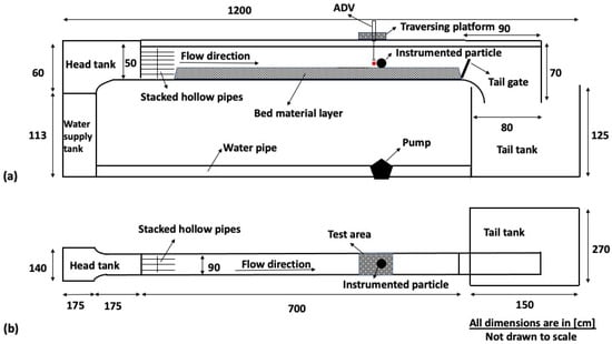
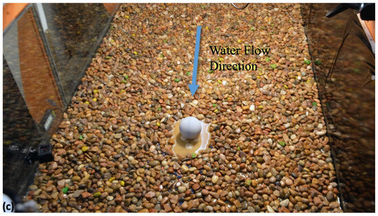
Figure 1.
Illustration of the experimental setup: (a) sketch of the side view of the flume, also showing the test section and the relevant instrumentation (acoustic Doppler velocimetry and the instrumented particle), (b) the top view and (c) photo from the experimental setup, illustrating the use of the instrumented particle sitting on top of a dedicated 3D-printed micro-topography, transferring entrainment data in real time via the WiFi protocol (effective for submergence depths below 13.5 cm—see the WiFi antenna attached on the frame above the target particle), the high-speed video camera (used for visually assessing particle entrainments from the side) and the instrumented particle. The flow direction is also shown.
Each run of the experiment consisted of performing the sensor measurements and flow velocity measurements. In general, there are two main approaches in assessing the relationship between the instantaneous flow hydrodynamic forcing (cause) and resulting particle entrainments (effect). This can be done deterministically, if the flow and particle instrumentation are synchronously taking records, or stochastically, by means of cross-examining the trends between these records, especially useful if these records have been taken separately but refer to the same particle and flow conditions. The use of the former deterministic in-synch records obtaining approach is only possible via the employment of non-intrusive velocimetry methods (such as laser Doppler velocimetry or particle image velocimetry). Given that the experiments carried herein use ADV, which can locally interfere with the particle, the latter stochastic assessment approach is used herein. This involves using the particle movement records towards indirectly inferring the flow impulses that are effective in entraining the instrumented particle, which are then stochastically compared to the directly measured flow hydrodynamics of the same flow. The particle entrainment and flow velocimetry records are obtained separately, having only one piece of instrumentation at a time to avoid either interfering with the other. In this manner, it is secured that there is no interference between the used instrumentation. The ADV is positioned 1 cm upstream of the face of the instrumented particle, and it is configured appropriately to record instantaneously the three components of the local flow field [55]. Flow velocity profiles are then taken after the instrumented particle has been removed, with a vertical resolution of about 7 mm. Likewise, the entrainment record of the instrumented particle is performed after the flow measurement instrumentation has been removed and can be obtained live (via the WiFi protocol) or otherwise saved in the local memory for retrieval after the conclusion of the flow experiment.
Five runs were performed, and the flow velocity measurements and the sensor measurements were used to investigate the flow structures that resulted in entraining the instrumented particle stochastically. For the stochastic analysis of particle entrainment, both the flow and particle entrainment time series are required to be long enough so that they have statistics that are representative and independent of the duration of the records. For the typical flow conditions assessed herein, such durations have been experimentally established to be 8 min for the ADV flow hydrodynamic records (12,000 samples at 25 Hz recording rate) and above half an hour for the instrumented particle entrainments records (more than 180,000 samples when recording at 100 Hz). These five runs were used for the analysis of the flow structures that occurred during, before and after the occurrence of impulses above the critical impulse. The acquired instantaneous flow velocity data were de-spiked using the methodology presented by Goring and Nikora [56], modified by Wahl [57] and Mori et al. [58]. The post-processed velocity measurements were then used to estimate the shear velocity () using the Grass method [10] as discussed in [54]. The shear velocity was used to estimate the particle Reynolds number and the Shields parameter for the five runs of the experiment. The results are shown in Section 3, Table 1.

Table 1.
The flow characteristics (mean flow velocity, mean flow depth, Froude number, flow and particle Reynolds number (Re and , respectively) and average bed surface Shields shear stresses) and resulting entrainment particle frequency for the 5 runs of the study.
The instantaneous flow velocity measurements 1 cm upstream of the instrumented particle’s face, in the longitudinal direction, and in the position in the middle of the top half of the particle’s diameter, in the bed-normal direction, were used as the input to the theoretical equations presented in [21,22], to estimate the flow impulses (as is also shortly illustrated, in Figure 2). This corresponds to point velocimetry taken at a fixed bed-normal distance from the bed surface, which ranges from about 1/3 to 2/5 of the flow depth. This position has been referred to as the position of investigation in this work. The quadrant analysis method was performed using the instantaneous flow velocity measurements at the position of the investigation. As presented in the introduction section, in the quadrant analysis method, the turbulent velocity fluctuations were divided into 4 categories, or quadrants, based on their signs: Q1 (+u′, +w′), Q2 (−u′, +w′), Q3 (−u′, −w′) and Q4 (+u′, −w′). The turbulent velocity fluctuations were estimated based on Equations (1) and (2) below:
where u and w are the instantaneous flow velocity readings (stream-wise and normal to the bed surface components), u′ and w′ are the turbulent velocity fluctuations (stream-wise and normal to the bed surface components), and are the time-averaged velocity (stream-wise and normal components) and i is the ADV instantaneous reading. Using each instantaneous velocity reading, or basic ADV reading, the quadrant that corresponds to the reading was defined. An illustration of the analysis that was performed using the flow velocity measurements to estimate the flow impulses and determine the quadrants is shown in Figure 2 below.
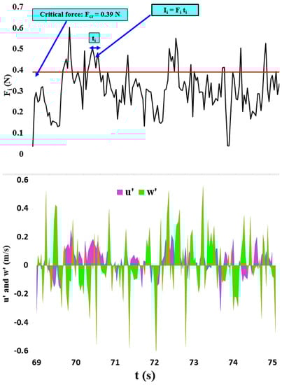
Figure 2.
Illustration of force versus time showing the critical force (Fcr = 0.39 N, shown as a horizontal red line), the temporal fluctuations of the stream-wise velocity fluctuating component at a certain location, and the temporal fluctuations of the bed-normal component of the flow velocity at a certain location (u′ and w′) versus time.
As discussed in [54], the frequency of entrainment of the instrumented particle was estimated using the normalised roll results by the inertial sensor fusion of the instrumented particle’s logged readings during the experiment. As for the flow impulses, which were estimated based on the illustration shown in Figure 2, they were used to estimate the frequency of flow impulses by dividing the total number of flow impulses by the total ADV recording time in each position, including the position of investigation. Given that the contribution of the Q2 and Q4 quadrants is more significant near the bed surface, it is expected that for smaller particle-size-to-flow-depth ratios, these quadrants will play a greater role in particle entrainment. Thus, it is expected that smaller particle sizes will have an even more pronounced contribution of the Q2 and Q4 events than found herein.
In the position of investigation, different theoretical critical impulse values (Icr) were tested to determine the value that results in a good agreement between the frequency of entrainment of the instrumented particle and the frequency of flow impulses above that value, or above the critical impulse (fI). Figure 3 below shows the selected critical value in addition to slightly higher and lower values for the critical impulse, for comparison purposes.
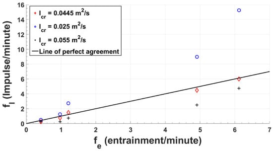
Figure 3.
The frequency of entrainment of the instrumented particle, estimated using its reading during the experiment, versus the frequency of flow impulses above the three different values of critical impulse. The continuous straight line shows the line of perfect agreement between the observed and predicted values (please note the vertical and horizontal axis have different scaling).
It is clear from Figure 3 that the critical impulse is very close to 0.0455 m2/s, i.e., the line of perfect agreement between the frequencies of flow impulses above the critical impulse and the frequency of entrainment of the instrumented particle. In a similar fashion, the theoretical equations presented in [21,22] can be used to derive values of critical impulses, by offering different input about the flow, grain and bed surface properties. and/or utilising appropriate assumptions (e.g., flow uniformity, grain shape, uniformity and packing of the bed surface grain sizes, local bed surface and grain arrangement slope). Due to dependence on all the above, there is no single reference value of the critical impulse that may set a grain into motion, but instead there is a range of flow conditions that may produce such results, depending on how frequently the generated flow impulses are in excess of the critical impulse level.
Based on the identified critical impulse value (0.0455 m2/s) and a chosen value (0.0063 m2/s) below the identified lower impulse bound (0.025 m2/s), the flow impulses that have resulted in entraining the instrumented particle are being examined stochastically. The reason a lower impulse value is also examined, is because a smaller critical value will produce the same but bigger magnitude impulses compared to the higher threshold critical impulse, for the same flow and bed surface hydrodynamics, but it will also generate a lot smaller magnitude and much more frequently occurring impulses, as shown in [22]. Thus, assessing the hydrodynamic interactions for a lower bound will allow offering a more conservative estimate for the effect of those flow structures on sediment transport. These are also expected to be of interest for the transport not only of sediment grains but also of smaller and/or more lightweight material (e.g., micro-plastics being caried along the fluvial vector) also exposed in the bed surface. Critically, assessing the occurrence of the different quadrant events and their sequence leading to entrainment, as validated via these bespoke flume experimental observations, is the overarching goal of this study. In the following section, the quadrants that occurred during, before and after the occurrence of flow impulses above the critical impulse were investigated in different windows of the ADV readings (1–5 readings).
3. Results
The flow depth, frequency of entrainment, particle Reynolds number and Shields parameter for the five runs of this study are shown in Table 1. It can easily be seen that while the flow depth is only slightly (e.g., less than 5%) changing with the increase of the flow rate, and the average shear stress eventually is less than doubling, the frequency of entrainments changes over an order of magnitude. This is to be expected for near threshold flow conditions and it also shows that the average flow metrics, such as mean bed surface shear stresses, are not sensitive in capturing the change in the probability of particle entrainment characterising the threshold flow conditions. Likewise, there is virtually no change for the mean flow velocities and Froude numbers, which illustrates that using equations which are indirectly employing mean flow parameters for assessing bed surface destabilisation or risk-to-scour around obstacles such as hydraulic infrastructure or instream vegetation is insufficient, while it could be directly done with instrumented particles [17].
The instrumented particle is only partially exposed to the flow, when the positioning of its local 3D-printed resting pocket relative to the top layers of bed surface particles is considered. The protrusion of the instrumented particle, defined as the ratio of the particle’s size seen by the flow over the flow depth, is assessed to be fixed at about 0.4. There have been many interesting studies assessing the role of particle protrusion into the flow e.g., [49], but here this is not further assessed given the infinitesimal changes of the flow depth relative to the particle’s protrusion ratio. This is currently being explored using a novel setup that allows the instrumented particle to remain mobile while changing its protrusion to the bed surface, as opposed to earlier studies e.g., [49], and will be reported in a separate study.
The first step that was performed in the analysis was checking the quadrant readings that have occurred in the flow for the period of the ADV recording in the position of investigation. This was in the middle of the top half of the instrumented particle. The results of the quadrant readings that occurred in the flow for the period of the ADV recording in the position of investigation are shown in Figure 4.
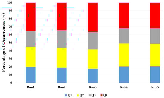
Figure 4.
The percentages of the quadrant readings that have occurred in the flow during the periods of the ADV recordings in the position of investigation for the five runs of the experiment.
The percentages of the quadrant readings that have occurred in the flow during the periods of ADV recordings in the position of investigation for the five runs of the experiment were almost the same with a slight dominance found in Q2 and Q4 (i.e., sweep and ejection events).
The next step of the analysis was investigating the quadrant readings that have occurred during the turbulent flow events with an impulse above the critical impulse. The results are shown in Figure 5 below.
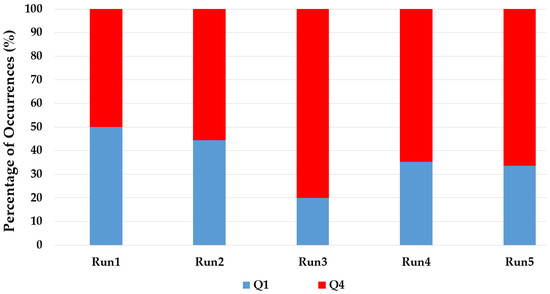
Figure 5.
The percentages of the quadrant readings that have occurred during the events with an impulse above the critical impulse (Icr = 0.0445 m2/s).
The impulse criterion only takes into account the turbulent flow events with a positive stream-wise velocity fluctuating component. The quadrant readings that have occurred during the events with an impulse above the critical impulse were Q1 and Q4 only, as is clear from Figure 5. The appearance of Q4 within the impulse above the critical impulse is more dominant than Q1 in the case of the three critical impulses of 0.0445 m2/s as is clear from Figure 5.
In the next step, the quadrants that have occurred before and after the occurrence of flow impulses above the critical impulse were investigated for the different windows of the readings (1–5 readings). The results are shown in Figure 6, Figure 7, Figure 8, Figure 9, Figure 10, Figure 11, Figure 12, Figure 13, Figure 14 and Figure 15.
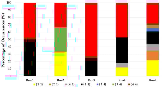
Figure 6.
The percentages of the transitions between 1 quadrant reading before the impulse above the critical impulse and the first quadrant reading during the impulse above the critical impulse (for Icr = 0.0445 m2/s).
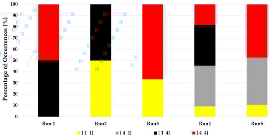
Figure 7.
The percentages of the transitions between the last quadrant reading during the impulse above the critical impulse and 1 quadrant reading after that (for Icr = 0.0445 m2/s).
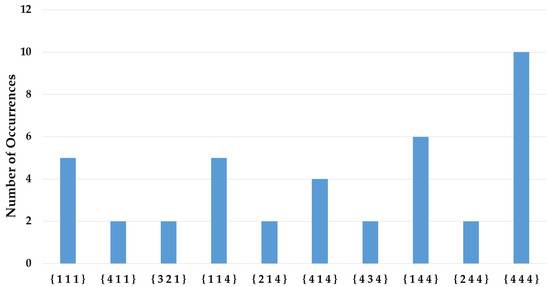
Figure 8.
The number of occurrences of the most dominant transitions between two quadrant readings before the impulse above the critical impulse and the first quadrant reading during the impulse above the critical impulse (for Icr = 0.0445 m2/s).
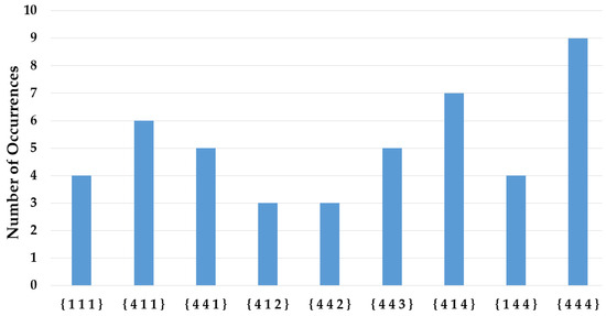
Figure 9.
The number of occurrences of the most dominant transitions between the last quadrant reading during the impulse above the critical impulse and two quadrant readings after that (for Icr = 0.0445 m2/s).
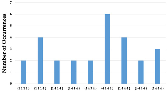
Figure 10.
The number of occurrences of the most dominant transitions between three quadrant readings before the impulse above the critical impulse and the first quadrant reading during the impulse above the critical impulse (for Icr = 0.0445 m2/s).
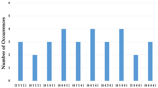
Figure 11.
The number of occurrences of the most dominant transitions between the last quadrant reading during the impulse above the critical impulse and three quadrant readings after that (for Icr = 0.0445 m2/s).
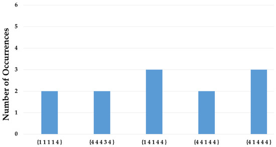
Figure 12.
The number of occurrences of the most dominant transitions between four quadrant readings before the impulse above the critical impulse and the first quadrant reading during the impulse above the critical impulse (for Icr = 0.0445 m2/s).
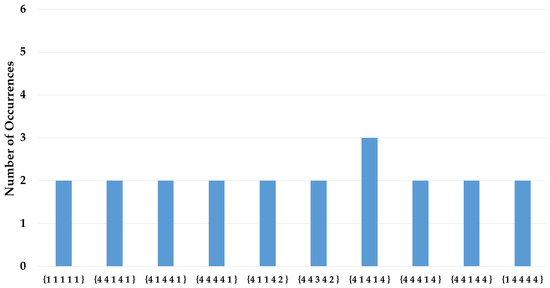
Figure 13.
The number of occurrences of the most dominant transitions between the last quadrant reading during the impulse above the critical impulse and four quadrant readings after that (for Icr = 0.0445 m2/s).
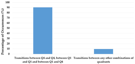
Figure 14.
The percentages of the transitions between five quadrant readings before the impulse above the critical impulse and the first quadrant reading during the impulse above the critical impulse (for Icr = 0.0445 m2/s).
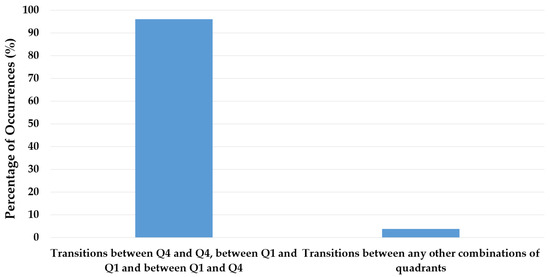
Figure 15.
The percentages of the transitions between the last quadrant reading during the impulse above the critical impulse and five quadrant readings after that (for Icr = 0.0445 m2/s).
It is clear from Figure 6 that in the case of the critical impulse of 0.0445 m2/s, most of the transitions between one quadrant reading before the occurrence of an impulse above the critical impulse and the first quadrant reading during the occurrence of an impulse above the critical impulse are between Q4 and Q4, Q1 and Q4 and Q1 and Q1. In the case of the transitions between the last quadrant reading during the occurrence of an impulse above the critical impulse and one quadrant reading after that, the result is between Q4 and Q4, Q1 and Q4 and Q1 and Q1, as it is clear from Figure 7. The same was observed for the case of transitions between two quadrant readings before and after the first and the last quadrant readings during the occurrences of impulses above the critical impulse. In other words, the transitions were between Q4 and Q4, Q1 and Q4 and Q1 and Q1, as shown in Figure 8 and Figure 9.
As Figure 10, Figure 11, Figure 12, Figure 13, Figure 14 and Figure 15 show, it is clear that most of the transitions between the first and the last quadrant readings during the occurrence of impulses above the critical impulse and three, four and five quadrants before and after these are again transitions between Q4 and Q4, Q1 and Q4 and Q1 and Q1.
The next step of the analysis that was performed was reducing the critical impulse to a value of 0.0063 m2/s similar to Valyrakis et al. [59]. This procedure was conducted to increase the number of impulses above the critical impulse and to provide more data for investigating the type of flow structure. In other words, the goal of this step was to investigate the events that are less energetic than the events that have been investigated previously, i.e., using the critical impulse value of 0.0455 m2/s, and assess their flow structures.
It is clear from Figure 16 that the occurrences of Q4 during the occurrences of impulses above the critical impulse are more dominant than Q1 in the case of a critical impulse of 0063 m2/s as is clear from Figure 15. This is a similar finding to the case of the critical impulse of 0.0445 m2/s.
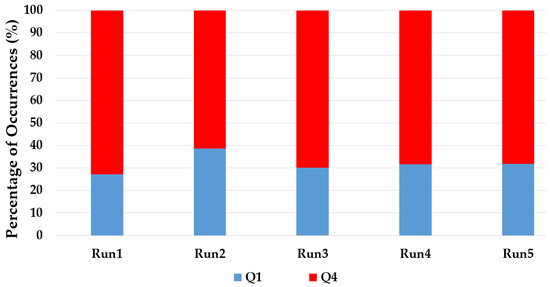
Figure 16.
The percentages of the quadrant readings that have occurred during the events with an impulse above the critical impulse (Icr = 0.0063 m2/s).
It is clear from Figure 17 that in the case of the critical impulse of 0.0063 m2/s, most of the transitions between one quadrant reading that has occurred before the occurrence of an impulse above the critical impulse and the first quadrant reading that has occurred during an impulse above the critical impulse are transitions between Q4 and Q4, Q1 and Q4 and Q1 and Q1. As for the case of the last quadrant reading that has occurred during the occurrence of an impulse above the critical impulse and one quadrant reading that has occurred after that, most are transitions between Q4 and Q4, Q1 and Q4 and Q1 and Q1 as is clear from Figure 18. This is the similar observation to the case of transitions between one quadrant before and one quadrant after the first and the last quadrants that have occurred during the occurrence of impulses above the critical impulse. Another observation that could be made is that there is a slight increase in the transitions between Q2 and Q4 and Q3 and Q4 that have occurred one quadrant before and after the first and the last quadrant readings that have occurred during the occurrence of an impulse above the critical impulse. Similar to the case of a critical impulse of 0.0445 m2/s, it could be observed that in the case of transitions between two quadrant readings before and after the first and the last quadrant reading, they have occurred during the impulse above the critical impulse. In other words, the transitions are between Q4 and Q4, Q1 and Q4 and Q1 and Q1 as shown in Figure 19 and Figure 20.
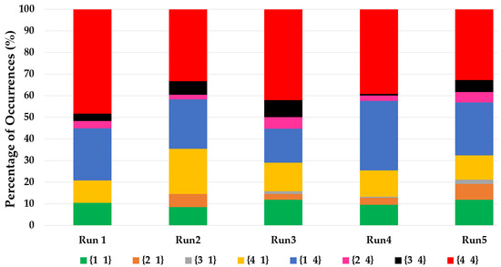
Figure 17.
The percentages of the transitions between 1 quadrant reading before the impulse above the critical impulse and the first quadrant reading during the impulse above the critical impulse (for Icr = 0.0063 m2/s).
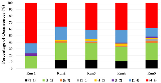
Figure 18.
The percentages of the transitions between the last quadrant reading during the impulse above the critical impulse and 1 quadrant reading after that (for Icr = 0.0063 m2/s).
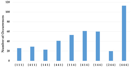
Figure 19.
The percentages of the occurrences of the most dominant transitions between two quadrant readings before the impulse above the critical impulse and the first quadrant reading during the impulse above the critical impulse (for Icr = 0.0063 m2/s).
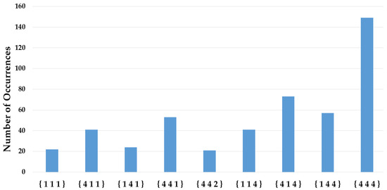
Figure 20.
The percentages of the occurrence of the most dominant transitions between the last quadrant reading during the impulse above the critical impulse and 2 quadrant readings after that (for Icr = 0.0063 m2/s).
Finally, according to Figure 21 and Figure 22, it is clear that most of the transitions between the first and last quadrant reading occurred during an impulse above the critical impulse and three, four and five quadrants before and after that are transitions between Q4 and Q4, Q1 and Q4 and Q1 and Q1.
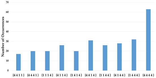
Figure 21.
The percentages of the occurrences of the most dominant transitions between three quadrant readings before the impulse above the critical impulse and the first quadrant reading during the impulse above the critical impulse (for Icr = 0.0063 m2/s).
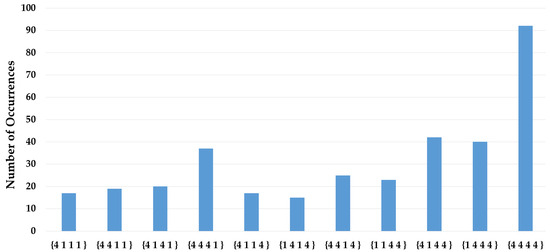
Figure 22.
The percentages of the occurrence of the most dominant transitions between the last quadrant reading during the impulse above the critical impulse and 3 quadrant readings after that (for Icr = 0.0063 m2/s).
4. Discussion
In this work, the frequency of entrainment of the instrumented particle, 7 cm in diameter, that was estimated using its logged readings, is linked to the frequency of flow impulses above the critical impulse at the positions in the middle of the top half of the particle’s diameter, which is the position of investigation. Different threshold values were assessed to determine the critical impulse that results in a good agreement between the frequencies of entrainment of the instrumented particle, estimated using its readings, and the flow impulses above the critical impulse as shown in Figure 2. The main aim of this study was to assess whether there was any trend in terms of the type of flow structures that occur in sequence before and after the occurrences of the flow impulses that have resulted in the coarse particle’s entrainment.
The ADV logging frequency that was used in the experiment of this work for flow velocity measurements was 25 Hz. The ADV was able to detect events with a timescale of 0.04 s and higher. Based on the conclusion of the experimental work of Valyrakis et al. (2013), more than 50% of the turbulent flow events that have resulted in the dislodgement of the particle that was used in their research in the stream-wise direction have length scales of the particle’s diameter. Additionally, only a very small fraction of the turbulent flow events that have resulted in the dislodgement of the coarse particle that was used in the stream-wise direction have length scales four times the particle’s diameter. Hofland et al. [48] reported a similar observation, specifically that the length scale of the events that have resulted in sediment entrainment are sweeps of two to four grain diameters in the stream-wise direction.
In the experiment in this work, the instrumented particle that was used was 7 cm in diameter. The critical velocity used to overcome the resistance and to entrain the instrumented particle that was placed on the micro-topography used in this experiment, based on the moment balance equations [21], was 0.623 m/s. Therefore, assuming the length scale of a turbulent flow event of the coarse particle’s diameter, the mean time scale of such an event could be estimated using Equation (3):
where is the time-scale of the turbulent flow event.
The ADV that was used in the experiment of this work for flow velocity measurements has a logging frequency of 25 Hz, therefore it was able to detect turbulent flow events of length scales of 35% of the particle’s diameter and longer, assuming their velocities are equal to the critical velocity. Therefore, the logging frequency of the ADV used in this work is sufficient for the study of coherent flow structures that can result in the entrainment of the instrumented particle placed on the micro-topography used in this work based on the conclusions of the experimental work presented in [22,48]. Further investigation was performed by assessing the histogram of the durations of the impulses above the critical impulse (Icr = 0.0445 m2/s), as shown in Figure 23 below.
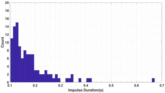
Figure 23.
Histogram of the durations of the flow impulses for all five runs of the experiment (for Icr = 0.0445 m2/s).
Close investigation of the histogram of the durations of impulses above 0.0445 m2/s indicates that about 75% of the impulses have durations of less than 0.2 s. This duration, 0.2 s, is equivalent to five ADV readings. Therefore, it has been decided to investigate the quadrant readings for a window of 1–5 readings in the case of Icr = 0.0445 m2/s.
Another investigation that was performed was lowering the critical impulse to a value of 0.0063 m2/s. This is similar to the critical impulse used by Valyrakis et al. [59]. This procedure increases the number of impulses above the critical impulse and provides more data for the quadrant analysis. To define the window of investigation of the quadrant readings for the case of Icr = 0.0063 m2/s, the histogram of the durations of the impulses above the critical impulse, Figure 24, was assessed.
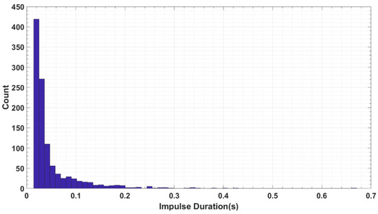
Figure 24.
Histogram of the durations of the flow impulses for all five runs of the experiment (for Icr = 0.0063 m2/s).
Close investigation of the histogram of the durations of impulses above 0.0063 m2/s indicates that about 90% of the impulses have durations of less than 0.12 s. This duration, 0.12 s, is equivalent to up to three ADV readings. Therefore, it has been decided to investigate the quadrant readings for a window of the first few readings, in the case of Icr = 0.0063 m2/s. The mean time scale of the flow structure that is of comparable size to the instrumented particle, and thought to be relevant to its entrainment [21], has been identified in Equation (3). The authors of [21] have shown that at near threshold flow conditions, the impulses that may lead to coarse particle entrainment have timescales that correspond to about 1–3 times the particle’s representative length-scale (diameter). Thus, in our analysis it is considered that the near threshold impulse events are mostly short-lived and as a consequence better represented by a sequence of one or two readings (given the ADV recording frequency and the entrainment inducing impulses). We could also be assessing sequences of three or more readings, but these would primarily correspond to impulses above critical, much less than threshold and near threshold impulses that are relatively more long-lived (e.g., only a small percentage according to [21,22]).
As for the quadrant readings in the flow, it is clear from Figure 4 that there is a slight dominance in the occurrences of Q4 and Q2 quadrant readings in comparison to the occurrences of Q1 and Q3 quadrant readings in the flow. This is similar to some of the observations that have been reported in the literature for a similar type of flow (Cantwell, 1981; Robinson, 1991b). As for the quadrant readings within the impulses, sweeps have occurred more than outward interactions during the events with impulses above the critical impulse (for both cases Icr = 0.0445 m2/s and Icr = 0.0063 m2/s) as can be noticed from Figure 5 and Figure 16. The difference between the percentages of occurrence of Q4 readings and Q1 readings in the flow (shown in Figure 4) does not justify the difference between the percentages of the occurrences of Q4 and Q1 during the events with impulses above the critical impulse. This conclusion is similar to the findings of Nelson et al. [43], i.e., Q4 moves the majority of the sediment followed by Q1 and to a much lesser extent, Q2 and Q3. However, according to Nelson et al. [43], the main reason that Q4 moves the majority of the sediment compared to Q1 is due to its common occurrence. This is not the case in this study. In other words, and as is clear from Figure 4, for the five runs of the experiment, the percentages of quadrant readings that have occurred in the flow during the periods of ADV recordings at the position of investigation are almost the same with the slight dominance of Q2 and Q4 (i.e., sweep and ejection events). Dwivedi et al. [47] suggested that a higher probability of occurrence of a high-magnitude force is induced by sweep events.
Of importance is to observe that even though the Q2 and Q4 events are somewhat more commonly observed than the Q1 and Q3 events (Figure 4), the majority of the high magnitude impulses are due to Q4 events (according to e.g., Figure 5). A possible explanation for this is due to the much higher magnitude of the Q2 and Q4 events compared to the Q1 and Q3 events, eventually resulting at higher stress values [60,61]. This can be clearly seen for example from the joint probability distributions of the velocity component fluctuations (u′ and v′), according to Wallace [60,62]. The joint probability distribution has an elliptical shape which is significantly more elongated in the Q2 and Q4 quadrants. As a consequence, the Q2 and Q4 events are having more high magnitude values while the Q1 and Q3 events will be limited to relatively smaller magnitude values. This observation aligns with the fact that impulses above a critical level, linked to entrainments, should be of a higher value, thus the contribution of the higher magnitude Q4 events will be more pronounced compared to the Q1 events.
Additionally, Dey et al. [63] suggested that sweeps are the more dominant mechanism in sediment entrainment while Q4 and Q2 cancel each other out on an immobile bed, giving rise to the Q1. Other researchers [12,64] have also reported the predominance of the role of Q4 and to a lesser extent Q1 in sediment entrainment. According to the rest of the figures in the results section, considering all five runs, for both cases of critical impulse, i.e., Icr = 0.0445 m2/s and Icr = 0.0063 m2/s, for both investigation windows of readings, i.e., 1–5 readings and 1–3 readings and for before and after the occurrences of impulses above the critical impulse, it is clear that most of the transitions between the quadrant readings are Q4 to Q4, Q1 to Q4 and Q1 to Q1. In other words, it is clear from the results of this study that the impulses above the critical impulse, i.e., the impulses that have caused the instrumented particle’s entrainment, are relatively short-lived sweep events and to a lesser extent, relatively short-lived outward interactions. This conclusion is supported by the observation that the majority of transitions between quadrant readings occur before and after the first and last quadrant readings of the impulses above the critical impulse being Q4 to Q4 and Q1 to Q1. This is in addition to the transitions between sweeps and outward interactions, i.e., Q4 and Q1.
The presence of even a weak but non-negligible secondary flow in a rectangular flume can affect the structure and intensity of the shear flow and subsequently influence the probability of sediment entrainment rates. Secondary flow is significantly affected via the flume’s aspect ratio. In this study, the aspect ratio of the rectangular channel for the flows tried, is about 8.2 and it is almost fixed, given that the flow depth is changing less than 5%. Jing et al. [65], assessed the impact of secondary flow in an open channel for ratios ranging from 3 to 7.5 and found the presence of more secondary flow cells for the higher aspect ratios, which is also closer to the aspect ratio in our experiment. These can affect the flow velocity and flow energy distribution, resulting for example in possible deviations from the mean logarithmic flow velocity profiles, which we have also observed. These are expected to change as the aspect ratio of the flume is altered but given its infinitesimal change for the flow rates trialled herein, it is expected that any contribution of secondary flows to the entrainment rate of the target coarse particle, will remain the same.
Finally, do the impulses correspond to coherent flow structures and vice versa? The answer to that is yes and no. An impulse includes the magnitude and duration of the turbulent flow events. However, the impulse criterion is a resistance dependent criterion. If the resistance is small, small fluctuations can result in particle entrainment but if the resistance is big, the small fluctuations cannot result in the entraining of a particle. In other words, for the same flow field, having two particles of different diameters results in a different distribution of impulses, even though the same distribution of coherent flow structures exists in the flow field. Thus, for a non-uniform bed surface, having a range of entrainment resistance thresholds, the amount of overlap between the instantaneous hydrodynamic forcing (represented by the distribution of impulses above critical), assessed for the different critical impulses (representing the distinct resistance levels), will be indicative of the probability of entrainment. However, closer to the bed surface the contribution of Q2 and Q4 events may increase, which leaves more space for future research to explore how the contribution of these quadrants may change for different particle-size-to-flow-depth ratios (i.e., grain bed surface exposure ratios).
5. Conclusions
In this work, an instrumented particle of 7 cm has been used to investigate the incipient entrainment from a hydraulically rough bed surface. Five runs of a well-controlled laboratory flume experiment were performed for a flowrate range near the critical threshold of motion. ADV was used to record the local flow hydrodynamics from which flow impulses above critical can be estimated, as well as define the quadrant that each reading corresponds to. The critical impulse level herein was defined by stochastically linking the frequency of a coarse instrumented particle entrainment estimated using the sensor readings, to the frequency of the flow impulses above the critical impulse for each corresponding critical impulse level. The main objective of this study was to identify trends in the sequence of flow structures before and after the occurrence of impulses in excess of the critical level, linked to coarse particle entrainment, using quadrant analysis.
Our results indicate that there is a slight dominance in the Q4 and Q2 quadrant events compared to the Q1 and Q3 quadrant readings, in the flow. Additionally, sweep quadrant readings have occurred more often compared to outward interaction quadrant events during the occurrence of impulses above the critical level. However, given the greater prevalence of Q2 and Q4 events near the bed surface, it is expected that for cases of smaller particle-size-to-flow-depth ratios, these events will contribute even more towards coarse particle entrainment.
Finally, the results, considering all five runs, indicate the primary contribution of sweep events (Q4 to Q4, Q1 to Q4) and secondarily the ejection events (Q1 to Q1, for both cases of critical impulse, i.e., Icr = 0.0445 m2/s and Icr = 0.0063 m2/s). In essence, the findings of this study clearly demonstrate that the impulses above the critical impulse, which are responsible for the entrainment of the coarse instrumented particle, predominantly consist of relatively short-lived sweep events and to a lesser extent, relatively short-lived outward interactions. This conclusion is confirmed by the finding that the bulk of quadrant reading transitions take place prior to and following the first and last quadrant readings of the impulses. This is in addition to the transitions between sweeps and outward interactions, i.e., Q4 and Q1.
Author Contributions
Conceptualization, M.V.; methodology, M.V. and K.A.; software, K.A. and M.V.; validation, M.V. and K.A.; formal analysis, K.A.; investigation, K.A.; resources, K.A.; data curation, M.V. and K.A.; writing—original draft preparation, K.A.; writing—review and editing, M.V. and K.A.; visualization, M.V. and K.A.; supervision, M.V.; project administration, M.V.; funding acquisition, M.V. All authors have read and agreed to the published version of the manuscript.
Funding
This work has been supported in part by the Royal Society (Research Grant RG2015 R1 68793/1), the Royal Society of Edinburg (Crucible Award) and the Carnegie Trust for the Universities of Scotland (project 7066215).
Data Availability Statement
All data are available in the main text body and can be made available upon submitting a request to the corresponding author.
Acknowledgments
We are grateful to the University of Glasgow lab technician, Timothy Montgomery, and undergraduate research student, Athanasios (Thanos) Alexakis, for their help in preparing the experimental setup, as well as the editor and the anonymous reviewers for their recommendations.
Conflicts of Interest
The authors declare no conflict of interest.
References
- Gomez, B.; Church, M. An assessment of bed load sediment transport formulae for gravel bed rivers. Water Resour. Res. 1989, 25, 1161–1186. [Google Scholar] [CrossRef]
- Leopold, L.B.; Emmett, W.W. Bedload measurements, East Fork River, Wyoming. Proc. Natl. Acad. Sci. USA 1976, 73, 1000–1004. [Google Scholar] [CrossRef]
- Talukdar, S.; Kumar, B.; Dutta, S. Predictive Capability of Bedload Equations Using Flume Data. J. Hydrol. Hydromech. 2012, 60, 45–56. [Google Scholar] [CrossRef][Green Version]
- Shields, A. Application of Similarity Principles and Turbulence Research to Bed-Load Movement; California Institute of Technology: Pasadena, CA, USA, 1936. [Google Scholar]
- Bagnold, R.A. An Approach to the Sediment Transport Problem from General Physics; Physiographic and Hydraulic Studies of Rivers, Geological Survey Professional Paper 422-I; United States Government Printing Office: Washington, DC, USA, 1966; pp. 1–37.
- Bagnold, R.A. Transport of solids by natural water flow: Evidence for a worldwide correlation. Proc. R. Soc. Lond. A Math. Phys. Sci. 1986, 405, 369–374. [Google Scholar]
- Reynolds, O. On the dynamical theory of incompressible viscous fluids and the determination of the criterion. Philos. Trans. R. Soc. Lond. A 1895, 186, 123–164. [Google Scholar]
- Einstein, H.A.; El-Samni, E.A. Hydrodynamic forces on a rough wall. Pap. Present. Rev. Mod. Phys. 1949, 21, 520–524. [Google Scholar] [CrossRef]
- Einstein, H.A. The Bed-Load Function for Sediment Transportation in Open Channel Flows. (Technical Report No. 1026). United States Department of Agriculture, Soil Conservation Service. 1950. Available online: https://naldc.nal.usda.gov/download/CAT86201017/PDF (accessed on 1 January 2020).
- Grass, A.J. Initial Instability of Fine Bed Sand. J. Hydraul. Div. 1970, 96, 619–632. [Google Scholar] [CrossRef]
- Grass, A.J. Structural features of turbulent flow over smooth and rough boundaries. J. Fluid Mech. 1971, 50, 233–255. [Google Scholar] [CrossRef]
- Heathershaw, A.D.; Thorne, D.P. Seabed noises reveal role of turbulent bursting phenomenon in sediment transport by tidal currents. Nature 1985, 316, 339–342. [Google Scholar] [CrossRef]
- Leighly, J.B. Turbulence and the transportation of rock debris by streams. Geogr. Rev. 1934, 24, 453–464. [Google Scholar] [CrossRef]
- Sutherland, A.J. Proposed mechanism for sediment entrainment by turbulent flows. J. Geophys. Res. 1967, 72, 6183–6194. [Google Scholar] [CrossRef]
- Schmeeckle, M.W.; Nelson, J.M. Direct numerical simulation of bedload transport using a local, dynamic boundary condition. Sedimentology 2003, 50, 279–301. [Google Scholar] [CrossRef]
- Sumer, B.M.; Lloyd HC, C.; Cheng, N.S.; Fredsøe, J. Influence of Turbulence on Bed Load Sediment Transport. J. Hydraul. Eng. 2003, 129, 585–596. [Google Scholar] [CrossRef]
- Xu, Y.; Valyrakis, M.; Gilja, G.; Michalis, P.; Yagci, O.; Przyborowski, L. Assessing riverbed surface destabilization risk downstream isolated vegetation elements. Water 2022, 14, 2880. [Google Scholar] [CrossRef]
- Williams, J.J.; Thorne, P.D.; Heathershaw, A.D. Measurements of turbulence in the benthic boundary layer over a gravel bed. Sedimentology 1989, 36, 959–971. [Google Scholar] [CrossRef]
- Diplas, P.; Dancey, C.L.; Celik, A.O.; Valyrakis, M.; Greer, K.; Akar, T. The Role of Impulse on the Initiation of Particle Movement Under Turbulent Flow Conditions. Science 2008, 322, 717–720. [Google Scholar] [CrossRef]
- Valyrakis, M.; Diplas, P.; Dancey, C.L.; Greer, K.; Celik, A.O. Role of instantaneous force magnitude and duration on particle entrainment. J. Geophys. Res. Earth Surf. 2010, 115, 1–18. [Google Scholar] [CrossRef]
- Celik, A.O.; Diplas, P.; Dancey, C.L.; Valyrakis, M. Impulse and particle dislodgement under turbulent flow conditions. Phys. Fluids 2010, 22, 046601. [Google Scholar] [CrossRef]
- Valyrakis, M.; Diplas, P.; Dancey, C.L. Entrainment of coarse particles in turbulent flows: An energy approach. J. Geophys. Res. Earth Surf. 2013, 118, 53. [Google Scholar] [CrossRef]
- Kline, S.J.; Reynolds, W.C.; Schraub, F.A.; Runstadler, P.W. The structure of turbulent boundary layers. J. Fluid Mech. 1967, 30, 741–773. [Google Scholar] [CrossRef]
- Adrian, R.J. Hairpin vortex organization in wall turbulence. Phys. Fluids 2007, 19, 041301. [Google Scholar] [CrossRef]
- Robinson, S.K. Coherent Motions in the Turbulent Boundary Layer. Annu. Rev. Fluid Mech. 1991, 23, 601–639. [Google Scholar] [CrossRef]
- Smith, C. Coherent flow structures in smooth-wall turbulent boundary layers: Facts, mechanisms and speculation. In Coherent Flow Structures in Open Channels; Ashworth, P.J., Ed.; J. Wiley: Chichester, UK, 1996; pp. 1–39. [Google Scholar]
- AlHusban, Z.; Valyrakis, M. Assessing sediment transport dynamics from energy perspective by using the smart sphere. Int. J. Sediment Res. 2022, 37, 833–846. [Google Scholar] [CrossRef]
- Wallace, J.M.; Eckelmann, H.; Brodkey, R.S. The wall region in turbulent shear flow. J. Fluid Mech. 1972, 54, 39–48. [Google Scholar] [CrossRef]
- Corino, E.R.; Brodkey, R.S. A visual investigation of the wall region in turbulent flow. J. Fluid Mech. 1969, 37, 1–30. [Google Scholar] [CrossRef]
- Best, J. On the entrainment of sediment and initiation of bed defects: Insights from recent developments within turbulent boundary layer research. Sedimentology 1992, 39, 797–811. [Google Scholar] [CrossRef]
- Cleaver, J.W.; Yates, B. The effect of re-entrainment on particle deposition. Chem. Eng. Sci. 1976, 31, 147–151. [Google Scholar] [CrossRef]
- Dyer, K.R.; Soulsby, R.L. Sand Transport on the Continental Shelf. Annu. Rev. Fluid Mech. 1988, 20, 295–324. [Google Scholar] [CrossRef]
- Grass, A.J. The influence of boundary layer turbulence on the mechanics of sediment transport. In Mechanics of Sediment Transport; Müller, A., Mutlu Sumer, B., Euromech Colloquium, Eds.; Balkema: Rotterdam, The Netherlands, 1983. [Google Scholar]
- Kaftori, D.; Hetsroni, G.; Banerjee, S. The effect of particles on wall turbulence. Int. J. Multiph. Flow 1998, 24, 359–386. [Google Scholar] [CrossRef]
- Lapointe, M. Burst-like sediment suspension events in a sand bed river. Earth Surf. Process. Landf. 1992, 17, 253–270. [Google Scholar] [CrossRef]
- Nakagawa, H.; Nezu, I. Prediction of the contribution to Reynolds stress from bursting events in open-channel flow. J. Fluid Mech. 1977, 80, 99–128. [Google Scholar] [CrossRef]
- Ninto, Y.; Garcia, M.H. Experiments on particle—Turbulence interactions in the near–wall region of an open channel flow: Implications for sediment transport. J. Fluid Mech. 1996, 326, 285–319. [Google Scholar] [CrossRef]
- Rashidi, M.; Hetsroni, G.; Banerjee, S. Particle-turbulence interaction in a boundary layer. Int. J. Multiph. Flow 1990, 16, 935–949. [Google Scholar] [CrossRef]
- Sechet, P.; Le Guennec, B. Bursting phenomenon and incipient motion of solid particles in bed-load transport. J. Hydraul. Res. 1999, 37, 683–696. [Google Scholar] [CrossRef]
- Sumer, B.M.; Deigaard, R. Particle motions near the bottom in turbulent flow in an open channel. Part 2. J. Fluid Mech. 1981, 109, 311–337. [Google Scholar] [CrossRef]
- Cantwell, B.J. Organized Motion in Turbulent Flow. Annu. Rev. Fluid Mech. 1981, 13, 457–515. [Google Scholar] [CrossRef]
- Jiménez, J. Turbulent flows over rough walls. Annu. Rev. Fluid Mech. 2004, 36, 173–196. [Google Scholar] [CrossRef]
- Nelson, J.M.; Shreve, R.L.; McLean, S.R.; Drake, T.G. Role of Near-Bed Turbulence Structure in Bed Load Transport and Bed Form Mechanics. Water Resour. Res. 1995, 31, 2071–2086. [Google Scholar] [CrossRef]
- Celik, A.O.; Diplas, P.; Dancey, C.L. Instantaneous turbulent forces and impulse on a rough bed: Implications for initiation of bed material movement. Water Resour. Res. 2013, 49, 2213–2227. [Google Scholar] [CrossRef]
- Detert, M.; Nikora, V.; Jirka, G.H. Synoptic velocity and pressure fields at the water–sediment interface of streambeds. J. Fluid Mech. 2010, 660, 55–86. [Google Scholar] [CrossRef]
- Dwivedi, A.; Melville, B.; Shamseldin, A.Y. Hydrodynamic Forces Generated on a Spherical Sediment Particle during Entrainment. J. Hydraul. Eng. 2010, 136, 756–769. [Google Scholar] [CrossRef]
- Dwivedi, A.; Melville, B.W.; Shamseldin, A.Y.; Guha, T.K. Flow structures and hydrodynamic force during sediment entrainment. Water Resour. Res. 2011, 47, 1–18. [Google Scholar] [CrossRef]
- Hofland, B.; Battjes, J.; Booij, R. Measurement of Fluctuating Pressures on Coarse Bed Material. J. Hydraul. Eng. 2005, 131, 770–781. [Google Scholar] [CrossRef]
- Schmeeckle, M.W.; Nelson, J.M.; Shreve, R.L. Forces on stationary particles in near-bed turbulent flows. J. Geophys. Res. Earth Surf. 2007, 112, 1–21. [Google Scholar] [CrossRef]
- Smart, G.M.; Habersack, H.M. Pressure fluctuations and gravel entrainment in rivers. J. Hydraul. Res. 2007, 45, 661–673. [Google Scholar] [CrossRef]
- Paiement-Paradis, G.; Buffin-Bélanger, T.; Roy, A.G. Scalings for large turbulent flow structures in gravel-bed rivers. Geophys. Res. Lett. 2003, 30, 1773. [Google Scholar] [CrossRef]
- AlObaidi, K.; Xu, Y.; Valyrakis, M. The Design and Calibration of Instrumented Particles for Assessing Water Infrastructure Hazards. J. Sens. Actuator Netw. 2020, 9, 36. [Google Scholar] [CrossRef]
- AlObaidi, K.; Valyrakis, M. A sensory instrumented particle for environmental monitoring applications: Development and calibration. IEEE Sens. 2021, 21, 10153–10166. [Google Scholar] [CrossRef]
- AlObaidi, K.; Valyrakis, M. Linking the explicit probability of entrainment of instrumented particles to flow hydrodynamic. Earth Surf. Process. Landf. 2021, 46, 2448–2465. [Google Scholar] [CrossRef]
- Liu, D.; AlObaidi, K.; Valyrakis, M. The assessment of an Acoustic Doppler Velocimetry profiler from a user’s perspective. Acta Geophys. 2022, 70, 2297–2310. [Google Scholar] [CrossRef]
- Goring, D.G.; Nikora, V.I. Despiking Acoustic Doppler Velocimeter Data. J. Hydraul. Eng. 2002, 128, 117–126. [Google Scholar] [CrossRef]
- Wahl, T. Discussion of “Despiking Acoustic Doppler Velocimeter Data” by Derek G. Goring and Vladimir I. Nikora. J. Hydraul. Eng. 2003, 129, 484–487. [Google Scholar] [CrossRef]
- Mori, N.; Suzuki, T.; Kakuno, S. Noise of Acoustic Doppler Velocimeter Data in Bubbly Flows. J. Eng. Mech. 2007, 133, 122–125. [Google Scholar] [CrossRef]
- Valyrakis, M.; Diplas, P.; Dancey, C.L. Entrainment of coarse grains in turbulent flows: An extreme value theory approach. Water Resour. Res. 2011, 47, 1–17. [Google Scholar] [CrossRef]
- Wallace, J.M. Quadrant Analysis in Turbulence Research: History and Evolution. Annu. Rev. Fluid Mech. 2016, 48, 131–158. [Google Scholar] [CrossRef]
- Raupach, M.R. Conditional statistics of Reynolds stress in rough-wall and smooth-wall turbulent boundary layers. J. Fluid Mech. 1981, 108, 363–382. [Google Scholar] [CrossRef]
- Wallace, J.M.; Brodkey, R.S. Reynolds stress and joint probability density distributions in the u-v plane of a turbulent channel flow. Phys. Fluids 1977, 20, 351–355. [Google Scholar] [CrossRef]
- Dey, S.; Sarkar, S.; Solari, L. Near-Bed Turbulence Characteristics at the Entrainment Threshold of Sediment Beds. J. Hydraul. Eng. 2011, 137, 945–958. [Google Scholar] [CrossRef]
- Cecchetto, M.; Tregnaghi, M.; Bottacin-Busolin, A.; Tait, S.; Marion, A. Statistical Description on the Role of Turbulence and Grain Interference on Particle Entrainment from Gravel Beds. J. Hydraul. Eng. 2017, 143, 06016021. [Google Scholar] [CrossRef]
- Jing, S.; Yang, W.; Chen, Y. Smooth Open Channel with Increasing Aspect Ratio: Influence on Secondary Flow. Water 2019, 11, 1872. [Google Scholar] [CrossRef]


Disclaimer/Publisher’s Note: The statements, opinions and data contained in all publications are solely those of the individual author(s) and contributor(s) and not of MDPI and/or the editor(s). MDPI and/or the editor(s) disclaim responsibility for any injury to people or property resulting from any ideas, methods, instructions or products referred to in the content. |
© 2023 by the authors. Licensee MDPI, Basel, Switzerland. This article is an open access article distributed under the terms and conditions of the Creative Commons Attribution (CC BY) license (https://creativecommons.org/licenses/by/4.0/).