On the Finite Element Modeling of the Lumbar Spine: A Schematic Review

Vincenza Sciortino; Salvatore Pasta; Tommaso Ingrassia; Donatella Cerniglia

doi:10.3390/app13020958

,

and

¹

Department of Engineering, University of Palermo, Viale delle Scienze, 90128 Palermo, Italy

²

Department of Research, Istituto di Ricovero e Cura a Carattere Scientifico-Istituto Mediterraneo per i Trapianti e Terapie ad Alta Specializzazione (IRCCS-ISMETT), 90100 Palermo, Italy

^*

Author to whom correspondence should be addressed.

Appl. Sci.2023, 13(2), 958;https://doi.org/10.3390/app13020958

This article belongs to the Special Issue Feature Review Papers in Section Applied Biosciences and Bioengineering

Version Notes

Order Reprints

Abstract

Finite element modelling of the lumbar spine is a challenging problem. Lower back pain is among the most common pathologies in the global populations, owing to which the patient may need to undergo surgery. The latter may differ in nature and complexity because of spinal disease and patient contraindications (i.e., aging). Today, the understanding of spinal column biomechanics may lead to better comprehension of the disease progression as well as to the development of innovative therapeutic strategies. Better insight into the spine’s biomechanics would certainly guarantee an evolution of current device-based treatments. In this setting, the computational approach appears to be a remarkable tool for simulating physiological and pathological spinal conditions, as well as for various aspects of surgery. Patient-specific computational simulations are constantly evolving, and require a number of validation and verification challenges to be overcome before they can achieve true and accurate results. The aim of the present schematic review is to provide an overview of the evolution and recent advances involved in computational finite element modelling (FEM) of spinal biomechanics and of the fundamental knowledge necessary to develop the best modeling approach in terms of trustworthiness and reliability.

Keywords:

finite element analysis; spinal column; biomechanics; modelling; lumbar spine; computational simulations

1. Introduction

The study of spine biomechanics has evolved over decades. Computational simulations provide a critical tool in light of the difficulty and complexity required to perform in vivo experiments on human spinal columns [,,]. The biomechanics of the spine are extremely complex, and many different anatomical components are involved. In computational simulations, these components are modelled separately, each one being associated with specified modelling features according to their biomechanical response and constitutive model relationships [,]. A complete finite element (FE) analysis of the spine requires the modelling of bone components, intervertebral discs, facet joints, and seven major spinal ligaments, as well as the cartilaginous endplates [,,,].

The bone component consists of three parts: the cancellous bone (the innermost part), cortical bone (the outermost part), and posterior bony elements (which represent the vertebral arch where the bone marrow is inserted) []. The intervertebral disc is divided into the nucleus pulposus and the fibrous annulus, composed of the annular ground substance and reinforcing fibers. The three distinct parts of the disc should be modelled to simulate the correct biomechanics of the spinal column [,]. Therefore, the facet joint needs to be represented in order to account for the relative movement between the spinal processes of the two vertebrae. The seven major ligaments represented in the FE model are the anterior longitudinal ligament (ALL), posterior longitudinal ligament (PLL), interspinous ligament (IL), intertransverse ligament (TL), flavian ligament (FL), supraspinous ligament (SL), and capsular ligament (CL) [,]. Ligaments contribute to spinal stabilization by establishing the follower force path-way, which passes through the rotation centers of the vertebrae [,,,]. In an FE model of the lumbar spine, all these different components must be considered and modelled in order to ensure that the model is as reliable as possible. Dreisharf et al. [] compared eight different finite element studies [,,,,,,,] of the spine in a very comprehensive study. The eight element models were chosen according to the importance of the research carried out by the authors. The aim of the comparison was to observe whether it was possible to develop a prediction model of the lumbar spine’s behaviour under certain loading conditions. From the different studies, a certain homogeneity and average of the results was observed. This homogeneity was achieved as a result of the correct and complex modelling of the different anatomical parts modelled by the authors in a comprehensive manner.

The target of most biomechanical spine simulations is to evaluate the spinal loading conditions under physiological and pathological conditions [,,]. Intradiscal pressure (IDP) and displacement measurements are the main parameters for analyzing the intervertebral disc mechanical response during the compression phase. Other analysis factors are the radial and circumferential internal stresses and the stretching in response to loading stresses. During flexion, extension, lateral bending, and rotation movements, the range of motion (ROM) is analyzed and examined [,,,]. The final step of a computational simulation is to validate the so obtained finite element results using experimental testing. There are several types of in vivo experiments specific to the characterization and quantification of the mechanical response of the anatomical components [,,,,,,,,,]. Several experiments involve simply testing the intervertebral disc among two pairs of vertebrae, then subjecting these to different stress states [,,,,]. Other experiments concern the muscular trunk and the generation of follower forces. In such experiments, specimens are subjected to a simple compressive force and then a follower force, through which the obtained results can then be compared. The follower force stabilizes the spine by increasing the load resistance and decreasing the IDP [,,,,]. Other experiments investigate the spinal response subjected to different loading conditions, while keeping in mind all other different anatomical components such as ligaments and facet joints as these are fundamental for stabilization of the spine under compression [,,,,].

The aim of this schematic review is to present the modelling methods of the spine in computational simulations, emphasizing the different anatomical components in relation to mechanical modelling, loading conditions, model verification, and validation approaches. The article proposed by Alawneh et al. [] is used as a benchmark for the framework adapted in the present schematic review.

2. Materials and Methods

2.1. Literature Search Strategy

A careful and comprehensive search in terms of data validation and quantization was conducted using databases in the scientific and engineering domains. The search aimed to identify research works of any nature having finite element analysis used to examine the biomechanics of the lumbar spine as a central topic. The search combined two databases, SCOPUS and Web of Science. The search protocol involved searching by the following keywords related to the lumbar spine: computational, modelling, model, biomechanics, finite element, spinal, which were added neatly each time. The initial search protocol involved five keywords, then the output was filtered to present the most innovative findings.

2.2. Study Selection

Following the search protocol to four keywords, several inclusion and exclusion criteria were chosen. Hence, a further selection was made within the article collection process by searching for additional keywords to restrict the number of identified articles, reaching a total of nine keywords. Thus, the amount of articles to be investigated was reduced to topics including finite element modelling (FEM) of the lumbar spine. The exclusion criteria used were the following: FEM unrelated to the lumbar spine, articles lacking information on how they modelled the lumbar spine, and absence of the FE analysis and validation processes.

2.3. Data Extraction

The main information types extracted were on the modeling of the individual anatomical component of the lumbar spine, i.e., the cortical, and cancellous bone, posterior bone elements, cartilaginous endplate, annular ground substance, annular collagen fibers, nucleus pulposus, ligaments, boundary and loading conditions, and follower forces. Data were extracted from simulations, with constitutive models considered for each individual component. Both the material information and FE modeling approaches were considered.

3. Results

3.1. Research Strategy

The search protocol identified a total of 297 articles from Web of Science and 96 from Scopus through five keywords. After identifying and eliminating 53 duplicates, further screening of the articles was carried out by adding four more keywords, reaching 117 total articles. The next step involved a process of screening the articles by title and abstract while eliminating articles according to the exclusion criteria. A final total was reached of 20 articles that satisfied the inclusion and exclusion criteria. Finally, a further 11 articles were added from a bibliographic search cross-referenced with articles identified by keywords and inclusion criteria, for a total of 31 articles [,,,,,,,,,,,,,,,,,,,,,,,,,,,,,,] used in the last step of data extraction and analysis. The articles extracted from the two databases were obtained in September 2022, and the data were processed over the following two months using the workflow already set out.

Figure 1 provides an illustration of the workflow of the study’s screening process. Table 1 shows the keywords, inclusion criteria, and exclusion criteria.

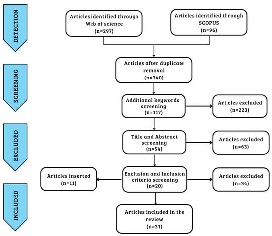
Figure 1. Prism diagram of research strategy workflow.

Table 1. Keywords, inclusion criteria, and exclusion criteria.

3.2. Analysis of Extracted Data

The characteristics of the investigated studies are summarized in Table A1, Table A2, Table A3, Table A4, Table A5 and Table A6 for all 31 included articles shown in Appendix A.

Figure 2 shows the network between the main items identified in the initial dataset of 393 items as visualized using VOSviewer Software (Version 1.6.18, Centre for Science and Technology Studies, Leiden University, Leiden, The Netherlands).

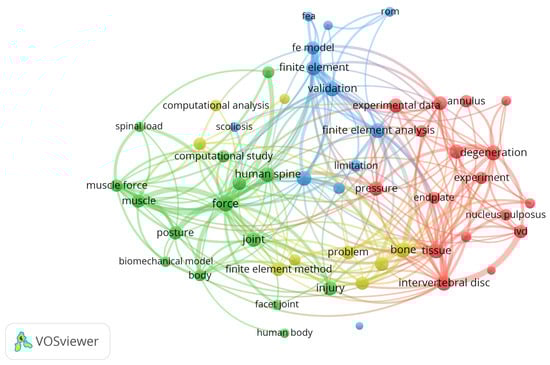
Figure 2. Network visualization for title, abstract, and keywords.

Our analysis of the network was carried out in two ways: a co-occurrence analysis, where the distance between each pair of items is calculated based on the number of documents in which the pair appears together, and a bibliographic coupling analysis, where the closeness of each pair of items is determined by the number of references they share.

Figure 3 shows the works from the initial dataset sorted by year.

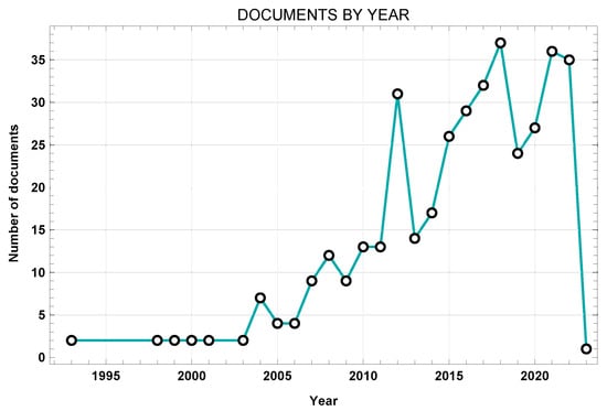
Figure 3. Network visualization of title, abstract, and keywords.

The inclusion and exclusion criteria concerned the presence of data on the modelling of the different anatomical components of the lumbar region, including the cortical bone, cancellous bone, posterior bone elements, cartilaginous endplate, annulus ground substance, annular collagen fibers, nucleus pulposus, ligaments, and follower load.

3.3. Modelling of the Different Components

Table 2 shows the most widely used modelling approaches for the anatomical components of the spine [,,,,,,,,,,,,,,,,,,,,,,,,,,,,,,].

Table 2. FE modelling and elements of the different anatomical components [,,,,,,,,,,,,,,,,,,,,,,,,,,,,,,].

3.3.1. Vertebral Body

Cancellous and cortical bone are generally modelled through linear elastic or transversely isotropic behaviour. Poroelastic modelling represents a different modelling approaches. Concerning the posterior bony elements, they are almost always modelled through linear elastic behaviour.

3.3.2. Intervertebral Disc

The nucleus pulposus can be modelled in different ways. It can be represented as an empty cavity filled with fluid, or by modelling its elastic behaviour as an incompressible material. Even if the nucleus is modelled with hyperelastic behaviour, as a rule the Neo-Hookean, Mooney–Rivlin, or Ogden model is used. Therefore, the annulus ground substance is mostly subdivided into eight or more concentric layers of fibers, starting from the outermost layer and moving to the innermost layer by varying orientation and thickness. The annular ground substance is modelled with hyperelastic behaviour using with a Neo-Hookean, Mooney–Rivlin, or Ogden model. The annular collagen fibers are modelled in terms of their nonlinear behavior or by using elastic isotropic material properties that vary with each layer.

3.3.3. Ligaments

The seven major ligaments can be treated as connector, truss, or beam elements. The constitutive models used are usually nonlinear models or isotropic elastic response models with a varying Young’s modulus according to the strain rate. Other approaches exploit non-linear

σ - ϵ

curves based on experimental data.

3.3.4. Cartilaginous Endplates and Facet Joints

The cartilaginous endplates are modelled through isotropic elastic or hyperelastic behaviour. Facet joints are often modelled through simple surface-to-surface contacts, or alternatively as uni-directional gaps or other types of contact (i.e., tie contact conditions or constraints). In addition, facet joints are modelled with a certain thickness and with isotropic or hyperelastic elastic properties.

3.4. Boundary-Loading Conditions and Validation

With respect to boundary conditions, the inferior surface of the L5 vertebra or S1 level is blocked, preventing it from moving vertically along the loading direction while being left free to rotate in other directions [,,,,,,,,,,,,,,,,,,,,,,,,,,,,,,].

Concerning the loading conditions, a compression pre-loading conditions is often applied [,,,,,,,,,,,,,,,,,,,,,,,,,,,,,,,,,]. The pre-load is usually a follower pre-load, though it can be a compressive load as well, mimicking the natural compressive load condition during upright standing. Other approaches to loading involve lateral bending and the extension or flexion moments. A downward vertical displacement setting may be used to simulate the effect of compression, and thereby the effect on intradiscal pressure. Torsion is applied as well.

The action of the muscular trunk is schematized through the follower load generated by the spine. The path for the follower load can be created as a force passing through the instantaneous centers of spinal rotation. In a different way, it can be ensured that the force path follows the curvature of the spine; the follower force may be ignored for specific applications where this does not need to be simulated.

The validation process of FE simulations generally follows the results obtained experimentally from samples of human vertebrae, though tests involving animal specimens can be a viable option as well. The experiments used for validation differ widely among different studies according to their specific testing characteristics and available in-house options. A number of experiments concern loading conditions on the spinal column based on the action of muscle forces. Other experiments involve the effects that a given loading condition has on the IDP or facet joints, while other allow for full investigate of the biomechanical response and stiffness of the seven main spinal ligaments and the collagen fibers of the intervertebral disc.

Figure 4 shows several of the principal loading conditions to which the spine is subjected.

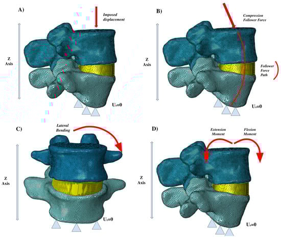
Figure 4. Different loading conditions: (A) imposed displacement, (B) compression follower force, (C) lateral bending, (D) extension and flexion moments.

4. Discussion

The present study involved a schematic literature review conducted to fully analyze the existing literature about FE modelling of the lumbar spine. This work involved number of different steps. First, a search was conducted through the Web of Science and Scopus databases in order to find the most relevant works, using specific keywords to identify the most innovative approaches. A laborious screening process followed, starting with the removal of duplicates, then further screening through additional keywords, title, and abstract. A total of 31 articles were included in the final review, each of which was exhaustively examined. The nature of the selected articles was assessed through the VosViewer software. Figure 2 demonstrates how most current investigations have focused on topics aligned with the database research concerning the following: the lumbar spine, FE analysis, computational analysis, spinal load, validation, etc. Network visualization was essential for verifying the relevance of the resulting database. It can be clearly seen that the obtained database suits the desired search parameters. Afterwards, the publication dates were analyzed. Figure 3 highlights the works in the source database, showing that they cover a wide temporal interval ranging from 1992 to 2022. This range allowed us to observe both the evolution and the consistency of computational modelling techniques of the lumbar spine over the years.

The final step was the extraction of data from articles presented in this review. All articles were carefully examined in order to extract the researchers’ choices in modelling the different parts of the considered anatomical area along with the numerical techniques used for the boundary conditions, loading conditions, and model validation process [,,,,,,,,,,,,,,,,,,,,,,,,,,,,,,]. All of this information is included in Table A1–Table A6. These tables show the modelling proposed by the different research groups, as well as their approaches to FE. The information was extracted separately in relation to the cortical bone, cancellous bone, posterior bone elements, cartilaginous endplates, annulus ground substance, annular collagen fibers, nucleus pulposus, ligaments, and follower load. Based on a careful analysis and data extraction process, the main models used by researchers were stratified and presented; see Table 2.

Cortical bone and cancellous bone are the anatomical components that exhibit the most similar numerical approaches. Isotropic elastic modelling represents a good assumption, though modelling with transverse behaviour would be the best choice to simulate the unique characteristics of cortical bone and the trabecular architecture. Posterior bone segments can be schematized simply through linear elastic behavior, and is used by most researchers. The cartilaginous endplates can be schematized by linear elastic behavior or even as a hyperelastic Neo-Hookean material. The computational results obtained from Von Mises stress analysis or from verification of the component displacement allows for a certain homogeneity in the literature to be observed from the data obtained from simulations in relation to these models.

The intervertebral disc is the most challenging to model because of its three different components, i.e., the nucleus pulposus, annular ground substance, and annular collagen fibers. Overall, the disc exhibits viscoelastic behaviour, which means that hyperelastic modelling is the most appropriate. Many different hyperelastic models are used for the annular ground substance and the nucleus pulposus; among the most common are the Mooney–Rivlin and Neo-Hookean models. Other hyperelastic models are used as well, though the Mooney–Rivlin and Neo-Hookean aprroach are both effective in capturing the biomechanical disc response. Concerning the modeling of the annulus collagen fibers, they can be modelled in a number of different ways. Because these fibers provide important mechanical strength to the annulus, the most appropriate modelling approach is the isotropic linear elastic material model. Nonlinear material behaviour has been used as well. The final results of the computational simulations show that, when using the same modelling, the results of Von Mises stresses, displacements, and intradiscal pressure analysis are quite similar to each other. Different results can be observed depending on the constitutive model chosen for modelling based on whether more or less account is taken of the elasticity or viscoelasticity of the component, whether possible damage to the disc is considered, and other situations.

All seven spinal ligaments must be modeled, as they are essential in stabilizing the spine. The most common modelling approach is a linear elastic approach using different Young’s moduli as the strain rate changes. Modelling based on nonlinear behavior can be used as well, although the lack of experimental data poses challenges when using this approach. The literature presents a number of different approaches to modelling of the facet joints. Several studies suggest using hyperelastic behavior, while others use simple surface-to-surface contact or unidirectional gap contact.

For loading conditions, Figure 4 shows the main loading conditions of the vertebral segments. The follower force is among the most important, and is often schematized by researchers based on the realization that one path line passes through all the rotational centers of the vertebrae. Lastly, the loading conditions of lateral bending, flexion, extension, and axial rotation are common to almost all of the studies we investigated. The validation process generally uses results obtained experimentally on samples of human vertebrae, although tests involving animal specimens can be a viable option. It is crucial to have the opportunity to computationally simulate the biomechanical behaviour of the spine because of the practical and economic difficulties in performing in vivo experiments. One important tool is statistical shape modelling (SSM), which is used to generate a 3D atlas of the spine that can be deformed based on specific boundaries to develop new anatomic models []. Among the different approaches used for validation [,,,,,,,,,,,], Wilke et al. [] performed an experiment on human vertebrae and then simulated and verified the effect of the muscular forces on spinal loading. This was done in order to understand how the muscular loading impacted intradiscal pressure by pure flexion and extension, lateral bending, and lateral rotation tests. Yamamoto et al. [] implemented ad hoc experimental tests to investigate the stresses incurred by the facet joints during normal bending and extension loading conditions. Meanwhile, other researchers [] have pursued validation concerning the collagen fibers of the annular ground substance to better explain the stiffness and response of the fibers under different loading conditions. Several different experimental approaches have been used to verify the biomechanical response of the spine considering the response of the ligaments, disc, and facet joints [,,].

Based on our literature review, general guidelines to modeling the lumbar vertebral body can be identified to improve the current scientific literature. Cortical and cancellous bone should be schematized through transversely elastic behavior in order to underline their true mechanical responses. Posterior bone segments can either follow the same modeling as cortical and cancellous bone or be schematized through linear isotropic elastic behavior. Modelling realised in this way guarantees the truthful modelling of the biomechanical behaviour of the components. The intervertebral disc is the component most likely to vary in modelling, depending on whether or not all components are present. The disc should be correctly schematized as the annulus ground substance, annular collagen fibers, and nucleus pulposus in order to properly simulate its biomechanics. Mooney–Rivlin hyperelastic modeling works quite well for the nucleus pulposus and annular ground substance, though future investigations might consider using different constitutive behaviours to considering the viscoelastic creep characteristics of the disc, as suggested by Sciortino [], as well as its poroelastic behavior. For future studies, the intervertebral disc could be modelled through a poroelastic model, considering that its precisely biphasic nature is guaranteed by the presence of the “liquid” part of the nucleus pulposus and the “solid” part of the fibrous ring. Concerning spinal ligaments, all studies proceed with modeling in a similar way using elastic or nonlinear behaviour. However, there is variability in the results of simulations depending on the ligament modelling choices. Viscoelastic models have not yet been widely used in the literature to simulate the mechanical response of the ligaments, e.g., the use of combined springpot, spring, and dashpot models to simulate their viscoelastic nature, even though this has already been sufficiently demonstrated in the literature. Thus, future modeling might investigate better constitutive modelling approach to account for these viscoelastic characteristics. Considering the intrinsically viscoelastic nature of these biological tissues when modelling the spinal column could ensure the accurately simulation of the the kinematics, dynamics, and static behaviour of the spine. It should be noted that the present study does have a number of limitations. First, the choice of keywords, although reasoned, could represent a limitation on the selection of the articles. Changing a keyword distorts the search results in the database by including more or fewer articles. A further limitation concerns the data extracted from the articles. Data were extracted only from those articles that presented all modelled anatomical components of interest. Those articles without a clear description of anatomy modelling methods were excluded. By excluding articles with an absence of data, the screening process certainly eliminated articles with a valid invoice. Future studies might consider adding more databases and decreasing the number of keywords in order to obtain a more detailed and comprehensive database.

5. Conclusions

This study consolidates the existing knowledge and methodologies pertaining to finite element modeling of the lumbar spinal column. The literature shows that there is a wide range of different methodologies available to schematize the lumbar spine. The result achieved by this review was to provide an overview of the different methodologies, and then combine them into a general framework based on which seem most appropriate for obtaining a well-established, reliable, and truthful FEM model. The outcome achieved by this review enables us to lay the groundwork for future research on FEM modelling of the lumbar spine, which can be realized using the notions learned and shared through this review work. Comparative insight into the different methods used is helpful in creating guidelines for future research in this field. Furthermore, it should be noted that the differences between the methodologies observed in this review is a result of different resources, research purposes, and desired levels of accuracy in the analysed studies. Future research should be based on the results extracted from the literature, including consideration of the viscoelastic characteristics of the disc and ligaments that are not fully involved in modeling. Therefore, the goal of our future work will be to precisely implement new methodologies that consider these aspects, which remain neglected today.

Author Contributions

Conceptualization, V.S. and D.C.; methodology, V.S. and S.P.; software, V.S.; formal analysis, V.S.; writing—original draft preparation, V.S., S.P., T.I. and D.C.; writing—review and editing, V.S., S.P., T.I. and D.C.; supervision, D.C. All authors have read and agreed to the published version of the manuscript.

Funding

This research received no external funding.

Institutional Review Board Statement

Not applicable.

Informed Consent Statement

Informed consent was obtained from all subjects involved in the study.

Data Availability Statement

The data presented in this study are available on request from the corresponding author. The data are not publicly available for to ethical reasons.

Conflicts of Interest

The authors declare no conflict of interest.

Appendix A

Table A1, Table A2, Table A3, Table A4, Table A5 and Table A6, shown below, were created from information extracted from the articles included in the review about the constitutive model and element type used for the modelling of the cortical bone, cancellous bone, posterior bony elements, cartilaginous endplates, annular ground substance, annular collagen fibers, nucleus pulposus, ligaments, facet joints, and follower force.

Table A1. The main information extracted from [,,,,].

	Chen et al. (2001) []			Schimdt et al. (2006) []			Chen et al. (2008) []			Rohlmann et al. (2009) []			Zander et. al. (2009) []
Anatomical Component	Constitutive Model		Element Type	Constitutive Model		Element Type	Constitutive Model		Element Type	Constitutive Model		Element Type	Constitutive Model		Element Type
Cortical Bone	Isotropic Elastic E = 12,000 MPa $ν$ = 0.3		8-node Solid	Transversely Isotropic $E_{x x}$ = 11300 MPa $ν_{x y}$ = 0.484 $E_{y y}$ = 11,300 MPa $ν_{x z}$ = 0.203 $E_{z z}$ = 22,000 MPa $G_{x y}$ = 3800 MPa $G_{y z}$ = 5400 MPa $G_{x z}$ = 5400 MPa		8-node Solid	Transversely Isotropic $E_{x x}$ = 11,300 MPa $ν_{x y} = 0.484$ $E_{y y}$ = 11,300 MPa $ν_{x z}$ = 0.203 $E_{z z}$ = 22,000 MPa $G_{x y}$ = 3800 MPa $G_{y z}$ = 5400 MPa $G_{x z}$ = 5400 MPa		8-node Solid	Isotropic Elastic E = 10,000 MPa $ν$ = 0.3		8-node Solid	Isotropic Elastic E = 10,000 MPa $ν$ = 0.3		8-node Solid
Cancellous Bone	Isotropic Elastic E = 100 MPa $ν$ = 0.2		8-node Solid	Transversely Isotropic $E_{x x}$ = 140 MPa $ν_{x y}$ = 0.450 $E_{y y}$ = 140 MPa $ν_{y z}$ = 0.315 $E_{z z}$ = 200 MPa $ν_{x z}$ = 0.325 $G_{x y}$ = 48.3 MPa $G_{y z}$ = 48.3 MPa $G_{x z}$ = 48.3 MPa		8-node Solid	Transversely Isotropic $E_{x x}$ = 140 MPa $ν_{x y}$ = 0.450 $E_{y y}$ = 140 MPa $ν = 0.315$ $E_{z z}$ = 200 MPa $ν = 0.315$ $G_{x y}$ = 48.3 MPa $G_{y z}$ = 48.3 MPa $G_{x z}$ = 48.3 MPa		8-node Solid	Transversely Isotropic $E_{x x}$ = 140 MPa $ν_{x y}$ = 0.450 $E_{y y}$ = 140 MPa $ν_{y z} = 0.315$ $E_{z z}$ = 200 MPa $ν_{x z} = 0.315$		8-node Solid	Transversely Isotropic $E_{x x}$ = 140 MPa $E_{y y}$ = 140 MPa $E_{z z}$ = 200 MPa $ν_{x z} = 0.315$		8-node Solid
Posterior bone elements	Isotropic Elastic E = 3500 MPa $ν$ = 0.25		8-node Solid	Isotropic Elastic E = 3500 MPa $ν$ = 0.25		8-node Solid	Isotropic Elastic E = 3500 MPa $ν$ = 0.25		8-node Solid	Isotropic Elastic E = 3200 MPa $ν$ = 0.25		8-node Solid	Isotropic Elastic E = 3500 MPa $ν$ = 0.25		8-node Solid
Cartilaginous Endplate	-		-	Isotropic Elastic E = 23.8 MPa $ν$ = 0.4		8-node Solid	Isotropic Elastic E = 24 MPa $ν$ = 0.4		8-node Solid	Neo-Hokean $c_{1}$ = 0.3448, $d_{1}$ = 0.3		8/6-node Solid		Neo-Hokean $c_{1}$ = 0.3448, $d_{1}$ = 0.3	8-node Solid
Annular ground substance	Isotropic Elastic E = 4.2MPa $ν$ = 0.45		8-node Solid	Mooney-Rivlin $c_{1}$ = 0.18, $c_{2}$ = 0.045 Neo-Hookean c = 0.348, d = 0.3		8-node Solid	Mooney-Rivlin $c_{1}$ = 0.42 $c_{2}$ = 0.105		8-node Link	Neo-Hookean c = 0.3448, d = 0.3		8-node Solid	Neo-Hookean c = 0.3448, d = 0.3		8-node Solid
Annular Collagen fibers	Isotropic Elastic E = 175 MPa A = 0.76 mm $^{2}$		2-node Cable	Calibrated $σ - ε$ Non-Calibrated $σ - ε$		Spring Elements	Isotropic Elastic E = 550–357.5 MPa A = 0.76–0.35 mm $^{2}$ Change by layer		2-node Link	Non-linear and dependent on the distance from the disc centre		Spring Element	Non Linear		2-node Link
Nucleus polposus	Isotropic Elastic E = 1 MPa $ν$ = 0.499		8-node Solid	Mooney-Rivlin $c_{1}$ = 0.12, $c_{2}$ = 0.03 Isotropic Elastic E = 0.2 MPa, $ν$ = 0.4999		-	Incompressible Fluid E = 1666.7 MPa		8-node Fluid	Incompressible Fluid		Fluid Element	Incompressible Fluid		Fluid Element
Ligaments ALL PLL LF TL CL IL SL	E(MPa) 7.8–20 ( $ε ≶$ 12%) 10–20 ( $ε ≶$ 11%) 15–19.5 ( $ε ≶$ 6.2%) 10–58.7 ( $ε ≶$ 18%) 7.5–32.9 ( $ε ≶$ 25%) 10–11.6 ( $ε ≶$ 14%) 8–15 ( $ε ≶$ 20%)	A (mm $^{2}$ ) 63.7 20.0 40.0 1.8 30.0 40.0 30.0	Calibrated Force–Deflection curves Non-Calibrated Force-Deflection curves		Spring Elements		E (MPa) 7.8 10 15 10 8 10 8	A (mm $^{2}$ ) 24 14.4 40.0 3.6 30.0 26 23	2-node Link		Non Linear	Spring Elements	Non Linear		2-node Solid
Facet Joint	-		-	Contact Frictionless		-	Sliding Contact		8-node Contact	Soft Contact		-	Soft Contact		-
Follower force	-		-	-		-	-		-	Acting in the centre of each vertebral body		-	Acting in the centre of each vertebral body		-

Table A2. The main information extracted from [,,,,].

	Zander et al. (2009) []		Ayturk et al. (2010) []		Manek et al. (2012) []		Weisse et al. (2012) []			Kiapour et al. (2012) []
Anatomical Component	Constitutive Model	Element Type	Constitutive Model	Element Type	Constitutive Model	Element Type	Constitutive Model		Element Type	Constitutive Model		Element Type
Cortical Bone	Isotropic Elastic E = 10,000 MPa $ν$ = 0.3	8-node Solid	Transversely Isotropic $E_{11}$ = 8000 MPa, $ν_{12}$ = 0.4 $E_{22}$ = 8000 MPa, $ν_{13}$ = 0.35 $E_{33}$ = 12,000 MPa, $ν_{23}$ = 0.3	8-node Solid	Isotropic Elastic E = 16,000 MPa $ν$ = 0.25	Shell Element	Isotropic Elastic E depending on $ρ_{C T_{s c a n}}$ $ν$ = 0.3		8-node Solid	Isotropic Elastic E = 12,000 MPa $ν$ = 0.3		8-node Solid
Cancellous Bone	Transversely Isotropic $E_{1}$ = 200 MPa, $ν_{1}$ = 0.45 $E_{2}$ = 140 MPa, $ν_{2}$ = 0.315	8-node Solid	Based on CT scans	8-node Solid	Isotropic Elastic E = 120 MPa $ν$ = 0.25	8-node Solid	E depending on $ρ_{C T_{s c a n}}$ $ν$ = 0.3		8-node Solid	Isotropic Elastic E = 100 MPa $ν$ = 0.2		8-node Solid
Posterior bone elements	Isotropic Elastic E = 3500 MPa $ν$ = 0.25	8-node Solid	Isotropic Elastic E = 3500 MPa $ν$ = 0.3	8-node Solid	-	8-node Solid	-		-	Cortical Bone E = 12,000 MPa, $ν$ = 0.3 Cancellous Bone E = 100 MPa, $ν$ = 0.2		8-node Solid
Cartilaginous Endplate	Neo-Hookean $c_{10}$ = 0.3448, $d_{1}$ = 0.43	-	Isotropic Elastic E = 23.8 MPa, $ν$ = 0.4	8-node Solid	Isotropic Elastic E = 500 MPa, $ν$ = 0.25	8-node Solid	Neo-Hokean $c_{1}$ = 0.3448, $d_{1}$ = 0.3		8-node Solid	-		-
Annular ground substance	Neo-Hookean $c_{10}$ = 0.3448, $d_{1}$ = 0.3	8-node Solid	Fiber reinforced Yeoh material $c_{10}$ = 0.0146, $c_{20}$ = −0.0189 $c_{30}$ = 0.041 $a_{3}$ = 0.03, $b_{3}$ = 120.00	8-node Solid	Two Ring Layer Isotropic Elastic $E_{1}$ = 30 MPa, $ν_{1}$ = 0.37 $E_{2}$ = 18 MPa, $ν_{2}$ = 0.41	8-node Link	Ogden Different values		8-node Solid	Neo-Hookean $c_{10}$ = 0.3448, $d_{1}$ = 0.3		8-node Solid
Annular Collagen fibers	Non-Linear dependent on the distance from the disc centre	Rebar	-	-	-	-	Force–displacement curve		8-node Solid	Isotropic Elastic E = 357–550 MPa, $ν$ = 0.3		Rebar
Nucleus polposus	Incompressible	Fluid	Isotropic Elastic, E = 1 MPa $ν$ = 0.499	-	Isotropic Elastic E = 2 MPa, $ν$ = 0.499	8-node Fluid	Mooney Rivlin $c_{1}$ = 0.12, $c_{2}$ = 0.03		8-node Solid	Incompressible Fluid E = 1 MPa, $ν$ = 0.499		Fluid Element
Ligaments ALL PLL LF TL CL IL SL	Non Linear	Spring Elements	Exponential force displacement curves	Spring Elements	-	-		Force displacement curve	Spring Elements	E (MPa) 7.8–20 ( $ε ≶$ 12%) 10-20 ( $ε ≶$ 11%) 15–19.5 ( $ε ≶$ 6.2%) 10–58.7 ( $ε ≶$ 18%) 7.5–32.9 ( $ε ≶$ 25%) 10–11.6 ( $ε ≶$ 14%) 8–15 ( $ε ≶$ 20%)	$ν$ 0.3 0.3 0.3 0.3 0.3 0.3 -	Truss Elements
Facet Joint	Soft Contact	-	Neo-Hokean $c_{10}$ = 2	-	Isotropic Elastic E = 2.28 MPa, $ν$ = 0.3	8-node Solid	Isotropic Elastic E = 24 MPa, $ν$ = 0.45		Surface to surface	Unidirectional Gap		-
Followerv force	Acting in the centre of each vertebral body	-	-	-	-	-	Acting in the centre of each vertebral body		-	Acting in the centre of each vertebral body		-

Table A3. The main information extracted from [,,,,].

	Little et al. (2013) []		Schmidt et al. (2013) []		Park et al. (2013) []		Kim et al. (2015) []			Erbulut et al. (2015) []
Anatomical Component	Constitutive Model	Element Type	Constitutive Model	Element Type	Constitutive model	Element Type	Constitutive Model		Element Type	Constitutive Model		Element Type
Cortical Bone	Isotropic Elastic E = 113,000 MPa $ν$ = 0.2	4-node Shell	Poroelastic Model E = 10,000 MPa $ν$ = 0.3 Poroelastic coefficients	-	Isotropic Elastic E = 12,000 MPa, $ν$ = 0.3	Solid Element	Transversely Isotropic $E_{x x}$ = 11,300 MPa, $ν_{x y}$ = 0.484 $E_{y y}$ = 11,300 MPa, $ν_{x z}$ = 0.203 $E_{z z}$ = 22,000 MPa $G_{x y}$ = 3800 MPa $G_{y z}$ = 5400 MPa $G_{x z}$ = 5400 MPa		-	Isotropic Elastic E = 12,000 MPa $ν$ = 0.3		Solid
Cancellous Bone	Isotropic Elastic E = 140 MPa $ν$ = 0.2	First-Order Break	Poroelastic Model E = 100 MPa $ν$ = 0.2 Poroelastic coefficients	-	Isotropic Elastic E = 190 MPa $ν$ = 0.2	Solid Element	Transversely Isotropic $E_{x x}$ = 140 MPa, $ν_{x y}$ = 0.450 $E_{y y}$ = 140 MPa, $ν_{x z}$ = 0.315 $E_{z z}$ = 200 MPa $G_{x y}$ = 48.3 MPa $G_{y z}$ = 48.3 MPa $G_{x z}$ = 48.3 MPa		-	Isotropic Elastic E = 450 MPa $ν$ = 0.25		Solid
Posterior bone elements	Quasi-Rigid	Linear Beam	-	-	Isotropic Elastic E = 35,000 MPa, $ν$ = 0.25	Solid Element	Isotropic Elastic E = 3500 MPa, $ν$ = 0.25		-	Isotropic Elastic E = 3500 MPa, $ν$ = 0.25		Solid
Cartilaginous Endplate	-	-	Poroelastic Model E = 10,000 MPa, $ν$ = 0.3 Other coefficients	-	Isotropic Elastic E = 23.8 MPa, $ν$ = 0.4	Solid Element	Isotropic Elastic E = 24 MPa, $ν$ = 0.4		-	Modelled		-
Annular ground substance	Mooney-Rivlin $c_{10}$ = 0.7, $c_{01}$ = 0.2	First-Order Brick	Fiber reinforced Poroelastic Model Neo-Hookean $c_{10}$ = 1.23 MPa D = 0.688 MPa $^{- 1}$	-	Mooney-Rivlin $c_{1}$ = 0.18, $c_{2}$ = 0.045	Solid Element	Isotropic Elastic E = 4.2 MPa, $ν$ = 0.4		-	Neo-Hookean $c_{10}$ = 0.3448, $D_{1}$ = 0.3		Solid
Annular Collagen fibers	Isotropic Elastic E = 500 MPa, $ν$ = 0.3	Rebar	Rebar applied to Ground Substance	-	Hyperelastic Strain rate dependent	Truss	Isotropic Elastic E = 358-550 MPa, $ν$ = 0.3		-	Isotropic Elastic E = 357–550 MPa, $ν$ = 0.3		Rebar
Nucleus polposus	Hydrostatic fluid Incompressible	4-node Fluid	Poroelastic Model Neo-Hookean $c_{10}$ = 0.627 MPa, D = 2.475 MPa $^{- 1}$	-	Different value E	Fluid Element	Isotropic Elastic E = 1 MPa, $ν$ = 0.499		-	Isotropic Elastic E = 9 MPa, $ν$ = 0.499		Solid
Ligaments ALL PLL LF TL CL IL SL	Non Linear	Connector and Spring Elements	Modelled	-	Hyperelastic Material Strain rate dependent	Truss	E (MPa) 7.8–20 ( $ε ≶$ 12%) 10–20 ( $ε ≶$ 11%) 15–19.5 ( $ε ≶$ 6.2%) 10–58.7 ( $ε ≶$ 18%) 7.5–32.9 ( $ε ≶$ 25%) 10–11.6 ( $ε ≶$ 14%) 8–15 ( $ε ≶$ 20%)	A (mm $^{2}$ ) 63.7 20.0 40.0 1.8 30.0 40.0 30.0	-	E (MPa) 7.8–20 ( $ε ≶$ 12%) 10–20 ( $ε ≶$ 11%) 15–19.5 ( $ε ≶$ 6.2%) 10–58.7 ( $ε ≶$ 18%) 7.5–32.9 ( $ε ≶$ 25%) 10–11.6 ( $ε ≶$ 14%) 8–15 ( $ε ≶$ 20%)	$ν$ 0.3 0.3 0.3 0.3 0.3 0.3 -	Truss Elements
Facet Joint	-	-	Surface to Surface Frictionless	-	Surface to Surface Soft contact	-	Surface to Surface Frictionless		-	Gap contact		-
Follower force	-	-	Acting in the centre of each vertebral body	-	Acting in the centre of each vertebral body	-	Acting in the centre of each vertebral body		-	Acting in the centre of each vertebral body		-

Table A4. The main information extracted from [,,,,].

	Barthelemy et al. (2015) []		Xu et al. (2016) []		Zander et al. (2016) []		Kang et al. (2017) []				Fan et al. (2017) []
Anatomical Component	Constitutive Model	Element Type	Constitutive Model	Element Type	Constitutive Model	Element Type	Constitutive Model			Element Type	Constitutive Model			Element Type
Cortical Bone	Isotropic Elastic E = 12,000 MPa $ν$ = 0.4	-	Isotropic Elastic E = 12,000 MPa, $ν$ = 0.3	8-node Solid	Isotropic Elastic E = 10,000 MPa	Shell Element	Transversely Elastic $E_{x x}$ = 11,300 MPa, $ν_{x y}$ = 0.484 $E_{y y}$ = 11,300 MPa, $ν_{x z}$ = 0.203 $E_{z z}$ = 22,000 MPa $G_{x}$ = 3800 MPa $G_{y}$ = 5400 MPa $G_{z}$ = 5400 MPa			Solid	Isotropic Elastic E = 12,000 MPa $ν$ = 0.3			3-node Solid
Cancellous Bone	Isotropic Elastic E = 140 MPa, $ν$ = 0.45	-	Isotropic Elastic E = 100 MPa, $ν$ = 0.20	8-node Solid	Transversely Elastic E = 100–300 MPa	-	Transversely Elastic $E_{x x}$ = 140 MPa, $ν_{x y}$ = 0.45 $E_{y y}$ = 140 MPa, $ν_{x z}$ = 0.315 $E_{z z}$ = 200 MPa $G_{x}$ = 48.3 MPa $G_{y}$ = 48.3 MPa $G_{z}$ = 48.3 MPa			4-node Solid	Isotropic Elastic E = 100 MPa, $ν$ = 0.2			4-node Solid
Posterior bone elements	Isotropic Elastic E = 35,000 MPa, $ν$ = 0.30	-	Isotropic Elastic E = 35,000 MPa, $ν$ = 0.25	8-node Solid	Isotropic Elastic E = 35,000 MPa	-	Isotropic Elastic E = 3500 MPa, $ν$ = 0.25			4-node Solid	Isotropic Elastic E = 3500 MPa, $ν$ = 0.25			4-node Solid
Cartilaginous Endplate	Isotropic Elastic E = 1000 MPa, $ν$ = 0.30	-	Isotropic Elastic E = 23.89 MPa, $ν$ = 0.40	8-node Solid	-	-	Isotropic Elastic E = 23.89 MPa, $ν$ = 0.40			Solid	Isotropic Elastic E = 23.8 MPa, $ν$ = 0.4			3-node Solid
Annular ground substance	Osmo-poro-viscoelastic	-	Mooney-Rivlin $c_{1}$ = 0.56, $c_{2}$ = 0.14, $ν$ = 0.45	8-node Solid	Neo-Hookean $c_{10}$ = 0.3448, $D_{1}$ = 0.3	-	Mooney-Rivlin $c_{1}$ = 0.2, $c_{2}$ = 0.05			Solid	Mooney-Rivlin $c_{10}$ = 0.18, $c_{01}$ = 0.045			8-node Solid
Annular Collagen fibers	-	-	Nonlinear $σ - ε$ curve	4-node Shell Rebar	Nonlinear $σ - ε$ curve	-	Different value E			Truss	-			-
Nucleus polposus	Osmo-poro-viscoelastic	-	Mooney-Rivlin $c_{10}$ = 0.12, $c_{01}$ = 0.09, $ν$ = 0.4999	8-node Solid	Hydrostatic	-	Isotropic Elastic E = 1 MPa, $ν$ = 0.499			8-node Solid	Mooney-Rivlin $c_{10}$ = 0.12, $c_{01}$ = 0.09, $ν$ = 0.4999			Solid
Ligaments ALL PLL LF TL CL IL SL	Hypoelastic	Truss	Non-Linear $σ - ε$ curve	4-node Shell	Non-Linear $σ - ε$ curve	-		E (MPa) 7.8–20 ( $ε ≶$ 12%) 10–20 ( $ε ≶$ 11%) 15–19.5 ( $ε ≶$ 6.2%) 10–58.7 ( $ε ≶$ 18%) 7.5–32.9 ( $ε ≶$ 25%) 10–11.6 ( $ε ≶$ 14%) 8–15 ( $ε ≶$ 20%)	$ν$ 0.3 0.3 0.3 0.3 0.3 0.3 -	Truss Elements		E (MPa) 7.8–20 ( $ε ≶$ 12%) 10–20 ( $ε ≶$ 11%) 15–19.5 ( $ε ≶$ 6.2%) 10–58.7 ( $ε ≶$ 18%) 7.5–32.9 ( $ε ≶$ 25%) 10–11.6 ( $ε ≶$ 14%) 8–15 ( $ε ≶$ 20%)	$ν$ 0.3 0.3 0.3 0.3 0.3 0.3 -	Truss Elements
Facet Joint	Surface to Surface Frictionless	-	Soft frictionless contact	-	Surface to Surface contact	-	Surface to Surface frictionless			-	Surface to Surface frictionless			-
Follower force	-	-	Acting in the centre of each vertebral body	-	-	-	Acting in the centre of each vertebral body			-	Acting in the centre of each vertebral body			-

Table A5. The main information extracted from [,,,,].

	Finley et al. (2018) []		Zhou et al. (2019) []		Fan et al. (2019) []			Mills et al. (2019) []			Haj-Ali et al. (2019) []
Anatomical Component	Constitutive Model	Element Type	Constitutive Model	Element Type	Constitutive Model		Element Type	Constitutive Model		Element Type	Constitutive Model		Element Type
Cortical Bone	Transversely Elastic $E_{1}$ = 8000 MPa $ν_{12}$ = 0.4 $E_{2}$ = 8000 MPa $ν_{23}$ = 0.3 $E_{3}$ = 12,000 MPa $ν_{31}$ = 0.35	Solid Element	Isotropic Elastic E = 12,000 MPa, $ν$ = 0.3	-	Isotropic Elastic E = 12,000 MPa, $ν$ = 0.3		Solid Element	Transversely Elastic $E_{x x}$ = 11,300 MPa, $ν_{x y}$ = 0.484 $E_{x z}$ = 11,300 MPa, $ν_{x z}$ = 0.203 $E_{z z}$ = 22,000 MPa $G_{x}$ = 3800 MPa $G_{y}$ = 5400 MPa $G_{z}$ = 5400 MPa		-	Isotropic Elastic E = 12,000 MPa $ν$ = 0.3		Solid Element
Cancellous Bone	Neo-Hookean E = 100 MPa $ν$ = 0.2	Solid Element	Transversely Elastic $E_{x x}$ = 140 MPa, $ν_{x y}$ = 0.45 $E_{y y}$ = 140 MPa, $ν_{x z}$ = 0.315 $E_{z z}$ = 200 MPa $G_{x}$ = 48.3 MPa $G_{y}$ = 48.3 MPa $G_{z}$ = 48.3 MPa	-	Isotropic Elastic E = 100 MPa $ν$ = 0.2		Solid	Transversely Elastic $E_{x x}$ = 140 MPa, $ν_{x y}$ = 0.45 $E_{y y}$ = 140 MPa, $ν_{x z}$ = 0.315 $E_{z z}$ = 200 MPa $G_{x}$ = 48.3 MPa $G_{y}$ = 48.3 MPa $G_{z}$ = 48.3 MPa		-	Isotropic Elastic E = 100 MPa, $ν$ = 0.2		Solid Element
Posterior bone elements	Neo-Hookean E = 35,000 MPa $ν$ = 0.30	-	Isotropic Elastic E = 35,000 MPa $ν$ = 0.25	-	Isotropic Elastic E = 35,000 MPa $ν$ = 0.25		-	Isotropic Elastic E = 3500 MPa, $ν$ = 0.25 G = 1400 MPa		-	-		-
Annular Collagen fibers	Exponentialpower $α$ = 65 MPa, $β$ = 2 MPa $ζ$ = 0.296 MPa	-	Annular Lamellae Non-linear	-	Isotropic Elastic E = 360–550 MPa		-	Two layers $k_{1}$ = 3 MPa, $k_{2}$ = 45 MPa		-	-		-
Cartilaginous Endplate	Neo-Hookean E = 23.8 MPa, $ν$ = 0.42	-	Isotropic Elastic E = 24 MPa, $ν$ = 0.40	-	Isotropic Elastic E = 23.8 MPa, $ν$ = 0.4		Solid	-		-	-		-
Annular ground substance	Holmes-Mow E = 1 MPa, $ν$ = 0.4 $β$ = 3.4	-	Mooney-Rivlin $c_{1}$ = 0.18, $c_{2}$ = 0.045	-	Mooney-Rivlin $c_{1}$ = 0.18, $c_{2}$ = 0.045		Solid Element	Neo-Hookean $c_{10}$ = 0.250		Solid	Isotropic Elastic E = 8.4 MPa, $ν$ = 0.45		Solid
Nucleus polposus	Neo-Hookean E = 1 MPa, $ν$ = 0.49	-	Mooney-Rivlin $c_{10}$ = 0.12, $c_{01}$ = 0.03	-	Mooney-Rivlin $c_{10}$ = 0.12, $c_{01}$ = 0.03		Solid	Mooney-Rivlin $c_{10}$ = 0.12, $c_{01}$ = 0.03		8-node Solid	Isotropic Elastic E = 1 MPa $ν$ = 0.4999		Solid
Ligaments ALL PLL LF TL CL IL SL	Non-linear	Spring Elements	Non-Linear force-deflection relation	-	E (MPa) 7.8–20 ( $ε ≶$ 12%) 10–20 ( $ε ≶$ 11%) 15–19.5 ( $ε ≶$ 6.2%) 10–58.7 ( $ε ≶$ 18%) 7.5–32.9 ( $ε ≶$ 25%) 10–11.6 ( $ε ≶$ 14%) 8–15 ( $ε ≶$ 20%)	A (mm $^{2}$ ) 63.7 20 40 1.8 30 40 30	Truss		Tension-only	-		Different modelling Non-linear E varying on $ε$ -rate	-
Facet Joint	Neo-Hookean E = MPa, $ν$ = 0.4	-	Isotropic Elastic E = 35 MPa, $ν$ = 0.4	-	-		-	Non-Linear Isotropic elastic Surface to surface		-	Contact Frictionless		-
Follower force	Acting in the centre of each vertebral body	-	Acting in the centre of each vertebral body	-	Acting in the centre of each vertebral body		-	-		-	-		-

Table A6. The main information extracted from [,,,,,].

	Affolter et al. (2020) []		Godinho et al. (2021) []				Sengul et al. (2021) []		Turbucz et al. (2022) []		Sanjay et al. (2022) []			Tan et al. (2022) []
Anatomical Component	Constitutive Model	Element Type	Constitutive Model			Element Type	Constitutive Model	Element Type	Constitutive Model	Element Type	Constitutive Model		Element Type	Constitutive Model	Element Type
Cortical Bone	Transversely Elastic	Solid Element	Isotropic Elastic E = 1200 MPa, $ν$ = 0.3			Solid	Isotropic Elastic E = 12,000 MP, $ν$ = 0.3	Shell Element	Isotropic Elastic E = 10,000 MPa, $ν$ = 0.3	Solid	Isotropic Elastic E = 12,000 MPa, $ν$ = 0.3		Solid Element	Isotropic Elastic E = 12,000 MPa, $ν$ = 0.3	Solid Element
Cancellous Bone	Transversely Elastic	Solid Element	Transversely Elastic E = 200 MPa, $ν$ = 0.315			Solid Element	Isotropic Elastic E = 100 MPa, $ν$ = 0.2	Solid	Isotropic Elastic E = 100 MPa, $ν$ = 0.2	Solid Element	Isotropic Elastic E = 100 MPa, $ν$ = 0.3		Solid Element	Isotropic Elastic E = 100 MPa, $ν$ = 0.3	Solid Element
Posterior bone elements	Transversely Elastic	Solid Element	-			-	-	-	Isotropic Elastic E = 3500 MPa, $ν$ = 0.25	Solid Element	-		-	Isotropic Elastic E = 3500 MPa, $ν$ = 0.25	Solid Element
Cartilaginous Endplate	Modelled	-	Modelled			-	Isotropic Elastic E = 23.8 MPa, $ν$ = 0.4	Solid Element	Isotropic Elastic E = 23.8 MPa, $ν$ = 0.42	Solid Element	Isotropic Elastic E = 23.8 MPa, $ν$ = 0.4		Solid	Isotropic Elastic E = 24 MPa	Solid
Annular ground ubstance	Hyperelastic Model	Solid Element	Holzapfel $D_{1}$ = 0.254 MPa $^{- 1}$ $k_{1}$ = 12 MPa $k_{2}$ = 300, k = 0.1			Solid	Mooney-Rivlin $c_{10}$ = 0.13 $c_{01}$ = 0.03 D = 0.6	Solid Element	Mooney-Rivlin $c_{10}$ = 0.18 $c_{01}$ = 0.045	Solid	Isotropic Elastic E = 9 MPa, $ν$ = 0.4		Solid	Mooney-Rivlin	Solid
Annular Collagen fibers	Non-Linear	Rebar	-			-	Isotropic Elastic E = 360–550 MPa $ν$ = 0.45	Rebar	Non-Linear $σ - ε$ -curve	Truss Element	-		-	Non-Linear $σ - ε$ - calibrated curve	Spring Element
Ligaments ALL PLL LF TL CL IL SL	Ogdenr 3rd Order	-		E (MPa) 20 10 13 12 7.5 9.8 8.8	A (mm $^{2}$ ) 75.9 1.6 39 1.8 19 1.8 6	-	Non-Linear	Connector	Non-Linear	Spring		E (MPa) 45.20 26.49 43.71 2.77 - 35.50 12.72	-	Tension-only	Spring
Nucleus polposus	Fluid Cavity	Fluid	Mooney-Rivlin $c_{10}$ = 0.315 $c_{01}$ = 0.03 $D_{1}$ = 0.667			-	Isotropic Elastic E = 1 MPa $ν$ = 0.499	Solid	Mooney-Rivlin $c_{10}$ = 0.12, $c_{01}$ = 0.03	8-node Solid	Isotropic Elastic E = 0.1 MPa $ν$ = 0.49		Solid	Mooney-Rivlin	-
Facet Joint	-	-	Gap contact Surface to surface			-	Gap contact	-	Neo-Hookean $c_{10}$ = 5.36, $D_{1}$ = 0.04	Solid	Gap contact		-	Neo-Hookean	Solid
Follower force	Acting in the centre of each vertebral body	-	-			-	-	-	Acting in the centre of each vertebral body	-	-		-	Acting in the centre of each vertebral body	-

References

Fung, Y.C. Biomechanics: Biomechanics Mechanical Properties of Living Tissues, 2nd ed.; Springer: New York, NY, USA, 2010. [Google Scholar]
Benzel, E.C. Deformity Prevention and Correction: Component Strategies; Biomechanics of Spine Stablization; AANS Publications: Rolling Meadows, IL, USA, 2001; pp. 437–440. [Google Scholar]
Orías, A.A.E.; He, J.; Wang, M. Biomechanical Testing of the Intact and Surgically Treated spine. In Experimental Methods in Orthopaedic Biomechanics; Academic Press: Cambridge, MA, USA, 2017; pp. 133–147. [Google Scholar]
Noailly, J.; Lacroix, D. Finite Element Modelling of the Spine. In Biomaterials for Spinal Surgery; Woodhead Publishing: Sawston, UK, 2012; pp. 144–234. [Google Scholar]
Kramer, P.A.; Hammerberg, A.G.; Sylvester, A.D. Modeling the spine using finite element models: Considerations and cautions. In Spinal Evolution; Springer: Cham, Switzerland, 2019; pp. 387–400. [Google Scholar]
Kurutz, M.; Oroszváry, L. Finite element modeling and simulation of healthy and degenerated human lumbar spine. In Finite Element Analysis—From Biomedical Applications to Industrial Developments; IntechOpen Limited: London, UK, 2012. [Google Scholar]
Martini, F.; Timmons, M.J.; Tallitsch, R.B.; Ober, W.C.; Garrison, C.W.; Welch, K.B.; Hutchings, R.T. Human Anatomy, 9th ed.; Prentice Hall: Hoboken, NJ, USA, 2017; p. 904. [Google Scholar]
Lu, Y.M.; Hutton, W.C.; Gharpuray, V.M. The Effect of Fluid Loss on the Viscoelastic Behavior of the Lumbar Intrevertebral Disc in Compression. J. Biomech. Eng. 1998, 120, 48–54. [Google Scholar] [CrossRef] [PubMed]
Patwardhan, A.G.; Havey, R.M.; Meade, K.P.; Lee, B.; Dunlap, B. A follower load increases the load-carrying capacity of the lumbar spine in compression. Spine 1999, 24, 1003–1009. [Google Scholar] [CrossRef]
Kim, Y.H.; Kim, K. Computational modeling of spine and trunk muscles subjected to follower force. J. Mech. Sci. Technol. 2007, 21, 568–574. [Google Scholar] [CrossRef]
Kim, K.; Kim, Y.H. Role of trunk muscles in generating follower load in the lumbar spine of neutral standing posture. J. Biomech. Eng. 2008, 130, 041005. [Google Scholar] [CrossRef] [PubMed]
Han, K.S.; Rohlmann, A.; Yang, S.J.; Kim, B.S.; Lim, T.H. Spinal muscles can create compressive follower loads in the lumbar spine in a neutral standing posture. Med. Eng. Phys. 2011, 33, 472–478. [Google Scholar] [CrossRef]
Dreischarf, M.; Zander, T.; Shirazi-Adl, A.; Puttlitz, C.M.; Adam, C.J.; Chen, C.S.; Goel, V.K.; Kiapour, A.; Kim, Y.H.; Labus, K.M.; et al. Comparison of eight published static finite element models of the intact lumbar spine: Predictive power of models improves when combined together. J. Biomech. 2014, 47, 1757–1766. [Google Scholar] [CrossRef] [PubMed]
Ayturk, U.M.; Puttlitz, C.M. Parametric convergence sensitivity and validation of a finite element model of the human lumbar spine. Comput. Methods Biomech. Biomed. Eng. 2011, 14, 695–705. [Google Scholar] [CrossRef]
Kiapour, A.; Ambati, D.; Hoy, R.W.; Goel, V.K. Effect of graded facetectomy on biomechanics of Dynesys dynamic stabilization system. Spine 2012, 37, E581–E589. [Google Scholar] [CrossRef]
Little, J.P.; De Visser, H.; Pearcy, M.J.; Adam, C.J. Are coupled rotations in the lumbar spine largely due to the osseo-ligamentous anatomy?–A modelling study. Comput. Methods Biomech. Biomed. Eng. 2008, 11, 95–103. [Google Scholar] [CrossRef]
Liu, C.L.; Zhong, Z.C.; Hsu, H.W.; Shih, S.L.; Wang, S.T.; Hung, C.; Chen, C.S. Effect of the cord pretension of the Dynesys dynamic stabilisation system on the biomechanics of the lumbar spine: A finite element analysis. Eur. Spine J. 2011, 20, 1850–1858. [Google Scholar] [CrossRef]
Park, W.M.; Kim, K.; Kim, Y.H. Effects of degenerated intervertebral discs on intersegmental rotations, intradiscal pressures, and facet joint forces of the whole lumbar spine. Comput. Biol. Med. 2013, 43, 1234–1240. [Google Scholar] [CrossRef] [PubMed]
Schmidt, H.; Galbusera, F.; Rohlmann, A.; Zander, T.; Wilke, H.J. Effect of multilevel lumbar disc arthroplasty on spine kinematics and facet joint loads in flexion and extension: A finite element analysis. Eur. Spine J. 2012, 21, 663–674. [Google Scholar] [CrossRef] [PubMed]
Shirazi-Adl, A. Biomechanics of the lumbar spine in sagittal/lateral moments. Spine 1994, 19, 2407–2414. [Google Scholar] [CrossRef] [PubMed]
Zander, T.; Rohlmann, A.; Bergmann, G. Influence of different artificial disc kinematics on spine biomechanics. Clin. Biomech. 2009, 24, 135–142. [Google Scholar] [CrossRef] [PubMed]
Wei, H.W.; Chuang, S.M.; Chen, C.S. Biomechanical Evaluation of the Lumbar Spine by Using a New Interspinous Process Device: A Finite Element Analysis. Appl. Sci. 2021, 11, 10486. [Google Scholar] [CrossRef]
Guan, Y.; Yoganandan, N.; Zhang, J.; Pintar, F.A.; Cusick, J.F.; Wolfla, C.E.; Maiman, D.J. Validation of a clinical finite element model of the human lumbosacral spine. Med. Biol. Eng. Comput. 2006, 44, 633–641. [Google Scholar] [CrossRef]
Tan, Q.C.; Huang, J.F.; Bai, H.; Liu, Z.X.; Huang, X.Y.; Zhao, X.; Yang, Z.; Du, C.-F.; Lei, W.; Wu, Z.X. Effects of Revision Rod Position on Spinal Construct Stability in Lumbar Revision Surgery: A Finite Element Study. Front. Bioeng. Biotechnol. 2021, 9, 799727. [Google Scholar] [CrossRef]
Schmidt, H.; Heuer, F.; Simon, U.; Kettler, A.; Rohlmann, A.; Claes, L.; Wilke, H.J. Application of a new calibration method for a three-dimensional finite element model of a human lumbar annulus fibrosus. Clin. Biomech. 2006, 21, 337–344. [Google Scholar] [CrossRef]
Keller, T.S.; Spengler, D.M.; Hansson, T.H. Mechanical behavior of the human lumbar spine. I. Creep analysis during static compressive loading. J. Orthop. Res. 1987, 5, 467–478. [Google Scholar] [CrossRef]
Neumann, P.; Keller, T.S.; Ekström, L.; Perry, L.; Hansson, T.H.; Spengler, D.M. Mechanical properties of the human lumbar anterior longitudinal ligament. J. Biomech. 1992, 25, 1185–1194. [Google Scholar] [CrossRef]
Patwardhan, A.G.; Havey, R.M.; Carandang, G.; Simonds, J.; Voronov, L.I.; Ghanayem, A.J.; Meade, K.P.; Gavin, T.M.; Paxinos, O. Effect of compressive follower preload on the flexion–extension response of the human lumbar spine. J. Orthop. Res. 2003, 21, 540–546. [Google Scholar] [CrossRef]
Popovich, J.M., Jr.; Welcher, J.B.; Hedman, T.P.; Tawackoli, W.; Anand, N.; Chen, T.C.; Kulig, K. Lumbar facet joint and intervertebral disc loading during simulated pelvic obliquity. Spine J. 2013, 13, 1581–1589. [Google Scholar] [CrossRef] [PubMed]
Wilke, H.J.; Wolf, S.; Claes, L.E.; Arand, M.; Wiesend, A. Influence of varying muscle forces on lumbar intradiscal pressure: An in vitro study. J. Biomech. 1996, 29, 549–555. [Google Scholar] [CrossRef] [PubMed]
Damm, N.; Rockenfeller, R.; Gruber, K. Lumbar spinal ligament characteristics extracted from stepwise reduction experiments allow for preciser modeling than literature data. Biomech. Model. Mechanobiol. 2020, 19, 893–910. [Google Scholar] [CrossRef]
Yahia, L.H.; Audet, J.; Drouin, G. Rheological properties of the human lumbar spine ligaments. J. Biomed. Eng. 1991, 13, 399–406. [Google Scholar] [CrossRef] [PubMed]
Brinckmann, P.; Grootenboer, H. Change of disc height, radial disc bulge, and intradiscal pressure from discectomy an in vitro investigation on human lumbar discs. Spine 1991, 16, 641–646. [Google Scholar] [CrossRef]
Yamamoto, I.S.A.O.; Panjabi, M.M.; Crisco, T.R.E.Y.; Oxland, T.O.M. Three-dimensional movements of the whole lumbar spine and lumbosacral joint. Spine 1989, 14, 1256–1260. [Google Scholar] [CrossRef]
Alawneh, O.; Zhong, X.; Faieghi, R.; Xi, F. Finite Element Methods for Modeling the Pressure Distribution in Human Body–Seat Interactions: A Systematic Review. Appl. Sci. 2022, 12, 6160. [Google Scholar] [CrossRef]
Chen, C.S.; Cheng, C.K.; Liu, C.L.; Lo, W.H. Stress analysis of the disc adjacent to interbody fusion in lumbar spine. Med. Eng. Phys. 2001, 23, 485–493. [Google Scholar] [CrossRef]
Schmidt, H.; Heuer, F.; Drumm, J.; Klezl, Z.; Claes, L.; Wilke, H.J. Application of a calibration method provides more realistic results for a finite element model of a lumbar spinal segment. Clin. Biomech. 2007, 22, 377–384. [Google Scholar] [CrossRef]
Zhong, Z.C.; Chen, S.H.; Hung, C.H. Load-and displacement-controlled finite element analyses on fusion and non-fusion spinal implants. Proc. Inst. Mech. Eng. Part J. Eng. Med. 2009, 223, 143–157. [Google Scholar] [CrossRef] [PubMed]
Rohlmann, A.; Zander, T.; Rao, M.; Bergmann, G. Applying a follower load delivers realistic results for simulating standing. J. Biomech. 2009, 42, 1520–1526. [Google Scholar] [CrossRef] [PubMed]
Zander, T.; Krishnakanth, P.; Bergmann, G.; Rohlmann, A. Diurnal variations in intervertebral disc height affect spine flexibility, intradiscal pressure and contact compressive forces in the facet joints. Comput. Methods Biomech. Biomed. Eng. 2010, 13, 551–557. [Google Scholar] [CrossRef]
Manek, F.; Marcián, P.; Florian, Z.; Valášek, J.; Ebringerová, V. Biomechanical Study of Lumbar Spinal Fixation Device. In Applied Mechanics and Materials; Trans Tech Publications Ltd.: Wollerau, Switzerland, 2012; Volume 232, pp. 142–146. [Google Scholar]
Weisse, B.; Aiyangar, A.K.; Affolter, C.; Gander, R.; Terrasi, G.P.; Ploeg, H. Determination of the translational and rotational stiffnesses of an L4–L5 functional spinal unit using a specimen-specific finite element model. J. Mech. Behav. Biomed. Mater. 2012, 13, 45–61. [Google Scholar] [CrossRef]
Little, J.P.; Adam, C.J. Geometric sensitivity of patient-specific finite element models of the spine to variability in user-selected anatomical landmarks. Comput. Methods Biomech. Biomed. Eng. 2015, 18, 676–688. [Google Scholar] [CrossRef]
Schmidt, H.; Bashkuev, M.; Dreischarf, M.; Rohlmann, A.; Duda, G.; Wilke, H.J.; Shirazi-Adl, A. Computational biomechanics of a lumbar motion segment in pure and combined shear loads. J. Biomech. 2013, 46, 2513–2521. [Google Scholar] [CrossRef]
Kim, H.J.; Kang, K.T.; Son, J.; Lee, C.K.; Chang, B.S.; Yeom, J.S. The influence of facet joint orientation and tropism on the stress at the adjacent segment after lumbar fusion surgery: A biomechanical analysis. Spine J. 2015, 15, 1841–1847. [Google Scholar] [CrossRef] [PubMed]
Erbulut, D.U.; Zafarparandeh, I.; Hassan, C.R.; Lazoglu, I.; Ozer, A.F. Determination of the biomechanical effect of an interspinous process device on implanted and adjacent lumbar spinal segments using a hybrid testing protocol: A finite-element study. J. Neurosurg. Spine 2015, 23, 200–208. [Google Scholar] [CrossRef]
Barthelemy, V.M.P.; Van Rijsbergen, M.M.; Wilson, W.; Huyghe, J.M.; Van Rietbergen, B.; Ito, K. A computational spinal motion segment model incorporating a matrix composition-based model of the intervertebral disc. J. Mech. Behav. Biomed. Mater. 2016, 54, 194–204. [Google Scholar] [CrossRef]
Xu, M.; Yang, J.; Lieberman, I.H.; Haddas, R. Lumbar spine finite element model for healthy subjects: Development and validation. Comput. Methods Biomech. Biomed. Eng. 2017, 20, 1–15. [Google Scholar] [CrossRef]
Zander, T.; Dreischarf, M.; Timm, A.K.; Baumann, W.W.; Schmidt, H. Impact of material and morphological parameters on the mechanical response of the lumbar spine–A finite element sensitivity study. J. Biomech. 2017, 53, 185–190. [Google Scholar] [CrossRef]
Kang, K.T.; Koh, Y.G.; Son, J.; Yeom, J.S.; Park, J.H.; Kim, H.J. Biomechanical evaluation of pedicle screw fixation system in spinal adjacent levels using polyetheretherketone, carbon-fiber-reinforced polyetheretherketone, and traditional titanium as rod materials. Compos. Part Eng. 2017, 130, 248–256. [Google Scholar] [CrossRef]
Fan, W.; Guo, L.X. Influence of different frequencies of axial cyclic loading on time-domain vibration response of the lumbar spine: A finite element study. Comput. Biol. Med. 2017, 86, 75–81. [Google Scholar] [CrossRef] [PubMed]
Finley, S.M.; Brodke, D.S.; Spina, N.T.; DeDen, C.A.; Ellis, B.J. FEBio finite element models of the human lumbar spine. Comput. Methods Biomech. Biomed. Eng. 2018, 21, 444–452. [Google Scholar] [CrossRef] [PubMed]
Zhou, C.; Cha, T.; Li, G. An upper bound computational model for investigation of fusion effects on adjacent segment biomechanics of the lumbar spine. Comput. Methods Biomech. Biomed. Eng. 2019, 22, 1126–1134. [Google Scholar] [CrossRef]
Fan, W.; Guo, L.X.; Zhao, D. Stress analysis of the implants in transforaminal lumbar interbody fusion under static and vibration loadings: A comparison between pedicle screw fixation system with rigid and flexible rods. J. Mater. Sci. Mater. Med. 2019, 30, 1–10. [Google Scholar] [CrossRef]
Mills, M.J.; Sarigul-Klijn, N. Validation of an in vivo medical image-based young human lumbar spine finite element model. J. Biomech. Eng. 2019, 141, 031003. [Google Scholar] [CrossRef]
Haj-Ali, R.; Wolfson, R.; Masharawi, Y. A patient specific computational biomechanical model for the entire lumbosacral spinal unit with imposed spondylolysis. Clin. Biomech. 2019, 68, 37–44. [Google Scholar] [CrossRef] [PubMed]
Affolter, C.; Kedzierska, J.; Vielma, T.; Weisse, B.; Aiyangar, A. Estimating lumbar passive stiffness behaviour from subject-specific finite element models and in vivo 6DOF kinematics. J. Biomech. 2020, 102, 109681. [Google Scholar] [CrossRef]
Godinho, M.I.; Carvalho, V.; Matos, M.T.; Fernandes, P.R.; Castro, A.P.G. Computational modeling of lumbar disc degeneration before and after spinal fusion. Clin. Biomech. 2021, 90, 105490. [Google Scholar] [CrossRef]
Sengul, E.; Ozmen, R.; Yaman, M.E.; Demir, T. Influence of posterior pedicle screw fixation at L4–L5 level on biomechanics of the lumbar spine with and without fusion: A finite element method. Biomed. Eng. Online 2021, 20, 1–19. [Google Scholar] [CrossRef] [PubMed]
Turbucz, M.; Pokorni, A.J.; Szőke, G.; Hoffer, Z.; Kiss, R.M.; Lazary, A.; Eltes, P.E. Development and Validation of Two Intact Lumbar Spine Finite Element Models for In Silico Investigations: Comparison of the Bone Modelling Approaches. Appl. Sci. 2022, 12, 10256. [Google Scholar] [CrossRef]
Sanjay, D.; Bhardwaj, J.S.; Kumar, N.; Chanda, S. Expandable pedicle screw may have better fixation than normal pedicle screw: Preclinical investigation on instrumented L4–L5 vertebrae based on various physiological movements. Med. Biol. Eng. Comput. 2022, 60, 2501–2519. [Google Scholar] [CrossRef] [PubMed]
Moramarco, V.D.; Del Palomar, A.P.; Pappalettere, C.; Doblaré, M. An accurate validation of a computational model of a human lumbosacral segment. J. Biomech. 2010, 43, 334–342. [Google Scholar] [CrossRef]
Sciortino, V.; Pasta, S.; Ingrassia, T.; Cerniglia, D. A Population-Based 3D Atlas of the Pathological Lumbar Spine Segment. Bioengineering 2022, 9, 408. [Google Scholar] [CrossRef]
Mimura, M.; Panjabi, M.M.; Oxland, T.R.; Crisco, J.J.; Yamamoto, I.; Vasavada, A. Disc degeneration affects the multidirectional flexibility of the lumbar spine. Spine 1994, 19, 1371–1380. [Google Scholar] [CrossRef]
Sciortino, V.; Cerniglia, D.; Pasta, S.; Ingrassia, T. Fractional Calculus as a New Perspective in the Viscoelastic Behaviour of the Intervertebral Disc. In European Workshop on Structural Health Monitoring; Springer: Cham, Switzerland, 2023; pp. 915–925. [Google Scholar]

Figure 1. Prism diagram of research strategy workflow.

Figure 2. Network visualization for title, abstract, and keywords.

Figure 3. Network visualization of title, abstract, and keywords.

Figure 4. Different loading conditions: (A) imposed displacement, (B) compression follower force, (C) lateral bending, (D) extension and flexion moments.

Table 1. Keywords, inclusion criteria, and exclusion criteria.

Keywords, Exclusion Criteria, and Inclusion Criteria	N° Articles
TITLE-ABS-KEY ((lumbar AND spine) AND (computational)	393
AND(modelling) AND (model))
After duplicate removal	340
TITLE-ABS-KEY ((lumbar AND spine) AND (computational)	117
AND (modelling) AND (model) AND (biomechanics))
AND (finite AND element))
After reading and screening of abstracts and title	54
Additional papers	11
Exclusion and inclusion criteria, according to presence of all data about	31
modelling of every single anatomical part of the lumbar spine (Young’s modulus,
constitutive model, density, Poisson coefficient, type element meshing⋯)

Table 2. FE modelling and elements of the different anatomical components [,,,,,,,,,,,,,,,,,,,,,,,,,,,,,,].

	Anatomical Components	Finite Element Modelling	Finite Elements
Vertebral body	Cortical and Cancellous Bone	Isotropic Elastic Transversely Elastic Poroelastic behaviour	Solid
	Nucelus Polpous	Isotropic Elastic Incompressible Fluid Empty cavity Hyperelastic behaviour	Solid Fluid
Intervertebral disc	Annular Ground Substance	Hyperelastic behaviour	Solid
	Collagen Fibers	Isotropic Elastic Non linear behaviour Based on $σ - ε$ curve	Truss Beam Connector
	Ligaments	Isotropic Elastic Isotropic varying on strain rate Non linear behaviour Based on $σ - ε$ data curve	Truss Beam Connector
	Cartilagineus Endplate	Isotropic Elastic	Solid
	Facet Joints	Isotropic Elastic Hyperelastic behaviour Surface to surface contact Frictionless Unidirectional gap contact	Solid Contact

Disclaimer/Publisher’s Note: The statements, opinions and data contained in all publications are solely those of the individual author(s) and contributor(s) and not of MDPI and/or the editor(s). MDPI and/or the editor(s) disclaim responsibility for any injury to people or property resulting from any ideas, methods, instructions or products referred to in the content.

© 2023 by the authors. Licensee MDPI, Basel, Switzerland. This article is an open access article distributed under the terms and conditions of the Creative Commons Attribution (CC BY) license (https://creativecommons.org/licenses/by/4.0/).

On the Finite Element Modeling of the Lumbar Spine: A Schematic Review

Abstract

1. Introduction

2. Materials and Methods

2.1. Literature Search Strategy

2.2. Study Selection

2.3. Data Extraction

3. Results

3.1. Research Strategy

3.2. Analysis of Extracted Data

3.3. Modelling of the Different Components

3.3.1. Vertebral Body

3.3.2. Intervertebral Disc

3.3.3. Ligaments

3.3.4. Cartilaginous Endplates and Facet Joints

3.4. Boundary-Loading Conditions and Validation

4. Discussion

5. Conclusions

Author Contributions

Funding

Institutional Review Board Statement

Informed Consent Statement

Data Availability Statement

Conflicts of Interest

Appendix A

References

Article Metrics

Citations

Article Access Statistics