Developing an Advanced Software Requirements Classification Model Using BERT: An Empirical Evaluation Study on Newly Generated Turkish Data

Abstract

Requirements Engineering (RE) is an important step in the whole software development lifecycle. The problem in RE is to determine the class of the software requirements as functional (FR) and non-functional (NFR). Proper and early identification of these requirements is vital for the entire development cycle. On the other hand, manual identification of these classes is a timewaster, and it needs to be automated. Methodically, machine learning (ML) approaches are applied to address this problem. In this study, twenty ML algorithms, such as Naïve Bayes, Rotation Forests, Convolutional Neural Networks, and transformers such as BERT, were used to predict FR and NFR. Any ML algorithm requires a dataset for training. For this goal, we generated a unique Turkish dataset having collected the requirements from real-world software projects with 4600 samples. The generated Turkish dataset was used to assess the performance of the three groups of ML algorithms in terms of F-score and related statistical metrics. In particular, out of 20 ML algorithms, BERTurk was found to be the most successful algorithm for discriminating FR and NFR in terms of a 95% F-score metric. From the FR and NFR identification problem point of view, transformer algorithms show significantly better performances.

1. Introduction

The advancing technology has evolved into an integral part of our daily lives, and the need for software products is rising constantly. Indeed, software is a technological outcome in itself and is the tool that enables individuals to use technology. As utilized in almost every field, it is possible to define these tools as requirement-oriented software products. The development of a software application consists of successive stages, such as planning, requirements analysis, design, coding, testing, and maintenance, in a specific lifecycle. Software requirements analysis is one of the most fundamental and critical stages of the software development lifecycle since the development process of software applications often relies on satisfying specific customer needs [1]. Hence, it is crucial to explicitly identify the demand’s nature, the requirements it addresses, and the services it will provide. Accordingly, software requirements analysis potentially refers to the stages in identifying, outlining, categorizing, and prioritizing steps of the software requirements.

In the software requirement analysis phase, requirement engineers or project analysts attempt to ascertain the demanded system needs in collaboration with the demandant. Accordingly, they generate the software requirement document in light of the identified requirements and share it with all stakeholders. Afterward, requirements engineers or business analysts examine the needs specified in the requirements document in detail. Consequently, they categorize them as functional requirements (FR) and non-functional requirements (NFR) based on the intended use of the system. FR is defined as the actions that a product should satisfy by specifying the corresponding features and functions. Furthermore, FR is the specifications of the software details listed directly by the stakeholders, the services provided by the system, and the necessary limits of the system. NFR, also referred to as the quality characteristics of the software, may be expressed as the general features of the system such as response time, performance, security, and usability. Correct classification of FR and NFR will directly impact the project’s success since the software requirements classification will serve as a guideline for other stages, such as designing and coding, in the software life cycle [2]. However, as FR and NFR are natural language texts within the same requirement document, they are likely to be confused and pose a challenging task to identify manually. The lack of FR in the developed software system leads to system failure, correspondingly, ignoring NFR results in project failure, loss of system integrity, or cost increase [3,4].

This study used machine learning (ML) approaches on a Turkish dataset generated specifically for software requirements analysis, aiming to develop ML algorithms for the automatic classification of software requirements. Since the documentation of the requirements was written in natural language in the text format, natural language processing methods have been applied in addition to ML algorithms. This study also executed experimental designs using conventional machine learning algorithms, deep learning algorithms, and transformer models. Correspondingly, the results acquired from the experimental studies were subject to comparisons through performance evaluation criteria.

The contribution of this study to the current literature may be summarized as follows: (i) developing a software requirement analysis dataset in the Turkish language for the first time using real software projects from various platforms and industries, (ii) utilizing intricate language processing protocols in Turkish, which is a morphologically rich language, (iii) obtaining the most optimally model by utilizing all algorithm types in the ML literature, and (iv) being the most detailed experimental study in this field in the Turkish language.

Following an introduction text in Section 1, Section 2 involves subject-related topics. Section 3, on the other hand, focuses on elaborating the system architecture, the creation of the dataset, the experiments with the artificial intelligence approaches used, the techniques utilized in these experiments, and the criteria used to evaluate the developed models. Section 4 involves the interpretation of the results acquired from classification attempts and visualization techniques. Finally, Section 5 presents the research findings, explaining the overall conclusions from the study.

2. Related Work

Manual FR and NFR classification through the software requirements specification (SRS) document demand intensive effort, time, and cost. Another difficulty, on the other hand, is the uncertainty surrounding the correct classification of the identified requirements. Hence, such complications reportedly led to limited research that focused on the automatic classifying software requirements. As a result, the lack of datasets for the automatic classification of software requirements appears to be another limiting factor in this predicament.

In their study, Quba et al. [5] proposed a machine learning-based strategy for automatically classifying text data in the SRS document into FR and NFR formats. They performed their work on PROMISE_exp, a generic dataset, and retaining labeled requirements. They cleaned the text data in the PROMISE_exp dataset using various techniques and ran the support vector machine (SVM) and K-Nearest Neighbors (KNN) algorithms for the classification procedure. As a result, they observed that the SVM algorithm produced superior results to the KNN algorithm according to the F-measurement value in all cases.

Limaylla-Lunarejo et al. [6] reportedly indicated that most research on classifying software requirements through machine learning algorithms was in English, with other languages receiving less attention. Hence, they created a new dataset in light of the absence of Spanish datasets. They additionally investigated which combinations of text vectorization techniques with machine learning algorithms performed best for the classification of requirements on a Spanish dataset. As a result, they found that SVM with Term Frequency-Inverse Document Frequency (TF-IDF) provided the highest F-measurement value when classifying the FR and NFR.

Halim and Siahaan [7], however, developed a model in their study that potentially identified non-atomic requirements in software requirements written in natural languages. Non-atomic requirements are those for which the system has not just one function but multiple functions. If a system can fully identify features, requirements, and capabilities, it refers to an atomic requirement. An atomic requirement may be either FR or NFR. Their requirements collection was from various online sources and categorized into two separate Corpus, Corpusa and Corpusn, retaining atomic statements and non-atomic requirements, respectively. The study dataset comprised 600 requirement statements, of which 404 were from Corpusa (atomic), and 196 were from Corpusn (non-atomic) and employed Bayes Net, Random Forest, and Multilayer Perceptron machine learning algorithms for the classification process. The Bayes Net algorithm created the best model in this study, with a correct classification rate of 84.25%. The model’s reliability has been deemed appropriate for unbalanced data in identifying non-atomic requirements in the software requirements specification. However, the model reliability for balance data in determining non-atomic requirements is considered moderate. Three expert reviews and the proposed model results were used for comparison and testing the model via the Cohen Kappa reliability test. On average, the proposed model displayed the highest reliability rate (0.49) [7].

Li et al. [8] conducted a study proposing a novel deep neural network model called NFRNet to extract the NFRs from requirements documents to minimize human labor and time spent and prevent mental exhaustion. They also utilized the PROMISE, a widely used dataset in software requirement classification research, increasing the NFR categories from 11 to 32 and NFR statements from 255 to 6222 in the PROMISE dataset. The NFRNet neural network they developed consisted of two parts. One was a BERT word embedding model based on N-gram masking to learn the context representation of the requirement statement, and the other was the Bi-LSTM classification network. Finally, they used the Softmax classifier to categorize the requirement statements. They applied a novel editing method for the model training process known as multi-sample dropout to potentially reduce the number of training iterations needed, accelerate the training of deep neural networks, and maintain reduced error rates in the trained networks. Furthermore, they employed the Tenfold cross-validation technique on the SOFTWARE NFR dataset to test the proposed model’s classification accuracy; accordingly, the NFRNet model indicated the highest performance, with 91% precision, 92% recall, and 91% F-score among the other models they used [8].

Navarro-Almanza et al. [9] reportedly asserted that software requirements can be classified using deep learning approaches. They accordingly proposed a model to analyze requirements documents for large software projects via natural language processing techniques. The basis of their proposed model is the Convolutional Neural Network (CNN), one of the deep learning algorithms. Consequently, they evaluated their proposed model using the PROMISE dataset, including FR and 11 different NFR-labeled requirements. As a result, they stated that software requirements can be classified using deep learning approaches.

Bisi and Keskar [10] proposed a CNN model to classify software requirements as FR and NFR. The CNN retained several hyperparameters that affect prediction performance, such as filter size, number of filters, input insertion size, and CNN architecture. Their study aimed to optimize the CNN parameters for better prediction accuracy using the Binary Particle Swarm Optimization (BPSO) approach. They also utilized PROMISE as a study dataset, comprising 538 labeled FR and NFR. Initially designing a CNN model to classify the software requirements into FR and NFR, they subsequently employed the pre-trained dataset using the bag-of-words (BOW) technique and Wikipedia for preprocessing, in other words, converting the text data into a vector of numerical data. Finally, they developed the CNN-BPSO model to optimize the CNN hyperparameters using BPSO. Considering the experimental results, the proposed CNN-BPSO approach—80% training and 20% test data—for classifying software requirements resulted in an 81% accuracy value, outperforming the CNN model, which retained a 79% accuracy value [10].

Kaur and Kaur [11] proposed a deep learning-based BERT-BiCNN model, which integrates the BERT algorithm with RNN-CNN layers to improve performance in requirements classification. Experimental studies for the proposed model were carried out on the PROMISE dataset. It was concluded that the proposed approach outperforms current deep learning approaches in binary and multi-class classification.

The literature review revealed several studies focused on the correct classification of NFR, which played a critical role in improving the software quality. In this context, Haque et al. [4] reportedly emphasized that accurate NFR extraction is crucial in high-quality software development. They further indicated that the presence of the FR and NFR in the same SRS document leads to confusion; thus, differentiating these requirements would require considerably more effort. They also proposed an approach for the automatic NFR classification by combining machine learning feature extraction and classification techniques. Accordingly, they performed an experimental study using seven machine learning algorithms and four feature selection approaches. They additionally strived to identify the best pair for automatic classification based on the statistical analysis results of the experimental studies. Therefore, they stated that the stochastic gradient descent support vector machine (SGD SVM) classifier and TF-IDF (character level) feature extraction technique delivered the best outcomes. Baker et al. [12] proposed the use of Artificial Neural Networks (ANNs) and CNN deep learning models to classify non-functional requirements into five categories: operability, maintainability, security, performance, and usability. In this study, experimental research was conducted on two widely used datasets consisting of approximately 1000 NFRs, and the results were evaluated. It has been demonstrated that the CNN model can effectively classify NFRs in both datasets, achieving an F-score ranging from 82% to 92%. A brief literature review of software requirements classification is presented in

Table 1. Brief literature review of software requirements classification.

Title	Reference	Dataset	Methods	Results
Software Requirements Classification Using Machine Learning Algorithm’s.	Quba et al. [5] (2021)	PROMISE_exp	SVM, KNN	In all cases, the SVM algorithm outperforms the KNN algorithm in classifying software requirements in terms of the F-measure value.
Towards an Automatic Requirements Classification in a New Spanish Dataset.	Limaylla-Lunarejo et al. [6] (2022)	New Spanish Datasets.	NB, LR, SVM, CNN, BETO	SVM with TF-IDF provided the highest F-measure value when classifying the FR and NFR.
Detecting Non-Atomic Requirements in Software Requirements Specifications Using Classification Methods.	Halim and Siahaan [7] (2019)	New Dataset (Corpusa, Corpusn)	Bayes Net, RF, and Multilayer Perceptron	The Bayes Net algorithm created the best model in this study, with a correct classification rate of 84.25%.
NFRNet: A Deep Neural Network for Automatic Classification of Non-Functional Requirements.	Li et al. [8] (2021)	PROMISE	BERT, Bi-LSTM, NFRNet	The NFRNet model performed the best among the other models, achieving a 91% F-score.
Towards Supporting Software Engineering Using Deep Learning: A Case of Software Requirements Classification.	Navarro-Almanza et al. [9] (2017)	PROMISE	CNN	As a result of the study, it was revealed that software requirements can be classified as FR and NFR using deep learning approaches.
CNN-BPSO Approach to Select Optimal Values of CNN Parameters for Software Requirements Classification.	Bisi and Keskar [10] (2020)	PROMISE	CNN, CNN-BPSO	The CNN-BPSO approach achieved an 81% accuracy in classifying software requirements, outperforming the CNN model, which had a lower accuracy of 79%.
Improving BERT model for requirements classification by bidirectional LSTM-CNN deep model.	Kaur and Kaur [11] (2023)	PROMISE	BERT-BiCNN	The study concluded that the proposed approach performs better than current deep learning methods in both binary and multi-class classification tasks.
Non-functional Requirements Classification with Feature Extraction and Machine Learning: An Empirical Study.	Haque et al. [4] (2019)	PROMISE	NB, KNN, SVM, SGD SVM DTree, BoW, TF-IDF	In classifying NFRs, SGD SVM classifier and TF-IDF feature extraction technique gave the best performance results.
Automatic Multi-class Non-Functional Software Requirements Classification Using Neural Networks.	Baker et al. [12] (2019)	NFR dataset, PROMISE	ANN, CNN	The CNN model effectively classified NFRs in both datasets, resulting in an F-score ranging from 82% to 92%.

.

3. Methodology

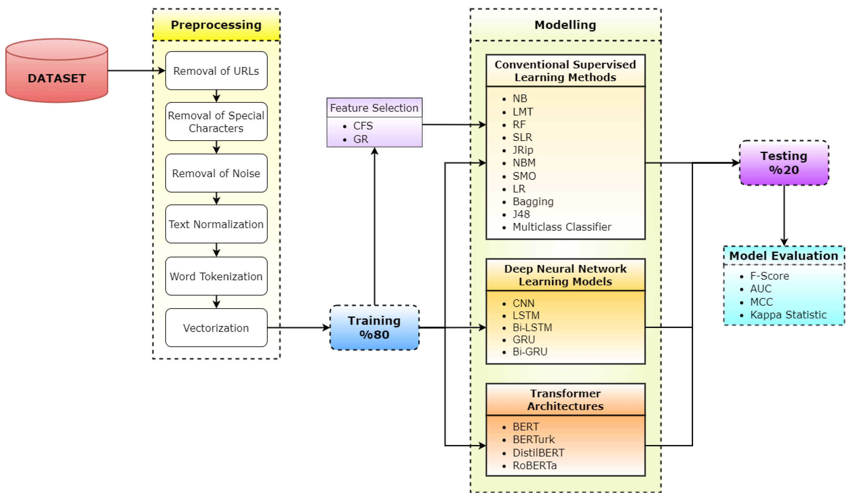
This section discusses the algorithms developed, the Turkish dataset established for use in the context of this study, and the techniques utilized to organize the dataset. This study entailed developing models using deep learning, machine learning, and transformer model-based algorithms and evaluating their performance outcomes. Figure 1 displays the pipeline of the workflow and its complete architecture, consisting of three stages.

In Algorithm 1, the fundamental stages of the workflow and its entire architecture have been briefly summarized as pseudo-code.

Algorithm 1: Pseudo-code of the proposed scheme.

//Input //Turkish Software Requirements Classification (TSRC) Dataset[]: array[TSRC_Dataset]; MLAlg[]: array[NB,LMT,RF,SLR,JRip,NBM,SMO,LR,Bagging,J48,MulticlassClassifier]; fsMLAlg[]: array[CFS,GR]; DLAlg[]: array[CNN,LSTM,Bi-LSTM,GRU,Bi-GRU]; TLAlg[]: array[BERT,BERTurk,DistilBERT,RoBERTa]; //Output MLResults_Fscore[]: array; fsMLResults_Fscore[]: array; DLResults_Fscore[]: array; TLResults_Fscore[]: array; //Preprocessing Dataset = (RemovalOfURLs(Dataset)); Dataset = (RemovalOfSpecialCharacters(Dataset)); Dataset = (RemovalOfNoise(Dataset)); Dataset = (TextNormalization(Dataset)); Dataset = (WordTokenization(Dataset)); Dataset = (Vectorization(Dataset)); //Training Split the TSRC_Dataset into 80% train and 20% test MLTrainResults[]: array [MLAlg[Dataset]]; fsMLTrainResults[]: array[fsMLAlg[Dataset]]; DLTrainResults: array[DLAlg[Dataset]]; TLTrainResults: array[TLAlg[Dataset]]; //Modeling and Testing int position = 0; while (position < Dataset[].length) {    for (i = 0; i < MLAlg.length; i++) {       MLResults_Fscore[] = Test(MLTrainResults[]);       fsMLResults_Fscore[] = Test(fsMLTrainResults[]); }    for (i = 0; i < DLAlg.length; i++) {       DLResults_Fscore[] = Test(DLTrainResults[]); } for (i = 0; i < TLAlg.length; i++) {       TLResults_Fscore[] = Test(TLTrainResults[]); } position++; } //Model Evaluation printf(“Machine Learning F-score Results”); for (i = 0; i < MLAlg.length; i++) {      printf(MLResults_Fscore[i]); } printf(“Machine Learning with Feature Selection F-score Results”); for (i = 0; i < fsMLAlg.length; i++) {      printf(fsMLResults_Fscore[i]); } printf(“Deep Learning F-Score Results”); for (i = 0; i < DLAlg.length; i++){      printf(DLResults_Fscore[i]); } printf(“Transfer Learning F-Score Results”); for (i = 0; i < TLAlg.length; i++){      printf(TLResults_Fscore[i]); }

The approach considered in the study consists of five consecutive steps. While the dataset was assessed in the first step, the second step focused on the preprocessing tasks performed on the dataset. In the third step, the algorithms were trained with 80% of data: (i) conventional machine learning algorithms with feature selection applied and (ii) deep learning algorithms and transfer learning algorithms. The results of the experiments were evaluated in the fourth step with performance metrics. In the last step, the performance results obtained after running the tests were analyzed.

3.1. Subsection Dataset Collection and Preprocessing

Apart from the algorithm used and the model developed in artificial intelligence approaches such as machine learning and deep learning, the dataset is also a significant aspect in determining the performance outcome. In addition, the samples in the dataset should accurately reflect the subject and be adaptive and functional in real life. Considering this information, this study identified the requirements by analyzing the real software projects developed for various platforms and sectors. Two subject-matter experts then labeled these requirements as FR and NFR. During the labeling process, this study utilized the majority voting technique and retained the labels for which both experts reached the same conclusion while reviewing those for which they made opposite decisions. Figure 2 shows the distribution of the dataset labeled FR and NFR.

There are a total of 4600 requirements in the dataset, which include requirements for real-world software projects based on Windows, web, and mobile platforms. To the best of our knowledge, there is no study on the automatic classification of software requirements in the Turkish language; we created the dataset in Turkish.

Table 2. Requirements examples from the dataset.

Sample Sentences	English Translation of Sentences	Label
Sistem olayları mevcut zamandan farklılıklarına göre renklendirecektir.	The system will color events according to their difference from the current time.	FR
Kullanıcı Canlı Döviz Takip Uygulaması üzerinden bir bankanın döviz bilgilerini anlık takip edebilecektir.	The user will be able to instantly follow the currency information of a bank through the Live Currency Tracking application.	FR
Sosyal doku analizi uygulaması üzerinde eklenen kullanıcı bilgileri saklanacaktır.	User information added on the social texture analysis application will be stored.	FR
RemMed uygulaması üzerinden kullanıcı sağlık günlüğünü doktoru ile paylaşabilecektir.	The user will be able to share his health diary with his doctor through the RemMed application.	FR
Kullanıcı e-posta ve şifresi ile sisteme giriş yapabilecektir.	The user will be able to login to the system with his e-mail and password.	FR
Seyahatname uygulaması tarafından kullanıcının yaptığı hatalara karşın doğru hata mesajları verilmelidir.	Correct error messages should be given by the Travelogue application for the mistakes made by the user.	NFR
Mobil tabanlı pazaryeri uygulaması aynı anda en az 1000 kullanıcıya hizmet verebilecektir.	The mobile-based marketplace application will be able to serve at least 1000 users at the same time.	NFR
Network alt yapısı sistem kaynaklarının her biri için ortalama en fazla %50′sini kullanmalıdır.	The network infrastructure should use at most 50% of the system resources on average.	NFR
Hesabını Bil uygulaması üzerinde yer alan ekranların yenilenme süresi en fazla 5 saniye olacaktır.	The refresh time of the screens on the Know Your Account application will be a maximum of 5 s.	NFR
Geliştirilecek oyun programı üzerindeki ekran kontrolleri oyuncunun oyunu oynamasına engel olmayacak büyüklükte olmalıdır.	The screen controls on the game program to be developed should be large enough to not prevent the player from playing the game.	NFR

shows examples of the requirements in the dataset.

As the created dataset is in a natural language format, a data preprocessing step was applied in the study to convert the data into a format that algorithms could process. The initial stage in natural language processing studies is to execute the data preprocessing after creating the dataset. In this stage, natural language is converted into a machine-understandable text format to prepare algorithms for use in artificial intelligence techniques. Data preprocessing is as crucial as creating the dataset since the data quality is directly related to the predictive performance of the generated algorithm to be real-like. With this objective in mind, the current study applied noise removal and text normalization—including removal of punctuation, special characters, stopwords, and case conversion—preprocessing techniques such as tokenization and vectorization after the dataset creation process [13]. Data preprocessing is necessary for automatic natural language processing when addressing morphologically complex languages like Turkish. In this context, ML algorithms need additional feature engineering applications after the aforementioned preprocessing steps. As a result, this study additionally applied a feature selection method to the dataset to achieve this outcome.

3.2. Feature Selection

Artificial intelligence techniques such as data mining and natural language processing have been developed to control the data spread and extract accurate information from the data. In this context, the feature selection aims to create simpler and more comprehensible models to improve data mining performance and prepare clean and intelligible data [14].

A feature potentially refers to an option in each column in the dataset that characterizes the data. It is possible to classify text by the options defining that text. Considering the features that best describe the data for a successful classification process is ideal. Hence, it is essential to consider the features that best characterize the data to acquire real-like results in text classification tasks. Feature selection refers to handling the options that reflect the data more by ignoring the same features in the entire dataset or those that do not retain a distinctive effect on the overall dataset. The feature selection strategies aim to increase the prediction performance and hasten the learning process by reducing the dimensionality [15].

High-quality features contributing to computation from the data feature space and improving performance are employed to create a feature subset in machine learning algorithms using feature selection techniques, which are often employed in data preprocessing [16]. The study also utilized correlation-based feature selection (CFS) and gain ratio (GR) feature selection techniques.

CFS is a multivariate filter approach selecting subsets of unrelated but highly correlated features with the class [17]. A heuristic evaluation function is used for the ranking process of the feature subsets in correlation-based feature selection. While more significant features are defined as highly correlated in the training and testing process of the prediction model, the procedure ignores low-correlation features. Furthermore, the prediction model eliminates the unnecessary options [18].

Information gain is calculated for all features in the GR technique [19]. Hence, the features performing at least as much as the average information gain and achieving the best gain ratio are selected. GR outperforms the information gain measure in terms of both accuracy and classifier complexity [20].

3.3. Conventional Machine Learning Methods

Machine learning is a broad discipline that spans information technology, statistics, probability, artificial intelligence, psychology, neurobiology, and many other disciplines. It also refers to teaching computers to think like humans while generating the field of statistics and fundamental statistical-computational theories of learning processes. Machine learning algorithms are categorized into groups, including supervised learning, unsupervised learning, semi-supervised learning, and reinforcement learning, depending on the way of seeking a solution to a problem [21,22]. This study used the supervised learning method. Classes are manually separated and labeled beforehand in supervised learning algorithms. Mathematical models created with machine learning algorithms are trained and tested, aiming to achieve the highest prediction performance. This study utilized the Weka library to test conventional algorithms. It also used many algorithms in this library during the experimental design and selected the best-performing algorithms. Figure 1 presents a list of ML algorithms, and the following section briefly describes these algorithms.

The Naïve Bayes (NB) classifier is a powerful machine learning algorithm based on Bayes’ theorem. It assumes independence from any condition or event, making it easy to implement and suitable for large datasets [23]. This method calculates the probability of a sample belonging to a class independently of others, identifying the highest probability class for classification. NB is widely used in text mining.

Naïve Bayes Multinomial (NBM) is an advanced version of the current Naïve Bayes classifier that calculates the frequency of each word. It is well-established that frequency is highly effective in classifying the text into different categories. Therefore, the NBM algorithm is considered one of the best in text classification [24].

The Logistic Regression Tree (LRT) is a decision tree structure that integrates Logistic Regression principles. Each node in the tree uses a unique logistic algorithm, resembling conventional decision trees with child nodes. Predictions are made by performing logistic calculations at these nodes, comparing feature values to threshold values [25].

Sequential Minimal Optimization (SMO) is a popular classification algorithm used for training support vector machines in supervised machine learning. It resolves quadratic programming problems in SVM through an iterative algorithm that breaks the optimization task into smaller subproblems, which are solved analytically to avoid numerical QP optimization [26].

Random Forest (RF) is a machine learning algorithm that enhances prediction accuracy by utilizing multiple decision trees on different subsets of a dataset and averaging their results. Instead of relying on a single tree, it aggregates predictions from multiple trees. At each tree node, conditions are compared with one or more input data features. Each tree provides a class prediction, and the algorithm selects the most frequently predicted class as the final prediction. RF performs exceptionally well on unbalanced datasets, with very few classification errors [27].

Logistic Regression (LR) is a versatile technique used for classifying both linear and nonlinear data. It is particularly employed in models with binary responses, often represented as 0/1. In this representation, ‘1’ signifies success, and ‘0’ denotes failure. The values of 1 and 0 can vary based on the study’s objectives. In binary classification, one class is labeled as ‘1’, and the other is labeled as ‘0’. Logistic Regression is a machine learning algorithm that involves multiplying the input by weight values to make predictions [28].

Simple Logistic Regression (SLR) performs outstandingly with linear data, whereas it may perform poorly with nonlinear or complex data. It also fails to address datasets with missing data [27].

Bagging is an algorithm that operates using the ensemble learning method. Each ensemble model is trained on a subset of the current dataset. Because the models work independently, it is possible to train them concurrently. Combining the decisions of the classifiers results in the classification of a new test instance by the ensemble model. The goal is to achieve better performance by using multiple classifiers [29].

JRip is one of the most used machine learning algorithms. Its operation principle involves analyzing classes as they expand and creating the initial set of rules for these classes with gradually decreasing error rates. It is ideal to use this algorithm to classify all samples in each dataset in the training data and to search for a set of rules that apply to all members of that dataset. It then proceeds to the next class and repeats the procedure until all classes have been evaluated [30].

J48 is a machine learning classifier that handles features with missing values, performs rule derivation, and manages continuous-valued feature ranges. This algorithm generates rules to establish a distinct data identity. The purpose of using this classifier is to iteratively expand the decision tree until it achieves a balance between versatility and accuracy [30].

A Multiclass Classifier is a supervised classification algorithm used when there are more than two possible outcomes in a classification task [31]. It operates based on ensemble theory. Initially, several algorithms are trained on a subset of data, and then the algorithms with the highest performance are evaluated. This classifier is considered successful in machine learning because its testing procedure involves multiple algorithms, each of which is assessed for effectiveness.

3.4. Deep Neural Network Learning Models

Deep learning is a significant and trending topic in the artificial intelligence discipline. The development of deep learning techniques resides in exemplifying the human brain, nervous system, and its functions [32,33]. Deep learning is an extraction process of knowledge from data utilizing Artificial Neural Networks inspired by nerve cells and multi-layered hidden architectures. Data is transferred through several layers in a deep learning algorithm, with each layer progressively extracting features and sending data to the next layer. The initial layers extract low-level features and combine them with subsequent layers to create a comprehensive representation.

The conventional machine learning classification task entails preprocessing, feature extraction and selection, and classification/model setting stages. The correct feature selection is a primary factor in the high prediction performance of machine learning systems. As illustrated in Figure 3, on the other hand, deep learning models concurrently perform feature extraction, feature selection, learning, and classification procedures. Such versatility of the deep learning algorithms makes it advantageous for executing numerous tasks.

Deep learning techniques using deep neural networks have gained popularity in parallel with the advancements in high-performance computer opportunities. Several newly developed techniques and numerous studies applying these methods to address various challenges have been increasing gradually. These techniques are still in use today and are broadly applicable to diverse branches of natural language processing. Due to the neural networks’ capacity to learn representations with various degrees of abstraction, deep learning has been applied to natural language processing to attain cutting-edge performance in numerous tasks, including language building [34]. Convolutional Neural Networks, Long Short-Term Memory, Bidirectional Long Short-Term Memory, Gateway Repetitive Units, and Bidirectional Gateway Repetitive Units are all deep learning algorithms.

3.4.1. Convolutional Neural Networks

Convolutional Neural Networks (CNNs), a variety of traditional feed-forward neural networks, are extensively used in image recognition and have more recently drawn interest in natural language processing. In natural language processing, CNNs use a sentence representation that keeps the word order completely preserved. As a result, CNNs may eventually learn and recognize patterns consisting of strings of words that span more than one word in a sentence. This context makes CNN compatible with pattern recognition-related tasks. As depicted in Figure 4, a simple CNN network consists of embedding, convolution, pooling, dropout, fully connected, and output layers [35,36].

The input/word embedding layer is the component responsible for creating a vector representation of the input sentence and converting it into a 2D matrix [36]. However, the convolution layer is where two-dimensional filtering procedures are performed on the input matrix to extract the feature map. The filtering procedure is applied to each field in the input matrix, which is referred to as convolution. Each convolution serves as a neuron, computing the scalar product of its weights and the regional input, and, subsequently, the activation function [37] converts into a single feature. The features of each convolution are collected in a feature map for each filter [27]. The pooling layer follows the convolution layer and performs down-sampling and dimensionality reduction on the input data, reducing the number of connections in the network. Its primary purpose is to alleviate the computational load and address overlearning problems. The pooling layer also defragments various image dimensions and enables CNNs to recognize objects even if their shapes are distorted or viewed from different angles [34]. The dropout layer is one of the typical systems functioning in neural networks to ensure the rarefication and generalization of the model. This layer also lessens the number of training iterations needed, hastens training procedures, and provides trained networks with lower error rates [8]. The fully connected layer, also referred to as the dense layer, is used for the final prediction. This layer passes the data through a series of entirely interconnected neurons. As a result, it predicts under which class the data falls [35].

3.4.2. Long Short-Term Memory

Long Short-Term Memory (LSTM) is an advanced version of recurrent neural networks. LSTM models are more effective at retaining and utilizing information in longer sequences [34]. In an LSTM architecture consisting of neural network layers, the input data from the processing layer and the output data from the preceding layer are stored in memory in an LSTM architecture, consisting of neural network layers. Thus, it enables us to make predictions based on current and previous data. The LSTM also checks the timing of impending data access to memory and its exit. In principle, input, forget, and output are the three building blocks of the LSTM architecture, and the information flow manifests through these blocks. It can also learn about long-term dependencies.

3.4.3. Bidirectional Long Short-Term Memory

Bidirectional Long Short-Term Memory (Bi-LSTM) is an extension of the LSTM architecture that addresses the drawbacks of standard LSTM models by considering both past and future context in sequential modeling tasks. While conventional LSTM models only process input data in the forward direction, the Bi-LSTM model overcomes this limitation by training the model in both directions. A standard Bi-LSTM architecture has two parallel layers that process the input string forward and backward. This bidirectional processing enables the model to capture information from past and future contexts, providing a more comprehensive understanding of temporal dependencies within the sequence [34].

3.4.4. Gated Recurrent Unit

The Gated Recurrent Unit (GRU) is a type of Recurrent Neural Network (RNN) inspired by the functionality of LSTM. The GRU has two ports—the reset and update ports—and displays the entire status every time without a control mechanism. Resetting allows for erasing unnecessary information. The update port, on the other hand, controls the quantity of the data transferred from the previous remote state. Actual activation is calculated as a linear interpolation of previous and candidate activations [38].

3.4.5. Bidirectional Gated Recurrent Unit

A Bidirectional Gated Recurrent Unit (Bi-GRU) consists of two GRUs. These GRUs have opposite directions and independent parameters. The advantage of Bi-GRU is that it can analyze the relationship between contextual sentences. In this manner, it can make the right decisions about the meaning of each sentence, potentially extracting the text features most closely related to the original one [39].

3.5. Transformer Architectures

Transformer-based language models, which reside on the most advanced language models, are a unique class of artificial intelligence that analyzes natural language texts to mimic human language processing. Transformer-based models provide a more thorough interpretation of related words by considering the context of the processed words. These are pre-trained language models, in other words, they are a tested solution for a wide range of natural language processing tasks. In this context, a language model based on transformers is initially trained on many texts before being finely tuned on task-specific data [40,41]. BERT, BERTurk, DistilBERT, and RoBERTa are transformer-based models.

3.5.1. BERT

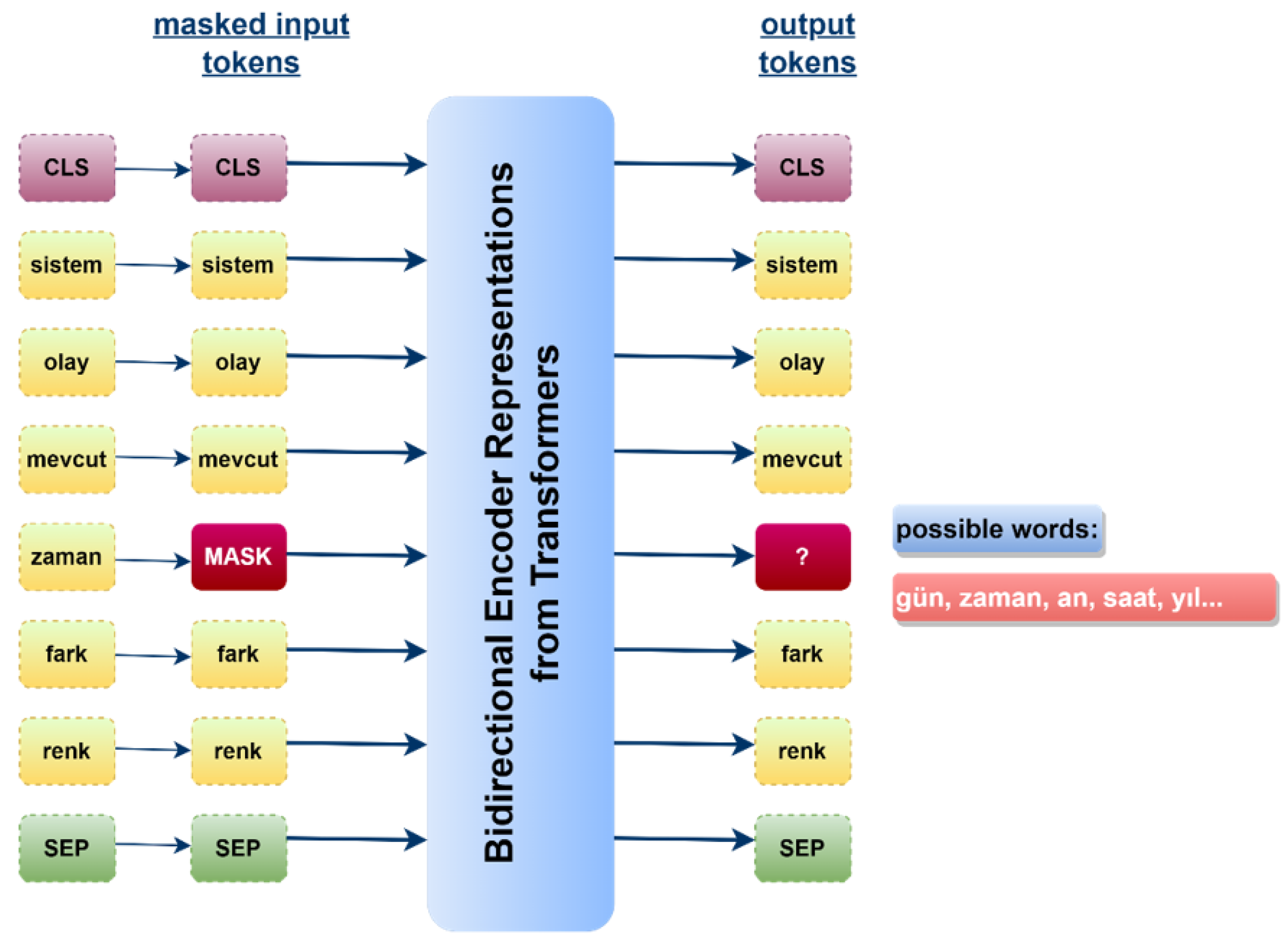
The acronym BERT—Bidirectional Encoder Representations from Transformers—is a transformer-based language model developed by Google with the architecture illustrated in Figure 5. It consists of two stages: encoder and decoder. The encoder produces an output after sequentially processing the input in coding layers. The decoding layers subsequently process this output. BERT was trained on 16 GB of texts from BooksCorpus datasets and English Wikipedia. When BERT analyzes words in a text, it considers its morphology and context. BERT potentially scrutinizes language with “Masked Language Modeling” and “Next Sentence Prediction” mechanisms. In masked language modeling, the algorithm initially ignores (masks) a word anywhere in the input sentence; accordingly, it attempts to predict this masked word within the sentence by analyzing the pre- and post-texts of the ignored/masked word. The mechanism used to predict the next sentence follows a similar approach. Instead of any word in the sentence, the model randomly masks a sentence in the input text and subsequently analyzes the pre- and post-sentences to predict the masked sentence. Thus, this model outperforms many other language models with this feature [42]. Since the BERT is a previously trained model with big datasets, this process makes it substantially faster. Because only preliminary training and fine adjustment are sufficient since the development of the model will reside on a pre-existing model.

3.5.2. BERTurk

When initially using the BERT model in natural language processing, there were diversely developed variants of the BERT architecture for numerous issues or different languages. The BERTurk model trained with Turkish data to analyze Turkish texts is also one of these variants. Since they share the same architecture as BERT, the BERTurk-originated models are also more performant and faster than other natural language processing models. Furthermore, using a ready-made model would significantly impact the performance via correctly operating the pre-processing and fine-tuning by the model requirements [43].

3.5.3. DistilBERT

DistilBERT is also a variant of the BERT architecture, much like BERTurk. While the purpose of developing BERTurk was for a different language than BERT, DistilBERT involved a model modification. It primarily uses the BERT’s initial version architecture as a base, replacing heavier architectures with more parameters with a light version of the same architecture with fewer parameters. Hence, it reduces the number of layers by half in the BERT-based model, eliminating identifier embeddings and poolers to yield a significantly faster and smaller version of BERT for widespread use [44]. The model also applies dynamic masking and ignores next-sentence predictions. DistilBERT aims to generate a faster-running version of BERT [42].

3.5.4. RoBERTa

With an almost similar architecture to BERT and built on the same language masking strategy, RoBERTa (Robustly Optimized BERT Pretraining Approach) is an optimized method for pre-training a self-supervised NLP system [45]. The main difference between them is that BERT uses static masking while RoBERTa uses dynamic masking [44]. RoBERTa allows for better performance by changing the basic hyperparameters in the BERT model.

3.6. Evaluation and Statistical Validation Metrics

This study employed frequently used performance evaluation metrics—F-score and AUC—and statistical validation metrics—MCC and Kappa—to evaluate the performance results of models developed with artificial intelligence approaches.

3.6.1. Performance Metrics

A set of metrics is required to compare and evaluate the results of algorithms developed for a classification problem. Confusion matrix (CM) is the primary instrument to acquire the essential metrics for the binary classification of software requirements as functional and non-functional. True-positive (TP) and true-negative (TN) depicted in Figure 6 are regarded as correct predictions, whereas false-negative (FN) and false-positive (FP) are considered incorrect predictions [43].

Finding the precision and recall values is necessary to calculate the F-score metric. The precision value defines the number of FR-predicted requirements for the actual FR class presented in Figure 6, and it is calculated with the formula in Equation (1). In contrast, the recall value expresses the number of FR-predicted requirements of all FR requirements in the dataset, and it is calculated with the formula in Equation (2). Using precision and ecall values, the F-score [46] is calculated by the formula in Equation (3).

$$\mathrm{P}\mathrm{r}\mathrm{e}\mathrm{s}\mathrm{i}\mathrm{c}\mathrm{i}\mathrm{o}\mathrm{n}=\frac{\mathrm{T}\mathrm{P}}{\mathrm{T}\mathrm{P}+\mathrm{F}\mathrm{P}}$$

(1)

$$\mathrm{R}\mathrm{e}\mathrm{c}\mathrm{a}\mathrm{l}\mathrm{l}=\frac{\mathrm{T}\mathrm{P}}{\mathrm{T}\mathrm{P}+\mathrm{F}\mathrm{N}}$$

(2)

$$\mathrm{F}\text{-}\mathrm{s}\mathrm{c}\mathrm{o}\mathrm{r}\mathrm{e}=2\ast \frac{\mathrm{P}\mathrm{r}\mathrm{e}\mathrm{s}\mathrm{i}\mathrm{c}\mathrm{i}\mathrm{o}\mathrm{n}\ast \mathrm{R}\mathrm{e}\mathrm{c}\mathrm{a}\mathrm{l}\mathrm{l}}{\mathrm{P}\mathrm{r}\mathrm{e}\mathrm{s}\mathrm{i}\mathrm{c}\mathrm{i}\mathrm{o}\mathrm{n}+\mathrm{R}\mathrm{e}\mathrm{c}\mathrm{a}\mathrm{l}\mathrm{l}}$$

(3)

The maximum appropriate value for an F-score is 1.0, indicative of perfect precision and recall, while the minimum achievable value is 0, when either precision or recall equals zero. Therefore, for a classification problem, the algorithms are more successful as their F-scores approach ‘1’. Since the definition of the F-score is the harmonic average of precision and recall values, it averts outliers from affecting performance in unbalanced datasets. Additionally, the dataset in the current study was partly unbalanced; as a result, the study identified the F-score as the evaluation metric.

AUC, or ‘area under the ROC curve’, is the measure of the area under the ROC curve where the AUC takes values between 0 and 1. Generally, an AUC of 0.5 suggests no discrimination, while values between 0.7 to 0.8 are considered acceptable, and 0.8 to 0.9 is regarded as excellent for a classification problem.

3.6.2. Statistical Validation Metrics

Matthews Correlation Coefficient (MCC) and Kappa statistics-based metrics are ideal for evaluating algorithms developed for prediction problems. All values in the complexity matrix are used in the calculation to assess the performance of a model with the Matthews Correlation Coefficient metric [47]. Considering the correlation between the actual data and the predicted data, Equation (4) is employed to calculate this matrix. The minimum and maximum limits are ‘−1’ and ‘+1’, respectively, meaning that the performance increases and the predictions are correct as the value approaches ‘1.’

$$\mathrm{M}\mathrm{C}\mathrm{C}=\frac{(\mathrm{T}\mathrm{P}\ast \mathrm{T}\mathrm{N})-(\mathrm{F}\mathrm{P}\ast \mathrm{F}\mathrm{N})}{\sqrt{(\left(\mathrm{T}\mathrm{P}+\mathrm{F}\mathrm{P}\right)\ast \left(\mathrm{T}\mathrm{P}+\mathrm{F}\mathrm{N}\right)\ast \left(\mathrm{T}\mathrm{N}+\mathrm{F}\mathrm{P}\right)\ast (\mathrm{T}\mathrm{N}+\mathrm{F}\mathrm{N}\left)\right)}}$$

(4)

Kappa statistic indicates the correspondence between the actual and predicted values. It also considers whether this correspondence is by chance. As in the MCC metric, the minimum and maximum values vary between ‘−1’ and ‘+1’, respectively. As a result, the model is more successful as the Kappa value approaches “1” [48], whereas “0” indicates that the existing correspondence is by chance.

4. Experiments and Discussion

This section explores the answers to the following research questions (RQ1, RQ2, RQ3, and RQ4):

• RQ1: How successful are conventional supervised learning methods in identifying software requirements as functional and non-functional?
• RQ2: How successful are deep learning methods in identifying software requirements as functional and non-functional?
• RQ3: How successful are transfer learning models in identifying software requirements as functional and non-functional?
• RQ4: Which of the conventional supervised learning, deep learning, and transfer learning methods is more successful in classifying software requirements?

4.1. Procedure Followed in Experiments

In principle, experimental studies involve three stages: machine learning algorithms, deep learning algorithms, and classification of transfer learning methods and software requirements as FR and NFR. All of the experiments utilized in the dataset are provided in Section 3. While performing experimental studies, the dataset was divided into two parts, 80% and 20% for training and testing, respectively.

4.2. Experimental Results

The study initially used the Weka tool for classification experiments with machine learning algorithms. It also experimented with all machine learning algorithms available on Weka and revealed the findings of the 11 most successful algorithms provided in

Table 3. F-score and AUC value of conventional algorithms.

Algorithm	F-Score	AUC
NB	0.830	0.899
LMT	0.914	0.959
RF	0.909	0.961
SLR	0.899	0.956
JRip	0.901	0.887
NBM	0.928	0.970
SMO	0.913	0.902
LR	0.888	0.933
Bagging	0.863	0.930
J48	0.826	0.879
Multiclass Classifier	0.888	0.933

.

The data analysis presented in Table 3 revealed that the models developed with machine learning algorithms yielded comparable performance results. Of all the models, the model developed with the Naïve Bayes Multinomial was the highest-performing model, with a 92% F-score and 97% AUC value. The model developed by the LMT algorithm followed the Naïve Bayes Multinomial algorithm with a 91% F-score and 95% AUC value. In addition, the models created by the Logistic Regression and Multiclass Classifier displayed the same performance level. Considering the algorithm with the lowest performance among the 11 algorithms analyzed, however, it was the model developed by J48, with an 82% F-score and 87% AUC value.

In addition to conventional machine learning algorithms, feature selection techniques have been applied to the same algorithms to improve performance. In this context, the study used CFS and GR feature selection methods to identify their effects on performance results and displayed the outcomes in

Table 4. F-score and AUC value of conventional algorithms with feature selection methods.

Algorithm	F-Score		AUC
	CFS	GR	CFS	GR
NB	0.787	0.856	0.895	0.897
LMT	0.842	0.816	0.91	0.962
RF	0.842	0.805	0.909	0.962
SLR	0.841	0.904	0.915	0.957
JRip	0.836	0.905	0.501	0.501
NBM	0.837	0.830	0.503	0.503
SMO	0.834	0.915	0.792	0.903
LR	0.845	0.891	0.917	0.929
Bagging	0.832	0.862	0.896	0.929
J48	0.751	0.821	0.786	0.883
Multiclass Classifier	0.845	0.830	0.917	0.929

.

The performance results of the feature selection algorithms in Table 4 indicated that they failed to generate any positive effect on the performance increase. However, the F-score relatively increased when the GR feature selection technique was applied to the model developed with SMO, Simple Logistic Regression, and the Naïve Bayes algorithm. Additionally, in two feature selection techniques, the performance of the model created by the Naïve Bayes Multinomial, which had the best performance in the prior trial, declined.

In the second stage, the study conducted experiments with CNN, LSTM, Bi-LSTM, GRU, and Bi-GRU deep learning algorithms and accordingly displayed the findings in

Table 5. F-score and AUC value of deep learning algorithms.

Algorithm	F-Score	AUC
CNN	0.937	0.918
LSTM	0.914	0.893
Bi-LSTM	0.907	0.881
GRU	0.926	0.911
Bi-GRU	0.915	0.901

.

The assessment of the models developed with deep learning algorithms revealed that the CNN algorithm was explicitly successful and outperformed other deep learning algorithms in classifying software requirements as FR and NFR.

This study also performed experiments to classify software requirements as FR and NFR using BERT, BERTurk, DistilBERT, and RoBERTa transfer learning methods and presents the results in

Table 6. F-score and AUC value of transfer learning methods.

Algorithm	F-Score	AUC
BERT	0.921	0.971
BERTurk	0.954	0.983
DistilBERT	0.918	0.968
RoBERTa	0.862	0.952

.

Finally, in the third stage, the analysis of the experimental study results related to transfer learning methods indicated that the model developed with the BERTurk algorithm delivered the highest performance with a 95% F-score.

The above experimental results show that conventional ML algorithms, even when combined with advanced pre-processing techniques such as feature selection, do not demonstrate appropriate results from an automatic FR-NFR identification point of view. As it is stated above, the limitation of conventional ML algorithms may be remedied through deep learners combined with word embeddings to some extent. Though deep learners on top of word embeddings show a relatively increased performance compared to conventional ML algorithms, they are limited in grasping contextual representations compared to newly developed transformer language models. This is particularly expressed in the literature, and it is also shown in the empirical results given in Table 3, Table 4, Table 5 and Table 6. In clearer terms, the F-score performances of nearly all transformers surpass the best performances of all algorithms. Though the transformer models except BerTURK are multilingual, they still show significant performances for the Turkish software requirement domain.

From a confusion matrix point of view, the best performances of three algorithms from each group are presented in Figure 7.

As observed in Figure 7, BerTURK is able to identify much more TP and TN values compared to CNN and NBM. Also, BerTURK shows better performance decreasing FP and FN values.

4.3. Statistical Validation Results

The previous section discussed the F-score and AUC metrics results of experimental studies conducted with machine learning, deep learning, and transfer learning approaches. In addition, it statistically evaluated the experimental results and used validation metrics MCC and Kappa to analyze them comprehensively. Accordingly, MCC and Kappa values were calculated for all experiments performed in all three stages.

Table 7. Statistical validation results of machine learning algorithms.

Algorithm	MCC	Kappa
NB	0.663	0.627
LMT	0.809	0.808
RF	0.797	0.794
SLR	0.775	0.772
JRip	0.779	0.778
NBM	0.841	0.843
SMO	0.806	0.806
LR	0.753	0.752
Bagging	0.694	0.691
J48	0.616	0.615
Multiclass Classifier	0.753	0.752

lists the MCC and Kappa values of the experiments conducted with machine learning algorithms, while

Table 8. Statistical validation results of machine learning algorithms with feature selection methods.

Algorithm	MCC		Kappa
	CFS	GR	CFS	GR
NB	0.787	0.856	0.507	0.626
LMT	0.842	0.816	0.640	0.816
RF	0.844	0.805	0.634	0.805
SLR	0.841	0.904	0.637	0.783
JRip	0.836	0.905	0.627	0.618
NBM	0.837	0.830	0.629	0.626
SMO	0.834	0.915	0.621	0.810
LR	0.845	0.891	0.646	0.759
Bagging	0.832	0.862	0.691	0.688
J48	0.751	0.821	0.431	0.601
Multiclass Classifier	0.845	0.834	0.646	0.759

displays the MCC and Kappa values calculated by applying future selection techniques to the same algorithms.

Table 9. Statistical validation results of deep learning algorithms.

Algorithm	MCC	Kappa
CNN	0.837	0.835
LSTM	0.801	0.802
Bi-LSTM	0.814	0.817
GRU	0.828	0.824
Bi-GRU	0.787	0.793

presents the MCC and Kappa values of experimental studies with deep learning algorithms.

Table 10. Statistical validation results of transfer learning methods.

Algorithm	MCC	Kappa
BERT	0.874	0.873
BERTurk	0.898	0.897
DistilBERT	0.857	0.854
RoBERTa	0.789	0.788

displays the MCC and Kappa values of experimental studies conducted by transfer learning techniques.

An overall assessment of Table 7, Table 8, Table 9 and Table 10 revealed that MCC and Kappa values supported the F-score and AUC values. As both metrics approach ‘1,’ the accuracy of the predictions is supported. Considering the three groups of experiments, the average MCC and Kappa values of 0.85, particularly in Table 10, statistically confirmed the accuracy of the results. As a result, it is viable to conclude that the algorithms provided consistent results.

This work shows promising results from the newly generated Turkish requirements dataset and the use of the point of view of the transformers. However, there are some limitations of the dataset, which can be shown in three aspects: (i) While creating the dataset, software requirements were obtained through Windows desktop, web, and mobile software projects. Therefore, the dataset can be generalized with the collection of software requirements from different software projects such as cloud computing, data science, blockchain, information security, embedded systems, wearables software development, DevOps, and video game development. (ii) The dataset can also be expanded with the addition of more samples increasing sample size above 4600. (iii) The dataset includes 3000 functional requirements and 1600 non-functional requirements. In this respect, it is a relatively unbalanced dataset. The dataset can be further extended with the addition of more non-functional requirements.

5. Conclusions

Just as the correct identification of business needs is crucial for successful software projects, defining and addressing these requirements is equally essential to satisfy the business needs explicitly, consistently, concisely, and summarily in the analysis documents in a way that is explicit to all stakeholders to comprehend and leave no room for argument. Furthermore, a thorough analysis and classification of these requirements is necessary to develop high-quality and reliable software. Checking whether the identified requirements retain sufficient detail, pose internal consistency with each other, and meet the business needs are also among the critical issues to consider during the requirements analysis procedure. Subsequently, these identified requirements should be classified into functional and non-functional requirements. The manual identification process of functional and non-functional requirements is a highly challenging task since they are likely to be confused when written in natural language. The lack of functional requirements in a system under a development process would result in system failure. Similarly, ignoring non-functional requirements would equally lead to troubles, such as project failure, corruption of system integrity, or cost increase.

This study performed experiments for the automatic classification of software requirements using artificial intelligence algorithms on a unique dataset created in the Turkish language for the first time. Since the documentation of these requirements was written in natural language in text form, the study operated natural language processing methods in addition to artificial intelligence approaches. The study additionally carried out experimental studies within its scope, using conventional machine learning algorithms, deep learning algorithms, and transformer models. As a result, it achieved successful and generalizable results in classifying software requirements as functional and non-functional. The Naïve Bayes Multinomial was the best performing algorithm—with a 92% F-score—among the models created using machine learning methods. The CNN algorithm, however, performed the best—with a 93% F-score—among the deep learning algorithms developed using Artificial Neural Networks. In addition, the dataset underwent a training process with transfer learning methods, which has recently been frequently used in natural language processing and achieved very high-performance results. Considering the transfer learning methods, the BERTurk algorithm achieved a generalizable classification success with an F-score of 95%. As a result, Figure 8 illustrates the algorithms with the highest performance values and the performance evaluation metrics of these algorithms in the experimental studies carried out in three stages to classify the software requirements.

Considering the performance evaluation metrics and statistical validation metrics, this study identified the most successful performance with the BERTurk algorithm. The classification of software requirements is a critical issue. The number of Turkish studies on this subject is insufficient in the literature. Therefore, an original dataset created by the samples gathered specifically from Turkish texts, various platforms (windows, web, and mobile projects), diverse sectors, and actual project requirements will significantly contribute to subject-related studies.