Article

Developing a Static Kinematic Model for Continuum Robots Using Dual Quaternions for Efficient Attitude and Trajectory Planning

School of Biomedical Engineering, Hainan University, Haikou 570228, China
*
Author to whom correspondence should be addressed.
Appl. Sci. 2023, 13(20), 11289; https://doi.org/10.3390/app132011289
Submission received: 11 September 2023 / Revised: 11 October 2023 / Accepted: 11 October 2023 / Published: 14 October 2023
(This article belongs to the Special Issue Recent Advances in Robotics and Intelligent Robots Applications)

Abstract

:
Kinematic modeling is essential for planning and controlling continuum robot motion. The traditional Denavit Hartenberg (DH) model involves complex matrix multiplication operations, resulting in computationally intensive inverse solutions and trajectory planning. Solving position and orientation changes in continuum robots using the double quaternion rule can reduce computational complexity. However, existing dual quaternion methods are direct equational transformations of DH rules and do not give a complete modeling process. They usually require more interpretability when applying continuum robot kinematic modeling. This paper uses the dual quaternion method to establish a kinematic model of a continuum robot. It uses a two-section continuum robot model to compare the advantages of dual quaternion and traditional modeling methods. In addition, this paper proposes a five-polynomial interpolation algorithm based on the dual quaternion method for trajectory planning of continuum robots. This method accurately models spatial bending and torsional motions of singularity-free continuum robots.

1. Introduction

Researchers have become increasingly enthusiastic about continuum robots in recent years because of their excellent mechanical properties when operating in unique environments. The continuum robot is a flexible, continuous, multi-segmented robotic system inspired by the skeletal structure of biological organisms. In contrast with conventional rigid multi-joint robots, continuum robots employ a soft, deformable structure composed of numerous interconnected and continuous flexible segments. These segments can be actuated internally or externally using stimuli such as gas, liquid, or motors, facilitating smooth, seamless, and flexible motion and deformation. For example, continuum robots can perform surgical operations under minimally invasive and non-invasive conditions of the human body [1,2,3,4], target detection and fault diagnosis in narrow intervals [5,6,7], and grasp targets in high-pressure underwater environments, such as the deep sea [8]. They were developed from studying structures in nature that can be freely bent, twisted, and elongated, such as the arms of octopuses, the tongues of mammals and reptiles, and the trunks of elephants [9,10,11]. The diversity of potential applications of the continuum robot leads to various designs [12], which are reflected in the structure and the matching drive. From the physical form, the continuum robot is divided into the following formats: a single flexible pipe or rod with uniform stiffness [13], a series of flexible concentric tubes [14], a series of parallel truss platforms [15], flexible continuum pipes with multiple open slots [16,17], and a plurality of elastic material disks stacked. Drive models include pneumatic, traction line, electrochemical, and other drive modes. However, they all exhibit continuum curvature in a continuum robot, i.e., a continuum changes curvature along the main chain’s length. Furthermore, unlike conventional manipulators, which consist mainly of rigid elements resulting in only changing themselves at discrete points in their structure, continuum robots can theoretically change any position in their system [18,19], which leads to challenging kinematic and dynamic modeling of continuum robots and further leads to difficulties in real-time dynamic control.
Continuum robots have widespread use in quasi-static environments where dynamic models may not be applicable [20]. Researchers have employed various approaches to solving the kinematics of continuum robots, such as utilizing motion combinations of fake rigid manipulators to simulate their motion and applying the Denavit–Hartenberg (DH) model, which was initially developed for rigid manipulators’ accuracy in emulating continuum robot behavior; kinematic and shape correspondence between super-redundant manipulators and desired spatial profiles have been introduced [21,22]. Recently, the incorporation of continuum curvature into a modified DH modeling procedure using differential geometry has provided a comprehensive approach to modeling continuum robots [23]. Building upon this work, the researcher has proposed the variable reality of the central axis, associating the driving variable with the central axis curve to modify and enhance existing ideas [11]. The Jacobian matrix of the model and the corresponding kinematic control method have also been discussed. However, special numerical treatment is required when approaching these models’ straight (zero-curvature) cross-section configuration. The researcher expanded the driver variables, employing the Taylor series to address this issue and, thus, preventing model invalidity at zero curvature [24,25,26]. Nevertheless, modeling a multi-system or multi-joint manipulator arm using the above modeling approach becomes difficult, as the method of obtaining the end pose by multiplying the pose matrix places a significant workload on the system, and the relationship between each part of the system and the global coordinate system must be constantly considered. To address the challenge of dealing with sections with nearly straight deformation, the researcher has proposed using dual quaternions to solve this problem. Although the dual quaternion method offers increased efficiency in representing changes in the position and spatial elements of the robot, the existing approach is directly converted from the DH rule based on mathematical rules without considering the perspective of manipulator motion. This leads to limited interpretability of the dual quaternion method when applied to the kinematic modeling of manipulators in scientific journal articles.
Building upon previous research, this paper explores the dual quaternion method from the standpoint of kinematics in order to tackle continuum manipulator problems. The solution is established based on the definition, and the merits of the dual quaternion method are emphasized by comparing its computational efficiency with traditional DH model-based algorithms. The paper is structured as follows. Section 2 introduces the operational rules of dual quaternions and derives the principles for representing spatial rotation and displacement using dual quaternions. Section 3 illustrates the modeling of forward and inverse kinematics for single and multiple joints employing the dual quaternion method using the standard continuum manipulator model. Section 4 corroborates the results through simulation and experimental testing. Finally, conclusions are drawn in Section 5.

2. Materials and Methods

2.1. Dual Quaternion Rule

Quaternions are fourth-order hypercomplex numbers often used to describe changes in four-dimensional hyperplanes and vectors in graphics. Quaternions are generally represented in the form a + b i + c j + d k , where a , b , c , and d are real numbers, and i ,   j , and k are basic quaternions. Quaternions can be composed of a scalar part and a vector part. q is a quaternion represented as q = r , v , where r is a scalar defined in the real number field, and v is a three-dimensional vector. q * is the conjugate of q , represented by q * = r , v . q 1 and q 2 are two quaternions. The result and outer product of those are shown in Equations (1) and (2). The product of two quaternions is called the Grassmann product and is denoted by the symbol .
r 1 , v 1 + r 2 , v 2 = r 1 + r 2 , v 1 + v 2
r 1 , v 1 r 2 , v 2 = r 1 r 2 v 1 v 2 , r 1 v 2 + r 2 v 1 + v 1 × v 2
The dual numbers are a system of hypercomplex numbers, which are expressions of the form c + d ε , where c and d are real numbers, and ε is a symbol taken to satisfy. When c and d are replaced by quaternions using real numbers, the dual numbers are called dual quaternions. A dual quaternion can be represented in the form of q ^ , which can be written as q ^ = q r + ε q d . Among them, q r and q d are two quaternions, respectively, referred to as the imaginary and real parts of dual quaternions. q * ^ represents the dual quaternion conjugate, as shown in Equation (3).
q * ^ = q r * + ε q d *

2.2. Dual Quaternion Representation of Rigid Body Motion

Rigid body motions describing elements of solid geometry, such as points, lines, and surfaces in space, can be represented by dual quaternions. As shown in Equation (4), this means that the dual quaternion is used to represent a straight line A that changes into a straight line B after rotation and translation in space, where A ^ and B ^ are the Plücker forms of straight lines A and B, respectively. q ^ is the dual quaternions representing the angle of rotation θ around axis l . It can also be written in the form of Equation (5), where the derivation process is given in Appendix A.
B ^ = q * ^ A ^ q ^
q ^ = cos θ 2 , sin θ 2 l & + ε d 2 sin θ 2 , sin θ 2 m + d 2 cos θ 2 l

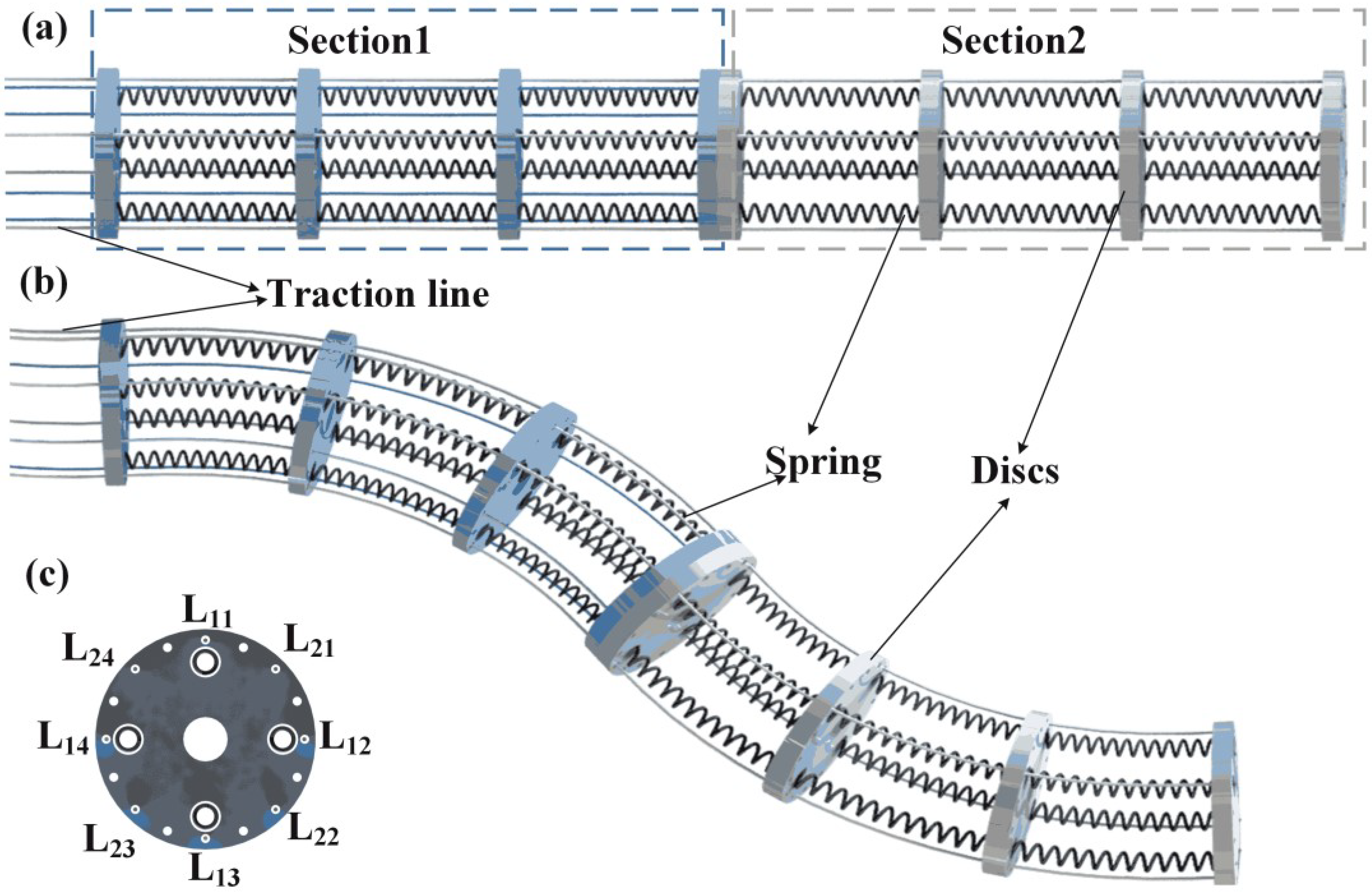
2.3. Physical Model of Continuum Robot

The general kinematic equations of a tendon-driven continuum robot arm are established. A specific example is presented to demonstrate the application of the derived kinematic equations, in which a tendon-driven continuum robot is considered. As illustrated in Figure 1, this continuum robot comprises two independent single-section manipulators, namely Section 1 and Section 2. Each manipulator section is constructed using a flexible disc as its primary structure, with the discs connected by springs, referred to as tendons. These tendons are secured at predetermined positions along the arc length of the robot. The end of the arm is equipped with a multi-traction line attached to the discs. By pulling these traction lines, a load is applied to the spring through the disc, resulting in the corresponding bending of the robot arm.

3. Kinematic Model of Continuum Robotics

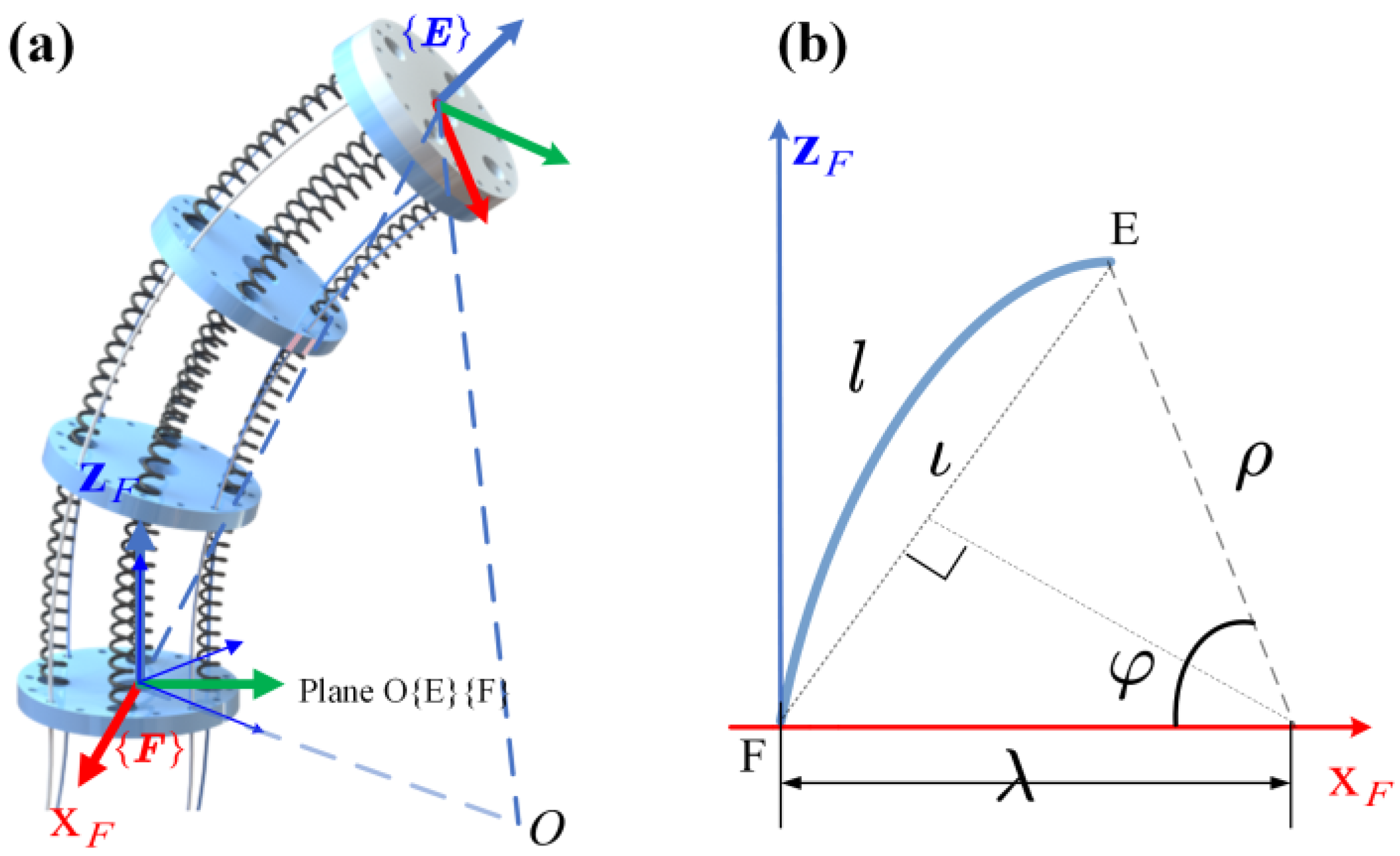
3.1. Center Axis Curve Parameters

Due to the arrangement of the tendons (discs and springs), the robotic arm is driven in line, and these continua exhibit a telescopic movement or bend into a circular shape. Therefore, the continuum arm’s central axis can be described in space precisely as a circular arc with a variable radius of curvature and length. As shown in Figure 2a, the diagram on the left shows the state of the continuum arm of the section when it is not driven, i.e., t = 0 . The central axis of the disc is a straight line with four drive lines of length L i j 0 j = 1 ,   2 ,   3 ,   4 . After the continuous manipulator is driven for time t, the state is shown in Figure 2b. The line length becomes L i j t j = 1 ,   2 ,   3 ,   4 . Let the change in rope length between the driven state and the undriven state be l i j   t , as shown in Equation (6).
l i j   t = L i j 0 L i j t
When the continuum arm is driven, the overall curve is assumed to be circular based on continuum curvature [24]. The radius of the curvature is described by ρ i 0 , , and the bending angle is described by φ i 0 , π 2 , which is on a plane that forms an angle δ i π , π with the x-axis as a whole in space. The curve parameters in joint space variables are given by Equations (7)–(9). A comprehensive derivation of these variables is provided in Appendix B.
φ i = 1 2 R i l i 4 l i 2 2 + l i 3 l i 1 2
δ i = arctan 2 l i 1 l i 2 l i 1 l i 3 1
ρ i = 2 l i 4 l i 2 2 + l i 3 l i 1 2 R i l i j

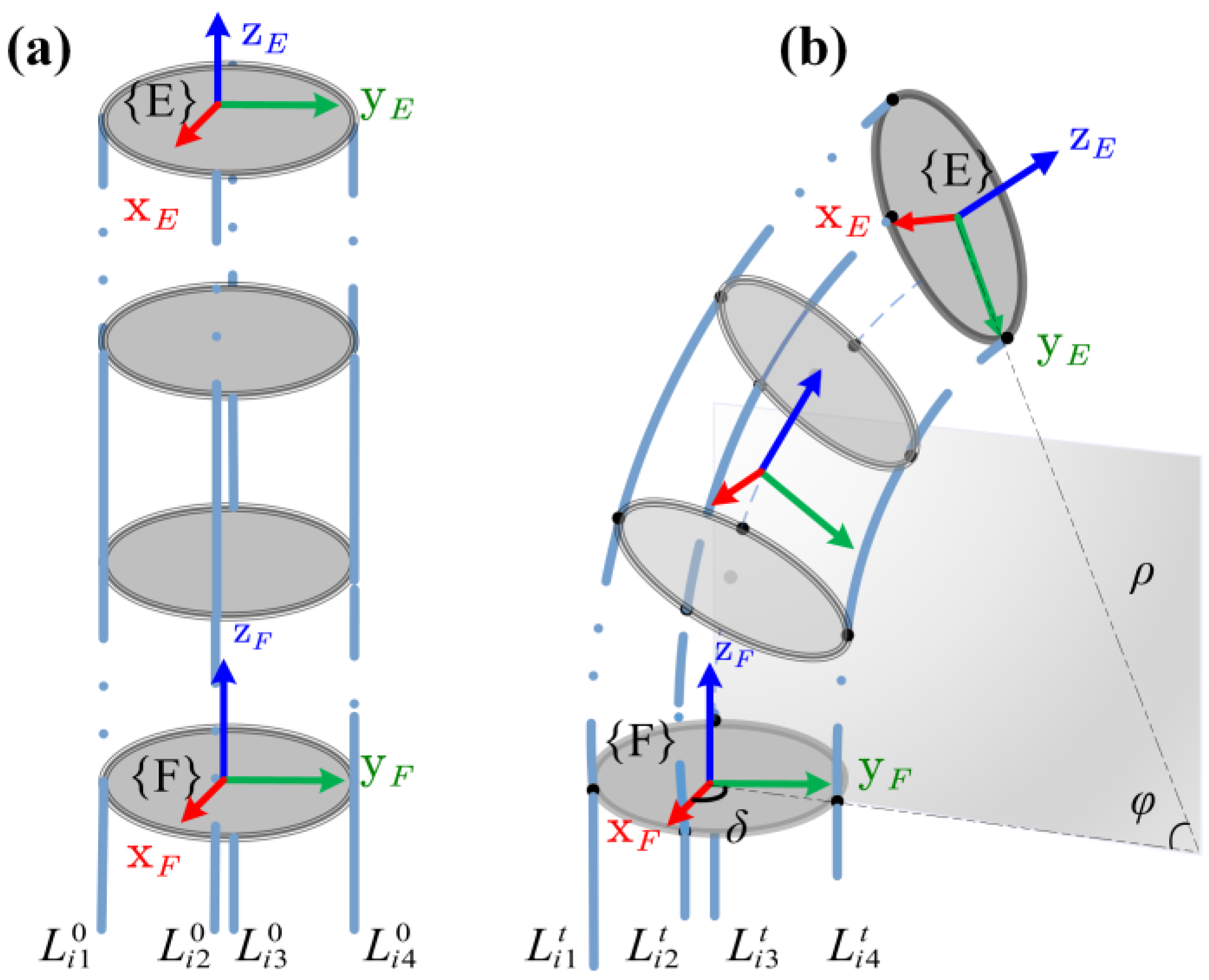
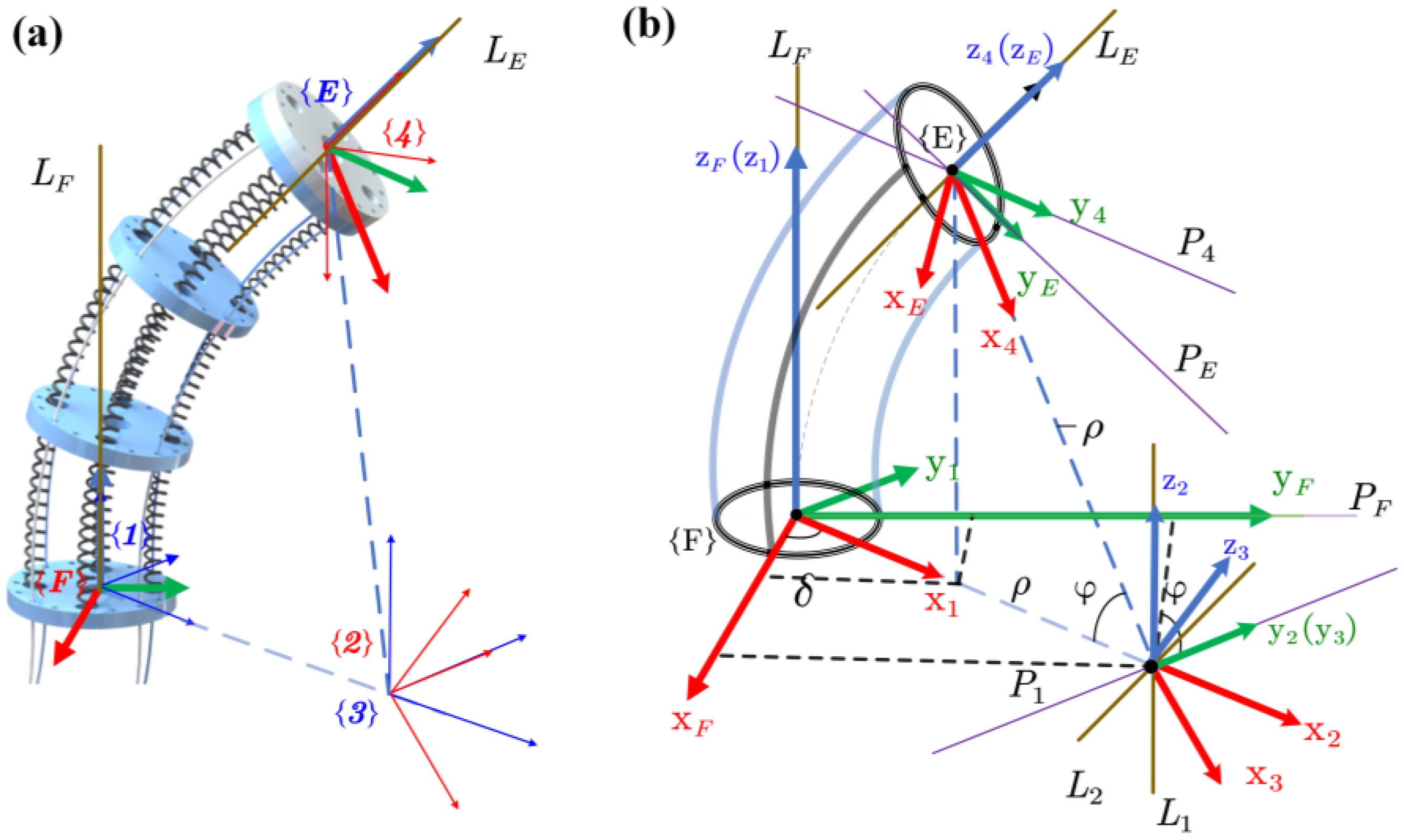
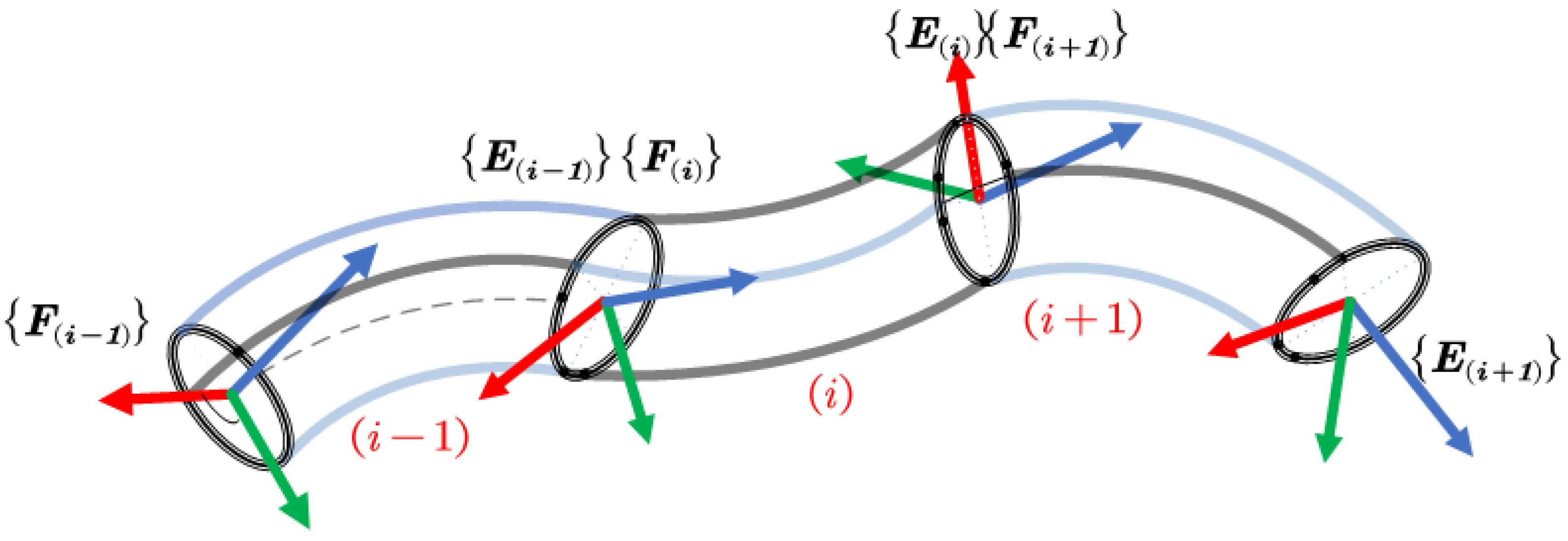
3.2. Coordinate Systems and Dual Quaternion Transformations of Points and Lines

A single-segment continuous robot is used to model using the dual quaternion method. The forward kinematics of the robot are to solve its end pose after driving. The physical model of the single-section robotic arm when driven is shown in Figure 3a.
As shown in Figure 3, if {F} and {E} are two reference frames, while q ^ E , q ^ F are the dual quaternion of those reference frames relative to a fixed coordinate system in space, then the relative position relationship between these two coordinate systems is called q ^ E F , which is represented by (10) and can be obtained from (4); a more detailed derivation process can be found in Appendix C.
q ^ E F = q ^ E q ^ F = c o s φ 2 , s i n δ s i n φ 2 , c o s δ s i n φ 2 , 0 & , 0 , 0 , 0 , ρ s i n φ 2
Let the lines in the front-end coordinate system {F} where the y -axis and z -axis lie be L F , P F and the direction vectors be l F and p F , respectively. By Euler’s theorem, the line L F in the coordinate system {F} becomes L 1 after a rotation around the z -axis and a translation ρ along the axis x 1 , and then L 2 around the axis y 2 , before a translation ρ along the new x 3 axis becomes L E in the coordinate system {E}. Similarly, P F can become P E . The moment vectors are m L , m P , respectively, which are expressed in the Plücker coordinate system as L F = l F , m L , P F = p F , m F . They can be expressed as L F ^ = l F + ε m L , P F ^ = p F + ε m F by a dual quaternion. Substituting (10) into (3), we can obtain the relationship between the straight line L F and L E on the coordinate system {F} and {E} as (11).
L ^ F = q ^ E F * L ^ E q ^ E F
Similarly, the relationship between P F and P E is (12).
P ^ F = q ^ E F * P ^ E q ^ E F
According to Plück’s law, the intersection points of the two are the position of the end coordinate system, and the pose can be expressed as l F   , p F   , l F × p F .

3.3. Kinematic Equations of Continuum Manipulator

As shown in Figure 4, three identical single-section robotic arms are connected in series to form an overall number:   i 1 ,   i ,   i + 1 . Then, the central axis is the z-axis direction on the front-end disk of this multi-section robotic arm. Next, establish a coordinate system and record it as {F}, and set up a coordinate system on the end disc with the central axis as the direction of the z-axis and record it as {E}. Assume that the center point at the top of the segment i + 1 is O , which is expressed as O E i + 1 = 0 , 0 in the coordinate system E i + 1 .
This point is denoted O F i + 1 = O F i + 1 , m F i + 1 in the coordinate system F i + 1 , because F i + 1 and E i are the same in space. Therefore, the end position of the robot arm in the section i + 1 can be expressed as O ^ E i in the end coordinate system of the section i .
O ^ E i + 1 = q ^ i + 1 i * O ^ E i q ^ i + 1 i
Similarly, the position of the central axis point of the front end of the multi-segment continuous arm in the coordinate system of the end of the first continuous arm is:
O ^ E i 1 = q ^ i + 1 i * q ^ i 1 i * O ^ E i + 1 q ^ i 1 i q ^ i + 1 i
Then the z and y axis directions of the frontmost position point are:
L ^ E i 1 = q ^ i + 1 i * q ^ i 1 i * L ^ E i + 1 q ^ i 1 i q ^ i + 1 i
P ^ E i 1 = q ^ i + 1 i * q ^ i 1 i * P ^ E i + 1 q ^ i 1 i q ^ i + 1 i
Through (15) and (16), the expression of the end position of the overall mechanical arm can be obtained in the first section of the robotic arm, and the complete forward kinematic equation can be obtained.

3.4. Control the Motion of the Robotic Arm through the End Position

In the previous section, the forward kinematic equations of the continuum arms were derived using the dual quaternion method. The Jacobian matrix of each part of the manipulator is first solved to solve the inverse kinematics numerically.
Let the expression of the Plücker form of the coordinates of a point P 0 in the coordinate system {0} be P ^ 0 , and the dual quaternion relationship between the coordinate system {0} and the coordinate system {1} is q ^ i .
Let the expression of the Plück form of the coordinates of a point P 0 in the coordinate system {0} be P ^ 0 , and the dual quaternion relationship between the coordinate system {0} and the coordinate system {1} is q ^ i , then the point can be expressed in the coordinate system {1} for (17).
P ^ 1 = Q 1 = q ^ i * P ^ 0 q ^ i
Writing (18) as a vector pattern gives (18).
Q 1 = Q 1 = 1 , ϑ 1 + 0 , ε x 1
The complete forward kinematics of i th section relative to {0}, denoted by Q i , is given by (19).
P ^ i = Q i = q ^ i * q ^ 1 * P ^ 0 q ^ 1 q ^ i
Write (19) as a vector, as shown in (20). Here ϑ ^ R 4 is the rotation and x ^ R 4 is the displacement.
Q i = Q 1 Q i = 1 , ϑ 1 , 2 i + 0 , ε x 1 , 2 i
Q i = Q 1 Q 2 Q i = Q i 1 Q i
Putting q ^ = q r , ε q d into (21), we can obtain (22) and (23), which are the dual quaternion representations of the position and pose matrix of the i th robotic arm.
ϑ ^ 1 , 2 i = ϑ ^ 1 , 2 i 1 q ^ i , r
x ^ 1 , 2 i = x ^ 1 , 2 i 1 q ^ i , r + ϑ ^ 1 , 2 i 1 q ^ i , d
We need to use the obtained position and pose to obtain partial derivatives of the joint variables, so as to obtain the velocity Jacobian matrix of the manipulator vector. Let J i ϑ   and J i x , respectively, be the position and pose quaternion Jacobians from (24) and (25).
J i ϑ   = ( ϑ 1 , 2 , i ) δ , θ R 4 × 2 i
J i x = ( x 1 , 2 , i ) δ , θ R 4 × 2 i
Solve the derivatives of joint variables for (22) and (23) to obtain (26) and (24), where the formula for derivation is (24) and (25).
J i ϑ   = J i 1 ϑ   q i , r
J i x = J i 1 x q i , r + J i 1 ϑ   q i , d
The Jacobians derived in (26) and (27) are only valid in the Plück coordinate system, so we need to transform the Plück coordinate system into the inertial coordinate system.
The Cartesian angular velocity, ω x   R 3 relative to {0}, can be recovered from the quaternion velocities as (28).
ω x = 2 q ¯ q ˙
The partial derivative of the angular momentum can be used to obtain the Jacobian matrix of the angular velocity using (29).
J i ω = ω δ , θ R 3 × 2 i
Putting (28) into (29) can obtain the Jacobian matrix of the angular velocity of the manipulator to the joint variable represented by the dual quaternion in the inertial space, that is (30).
J i ω = 2 ϑ i ˜ J i ϑ
ϑ i ˜ = a 0 a 3 a 2 a 1 a 3 a 2 a 0 a 1 a 2 a 1 a 0 a 3
Similarly, the linear velocity is recovered from the component as in (31). The Jacobian matrix of the manipulator speed is expressed as (33) in the Cartesian coordinate system. Putting (32) into (33) can obtain the Jacobian matrix of the velocity of the manipulator to the joint variable represented by the dual quaternion in the inertial space, that is (34).
v i = 2 ϑ ¯ i x ˙ i 2 x i ˜ ϑ ˙ i
J i v = v i δ , θ R 3 × 2 i
J i V = 2 ϑ i ˜ J i v 2 x i ˜ J i ϑ
When solving the pose and position of the manipulator at the same time, the overall Jacobian matrix should be (35).
J = J i V J i ω
Since the kinematics of the continuous manipulator are generally high-order polynomials, it is impossible to solve the closed solution of the complete task space position or orientation of the multi-section continuous manipulator. Therefore, numerical solutions or metaheuristic algorithms are mainly used to solve the inverse kinematics of the manipulator. This paper uses the pseudo-inverse iterative numerical solution method to solve the inverse kinematic Equation (36) used for the inverse position solution.
J = J T J J T 1   J   R m × n

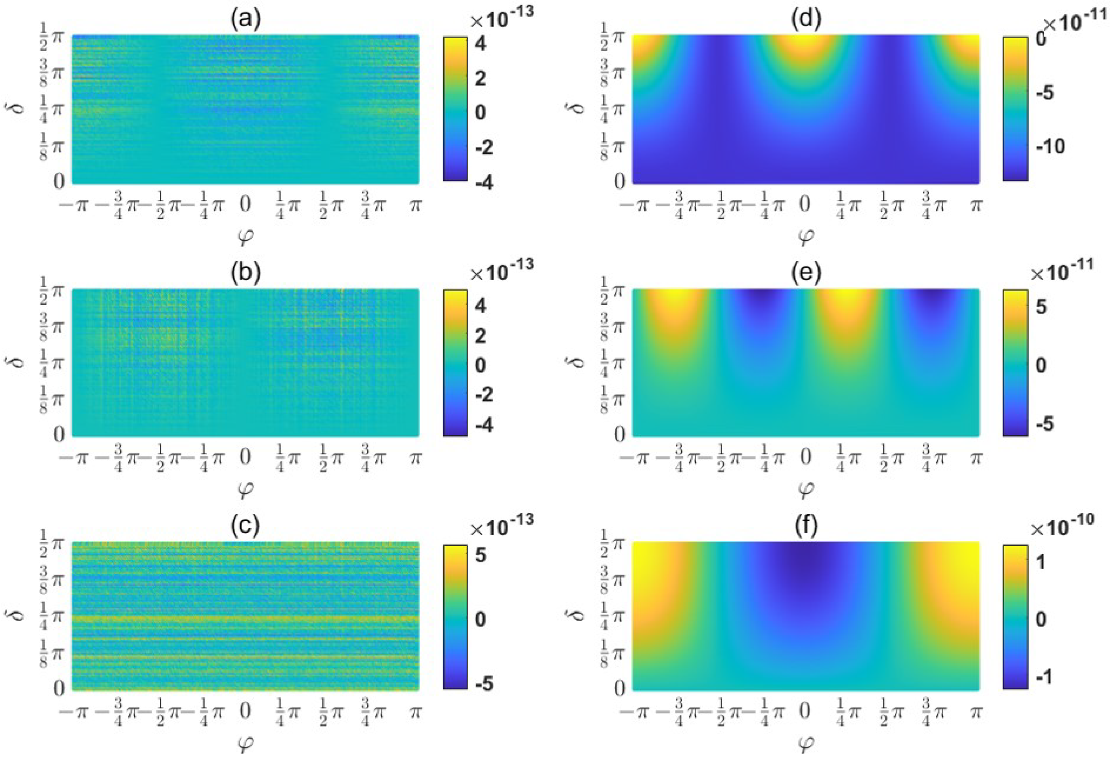
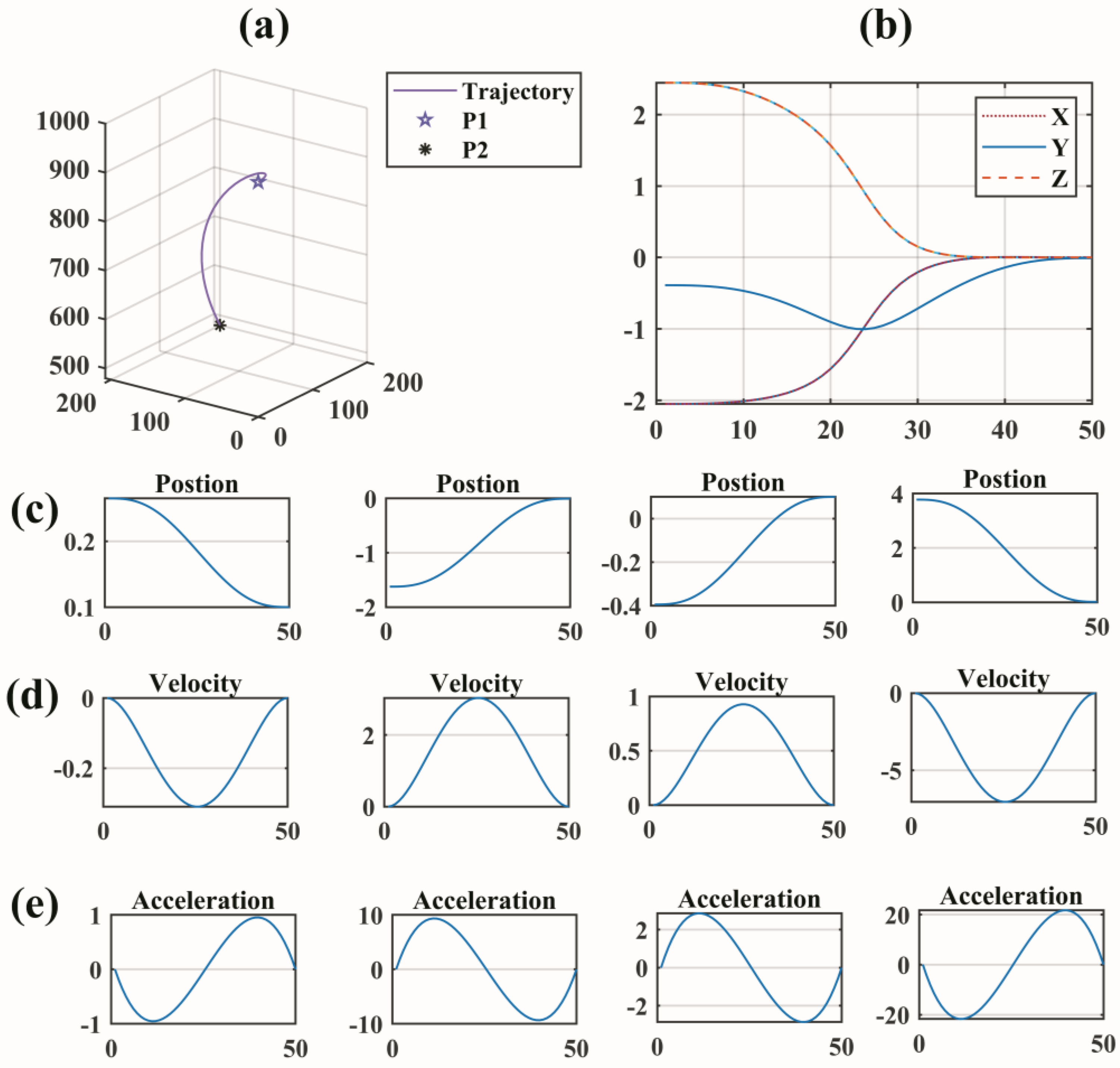
4. Simulation Results and Discussion

To evaluate the accuracy of the dual quaternion model compared to traditional kinematic models, specifically the DH and DH Taylor expansion models, we conducted a comparative analysis using the same driving variable. As demonstrated in Figure 5, our findings reveal that the error computed by the dual quaternion model aligns closely with those of the DH and DH Taylor expansion models. This corroborates the precision and reliability of our proposed methodology. These results underscore the potential of dual quaternions for enhancing the accuracy of kinematic models for continuum robots, laying the groundwork for future research in robotics and related fields. To prove the improvement of calculation speed using dual quaternion modeling, we use the same solution algorithm to solve the same target and compare the calculation time of dual quaternions: DH and DH Taylor. We anticipate the endpoint of the robotic arm to traverse from its initial position, P1 (0, 0, 960 mm), ultimately arriving at the desired position, P2 (369.8146 mm, 345.8315 mm, 702.9017 mm), as shown in Table 1. We used the optimization toolbox in MATLAB, and the CPU was an Intel(R) Xeon(R) W-2245 CPU @ 3.90 GHz 3.91 GHz processor for calculation. From Table 1, we can see that, in the numerical method, the dual quaternion model solves the target position with high precision and a short calculation time of 0.45 s; compared with the traditional DH method of 1.15 s, the calculation time is doubled. In standard meta-heuristic algorithms, the dual quaternion models are shortened by more than half.
To achieve smooth angular velocity and acceleration changes at the end of the robotic arm during operation, a quintic polynomial interpolation algorithm based on dual quaternions is proposed for motion planning of the robotic arm. The simulated movement of the robotic arm end, as illustrated in Figure 6, demonstrates that the velocity and acceleration of the variables are continuum and smooth during the robotic arm’s movement from point P1 to point P2, without any abrupt changes. This indicates that the robotic arm’s motion is not subject to speed distortion and can operate seamlessly.

5. Conclusions

This paper establishes a kinematic model of a continuous robot based on dual quaternions. It derives it from the perspective of the transformation process of geometric elements in space: linear rotation and translation of space. First, the kinematic equations of the line-pulled continuum robot are derived by applying the dual quaternion method. Secondly, the kinematic model of the multi-section complete robotic arm was further established, and the inverse kinematic solution was performed based on the numerical solution method. Finally, this paper proposes a trajectory planning process for a continuum robot using the five-polynomial dual quaternion method.

Author Contributions

Conceptualization, methodology, software, validation, Y.L.; formal analysis, data curation, Q.W.; funding acquisition, Q.L. All authors have read and agreed to the published version of the manuscript.

Funding

This research was funded by Major Science and Technology Project of Hainan Province grant number ZDKJ202006.

Institutional Review Board Statement

Not applicable.

Informed Consent Statement

Not applicable.

Data Availability Statement

Provide data upon reasonable request.

Conflicts of Interest

The authors declare no conflict of interest.

Appendix A

Let there be any two vectors a , b in the space, where the vector a translates the distance l along the p axis, and then rotates θ to become the vector b . Define the dual angle notation, θ ^ = θ + ε l , which relates an arbitrary 3D spatial line a to a given 3D spatial line b by a rotation θ about a unique axis and with a translation l along the same axis.
Here, r a , r b represent the vectors from any arbitrary point in space, denoted as O , to points a and b , respectively. The symbols a , b signify the cross products. The cross products a and b can be represented by a and b and their corresponding r a and r b , as shown in Equation (A1).
Figure A1. Schematic diagram of rotation and translation transformation of a geometric straight line in space.
Applsci 13 11289 g0a1
a = r a × a , b = r b × b
We can write the vectors a and b representing line segments 0 A and 0 B in Plücker form as a ^ and b ^ , respectively.
a ^ = a + ε r a × a , b ^ = b + ε r b × b
Decomposing the vector b along the orthogonal directions of a and p × a gives Equation (A3).
b = cos   θ a + sin   θ p × a
Considering the relationship depicted in the figure, where r b = r a + l , and combining it with the above equation, we can simplify it to Equation (A4).
b ^ = cos   θ ε l sin   θ a + ε r a × a + sin   θ + ε l cos   θ p + ε r a × p × a
The inverse Taylor series transformation is utilized for the change process, as shown in Equation (A5), which ultimately simplifies Equation (A6).
cos   θ ε sin   θ l = cos   θ ^ , sin   θ + ε cos θ l = sin   θ ^
b ^ = cos   θ ^ a ^ + sin   θ ^ p ^ × a ^
Let cos   θ ^ be a dual number, and sin   θ ^ p ^ × a ^ be a dual vector, then applying the concept of dual quaternion, we can see that the elements in coordinate system A are transformed into coordinate system B after a rotation angle θ after a translation distance l around an axis is expressed as Λ ^ = cos   θ ^ + sin θ ^ p ^ , where: b ^ = Λ a ^ . Further, if q ^ a b is equal to the Equation (A7), the b ^ can be expressed as q * ^ a ^ q ^ .
q ^ = cos   θ 2 , sin   θ 2 l + ε d 2 sin   θ 2 , sin   θ 2 m + d 2 cos   θ 2 l

Appendix B

The curvature radius   ρ i j and the center bracket’s curvature radius, which are formed by the changes in each pull line during the driving process, are denoted as R. This is the radius of the circle where the drive line is located. Given that ρ i φ i = l i , ρ i j φ i = l i j , we can calculate ρ i j and l i j according to Equations (A8) and (A9), respectively.
Figure A2. (a) Physical model of a single-section robotic arm in the driving state. (b) Project Plane O E F that drives the rear robotic arm onto plane FZ F X F .
Applsci 13 11289 g0a2
ρ i j = ρ i + R i cos   δ i
l i j = l i + R i φ i cos   δ i j
The cables are evenly distributed in the cross-section of the base, with intervals of 90°. Specifically, we have δ i 1 = δ i ; δ i 2 = δ i + π 2 ; δ i 3 = δ i + π ; δ i 4 = δ i + 3 π 2 . Consequently, the sum of cosine values of i cos δ i j = 0 . Considering the relationship between the main arc length and the four chord lengths, we find that l i = 1 4 i l i j . When the robot joint only undergoes a bending angle δ while the rotation angle is 0, the transformation of the length of the first drive line can be expressed as Equation (A10).
l i 1 = l i l i 1 = ρ i ρ i 1 δ i = ρ i 1 δ i = R i δ i
φ i , θ i and the variation of the four drive l i j when the traction arm bends and twists at the same time. Substitute the rope drives 1 and 2 into l i j = l i + R i φ i cos δ i j to obtain l i 1 = l i + R i φ i cos δ i ; l i 2 = l i R i φ i sin δ i . In the same way, substitute 1 and 3 to obtain l i 1 = l i + R i φ i cos δ i ; l i 3 = l i R i φ i cos δ i . By solving for δ i as shown in Equation (A11), we can determine its value.
δ i = a r c   tan   2 l i 1 l i 2 l i 1 l i 3 1 , δ i π 2 , π 2 , l i R
We can substitute the rope drives 2 and 4 into l i j = l i + R i φ i cos   δ i j to obtain: l i 2 = l i R i φ i sin   δ i ; l i 4 = l i + R i φ i sin   δ i . In the same way, substitute 1, 3 to obtain: l i 1 = l i + R i φ i cos δ i ; l i 3 = l i R i φ i cos δ i . By solving for φ i as shown in Equation (A12), we can determine its value. And because ρ i φ i = l i , l i = 1 4 i l i j , by solving for ρ i as shown in Equation (A13), we can determine its value.
φ i = 1 2 R i l i 4 l i 2 2 + l i 3 l i 1 2
ρ i = R i i l i j 2 l i 4 l i 2 2 + l i 3 l i 1 2

Appendix C

The coordinate system {1} relative to {F} is obtained by rotating the coordinate system along the axis l z 1 by an angle δ .
Then, q F 1 , r = cos   δ 2 , l z 1 sin   δ 2 and q F 1 , d = 1 2 p i q i p i q i * q i , as shown in Equation (A14), the dual quaternion representation.
q ^ F 1 = cos   δ 2   0   0   sin   δ 2   0   0   0   0
The coordinate system {2} is translated relative to coordinate system {1} along the axis l x 1 , given by ρ cos   δ   ρ sin   δ   0 .
We have q 12 , r = 1 , 0 , 0 , 0 T and q 12 , d = 0 , ρ cos   δ , ρ sin   δ , 0 . Thus, the dual quaternion representation q ^ 12 is given by Equation (A15).
q ^ F 1 = cos   δ 2   0   0   sin   δ 2   0   0   0   0
The coordinate system {3} relative to {2} is obtained by rotating the coordinate system along the axis l y 1 by an angle φ .
Then, q 23 , r = cos   φ 2 , l y 1 sin   φ 2 and q 23 , d = 0 , 0 , 0 , ρ sin   φ 2 , as shown in Equation (A16), the dual quaternion representation.
q ^ 23 = cos   φ 2 , sin   δ sin   φ 2 , cos   δ sin   φ 2 , 0 , 0 , 0 , 0 , ρ 2 sin   δ 2 sin   φ 2
The coordinate system {4} is translated relative to coordinate system {3} along the axis l x 3 , given by ρ cos   δ , ρ sin   δ , 0 .
We have q 34 , r = 1 , 0 , 0 , 0 T and q 34 , d = 0 , ρ cos   δ cos   φ , ρ sin   δ sin   φ , ρ sin   φ . Thus, the dual quaternion representation q ^ 34 is given by Equation (A17).
q ^ 34 = 1 , 0 , 0 , 0 , 0 , ρ 2 cos   δ cos   φ , ρ 2 sin   δ cos   φ , ρ 2 sin   φ
The coordinate system { E } relative to {4} is obtained by rotating the coordinate system along the axis l z 4 by an angle δ .
Then, q 4 E , r = cos   δ 2 , l z 4 sin   δ 2 and q 4 E , d = 0 , ρ sin   δ cos   φ 1 sin   δ 2 , ρ cos   δ cos   φ 1 sin   δ 2 , 0 , as shown in Equation (A18), the dual quaternion representation.
q ^ 4 E = cos   δ 2 , cos   δ sin   φ sin   δ 2 , sin   δ sin   φ sin   δ 2 , cos   φ sin   δ 2 , 0 , ρ sin   δ sin   δ 2 cos   φ 1 , ρ cos   δ sin   δ 2 cos   φ 1 , 0
By concatenating the coordinate transformations described in the above equations, we can obtain the transformation dual quaternion between the two coordinate systems, represented as Equation (A19).
q ^ E F = cos   φ 2 , sin   δ sin   φ 2 , cos   δ sin   φ 2 , 0 , 0 , 0 , 0 , ρ sin   φ 2

References

  1. Dou, W.; Zhong, G.; Cao, J.; Shi, Z.; Peng, B.; Jiang, L. Soft Robotic Manipulators: Designs, Actuation, Stiffness Tuning, and Sensing. Adv. Mater. Technol. 2021, 6, 2100018. [Google Scholar] [CrossRef]
  2. Xu, K.; Zhao, J.; Fu, M. Development of the SJTU Unfoldable Robotic System (SURS) for Single Port Laparoscopy. IEEE/ASME Trans. Mechatron. 2015, 20, 2133–2145. [Google Scholar] [CrossRef]
  3. Su, H.; Qi, W.; Schmirander, Y.; Ovur, S.E.; Cai, S.; Xiong, X. A Human Activity-Aware Shared Control Solution for Medical Human–Robot Interaction. Assem. Autom. 2022, 42, 388–394. [Google Scholar] [CrossRef]
  4. Jin, S.; Lee, S.K.; Lee, J.; Han, S. Kinematic Model and Real-Time Path Generator for a Wire-Driven Surgical Robot Arm with Articulated Joint Structure. Appl. Sci. 2019, 9, 4114. [Google Scholar] [CrossRef]
  5. Liu, T.; Mu, Z.; Xu, W.; Yang, T.; You, K.; Fu, H.; Li, Y. Improved Mechanical Design and Simplified Motion Planning of Hybrid Active and Passive Cable-Driven Segmented Manipulator with Coupled Motion. In Proceedings of the 2019 IEEE/RSJ International Conference on Intelligent Robots and Systems (IROS), Macau, China, 3–8 November 2019; pp. 5978–5983. [Google Scholar]
  6. Wang, M.; Dong, X.; Ba, W.; Mohammad, A.; Axinte, D.; Norton, A. Design, Modelling and Validation of a Novel Extra Slender Continuum Robot for in-Situ Inspection and Repair in Aeroengine. Robot. Comput.-Integr. Manuf. 2021, 67, 102054. [Google Scholar] [CrossRef]
  7. Yeshmukhametov, A.; Koganezawa, K.; Yamamoto, Y.; Buribayev, Z.; Mukhtar, Z.; Amirgaliyev, Y. Development of Continuum Robot Arm and Gripper for Harvesting Cherry Tomatoes. Appl. Sci. 2022, 12, 6922. [Google Scholar] [CrossRef]
  8. Xu, F.; Wang, H.; Wang, J.; Au, K.W.S.; Chen, W. Underwater Dynamic Visual Servoing for a Soft Robot Arm with Online Distortion Correction. IEEE/ASME Trans. Mechatron. 2019, 24, 979–989. [Google Scholar] [CrossRef]
  9. Liu, Y.; Ge, Z.; Yang, S.; Walker, I.D.; Ju, Z. Elephant’s Trunk Robot: An Extremely Versatile Under-Actuated Continuum Robot Driven by a Single Motor. J. Mech. Robot. 2019, 11, 051008. [Google Scholar] [CrossRef]
  10. Qin, G.; Ji, A.; Cheng, Y.; Zhao, W.; Pan, H.; Shi, S.; Song, Y. A Snake-Inspired Layer-Driven Continuum Robot. Soft Robot. 2022, 9, 788–797. [Google Scholar] [CrossRef]
  11. Walker, I.D.; Dawson, D.M.; Flash, T.; Grasso, F.W.; Hanlon, R.T.; Hochner, B.; Kier, W.M.; Pagano, C.C.; Rahn, C.D.; Zhang, Q.M. Continuum Robot Arms Inspired by Cephalopods. In Unmanned Ground Vehicle Technology VII; Gerhart, G.R., Shoemaker, C.M., Gage, D.W., Eds.; SPIE: Orlando, FL, USA, 2005; p. 303. [Google Scholar]
  12. Webster, R.J.; Jones, B.A. Design and Kinematic Modeling of Constant Curvature Continuum Robots: A Review. Int. J. Robot. Res. 2010, 29, 1661–1683. [Google Scholar] [CrossRef]
  13. Rucker, D.C.; Webster, R.J., III. Statics and Dynamics of Continuum Robots with General Tendon Routing and External Loading. IEEE Trans. Robot. 2011, 27, 1033–1044. [Google Scholar] [CrossRef]
  14. Till, J.; Aloi, V.; Riojas, K.E.; Anderson, P.L.; Webster Iii, R.J.; Rucker, C. A Dynamic Model for Concentric Tube Robots. IEEE Trans. Robot. 2020, 36, 1704–1718. [Google Scholar] [CrossRef]
  15. Lafmejani, A.S.; Doroudchi, A.; Farivarnejad, H.; He, X.; Aukes, D.; Peet, M.M.; Marvi, H.; Fisher, R.E.; Berman, S. Kinematic Modeling and Trajectory Tracking Control of an Octopus-Inspired Hyper-Redundant Robot. IEEE Robot. Autom. Lett. 2020, 5, 3460–3467. [Google Scholar] [CrossRef]
  16. Amanov, E.; Nguyen, T.D.; Burgner-Kahrs, J. Tendon-Driven Continuum Robots with Extensible Sections—A Model-Based Evaluation of Path-Following Motions. Int. J. Robot. Res. 2019, 40, 027836491988604. [Google Scholar] [CrossRef]
  17. Chitalia, Y.; Deaton, N.J.; Jeong, S.; Rahman, N.; Desai, J.P. Towards FBG-Based Shape Sensing for Micro-Scale and Meso-Scale Continuum Robots with Large Deflection. IEEE Robot. Autom. Lett. 2020, 5, 1712–1719. [Google Scholar] [CrossRef]
  18. Walker, I.D. Continuous Backbone “Continuum” Robot Manipulators. ISRN Robot. 2013, 2013, 726506. [Google Scholar] [CrossRef]
  19. Samadikhoshkho, Z.; Ghorbani, S.; Janabi-Sharifi, F. Coupled Dynamic Modeling and Control of Aerial Continuum Manipulation Systems. Appl. Sci. 2021, 11, 9108. [Google Scholar] [CrossRef]
  20. Sedal, A.; Bruder, D.; Bishop-Moser, J.; Vasudevan, R.; Kota, S. A Continuum Model for Fiber-Reinforced Soft Robot Actuators. J. Mech. Robot. 2018, 10, 024501. [Google Scholar] [CrossRef]
  21. Singh, I.; Amara, Y.; Melingui, A.; Mani Pathak, P.; Merzouki, R. Modeling of Continuum Manipulators Using Pythagorean Hodograph Curves. Soft Robot. 2018, 5, 425–442. [Google Scholar] [CrossRef]
  22. Ma, X.; Chiu, P.W.-Y.; Li, Z. Shape Sensing of Flexible Manipulators with Visual Occlusion Based on Bezier Curve. IEEE Sens. J. 2018, 18, 8133–8142. [Google Scholar] [CrossRef]
  23. Kołota, J.; Kargin, T.C. Comparison of Various Reinforcement Learning Environments in the Context of Continuum Robot Control. Appl. Sci. 2023, 13, 9153. [Google Scholar] [CrossRef]
  24. Godage, I.S.; Walker, I.D. Dual Quaternion Based Modal Kinematics for Multisection Continuum Arms. In Proceedings of the 2015 IEEE International Conference on Robotics and Automation (ICRA), Seattle, WA, USA, 26–30 May 2015; pp. 1416–1422. [Google Scholar]
  25. Araújo, A.L. SMART 2015 7th ECCOMAS Thematic Conference on Smart Structures and Materials, Azores, Portugal, 3–6 June 2015; IDMEC: Lisboa, Portugal, 2015; ISBN 978-989-96276-8-0. [Google Scholar]
  26. Seleem, I.A.; El-Hussieny, H.; Assal, S.F.M.; Ishii, H. Development and Stability Analysis of an Imitation Learning-Based Pose Planning Approach for Multi-Section Continuum Robot. IEEE Access 2020, 8, 99366–99379. [Google Scholar] [CrossRef]
Figure 1. Structure of a continuum tendon-driven robot. (a) Schematic diagram of the robotic arm model in the natural state; (b) Schematic diagram of the robotic arm model in the driven state; (c) Cross-sectional schematic diagram of the robotic arm model. Among them, L i j represents the number of the driving lines, i represents the i th robotic arm, and j represents the j th driving lines.
Applsci 13 11289 g001
Figure 2. The Structure diagram of the single-section mechanical arm is driven and not driven. (a) Schematic diagram of the driving line of the single-section robotic arm when it is not driven, where L i j 0 represents the rope length. (b) Schematic diagram of the driving line of the robotic arm after driving time t, where L i j t represents the rope length.
Applsci 13 11289 g002
Figure 3. (a) Physical model of a single-section robotic arm in the driving state. Among them, {F}{1}{2}{3}{4}{E} are the coordinate systems, respectively, and L E and L F represent the straight lines where the z-axis of the {F} and {E} coordinate systems are located, respectively. (b) Mathematical model of a single-section robotic arm in the driving state. It describes the z-axis and y-axis in the coordinate system {F}, that is, the straight lines L F and P F , which after coordinate transformation become the straight lines L E and P E in the coordinate system {E}.
Applsci 13 11289 g003
Figure 4. The coordinate system of a multi-section continuous robot in a driven state. F i 1 represents the coordinate system at the front end of the continuous robot in the first section, while F i represents it in the second section. Due to physical model limitations, the i -th manipulator’s front-end coordinate system differs from the 1 -section robot arm, but F i and E i 1 remain the same. Thus, a total of i + 1 coordinate systems are needed for the i -section robotic arm.
Applsci 13 11289 g004
Figure 5. The two-section driven manipulator contains four driving variables: φ 1 π , π , δ 1 0 , π / 2 , φ 2 = 0 , and δ 2 0 . The spatial coordinates solved by the DH Taylor expansion series model are used as standard results to compare the errors in the results of the dual quaternion model and the DH model. (a) The dual quaternion model and the standard result solve the error in the x-coordinate direction between the coordinates. (b,c) are the errors in the y-axis and z-axis with the standard result, respectively. (d) The errors between the DH model solution coordinates and the standard result in the x-coordinate direction, (e,f), are the errors on the y-axis and z-axis, respectively.
Applsci 13 11289 g005
Figure 6. Use the fifth-order polynomial interpolation algorithm to plan the trajectory of the robotic arm and solve the problem of the end of the two-section continuous robot moving from point P 1 to point P 2 in space. (a) Schematic diagram of the motion trajectory of the two-section continuous robot. The path is planned through the fifth-order polynomial interpolation algorithm; that is, the continuous robot needs to move 50 steps from point P 1 to point P 2 according to the interpolation sequence. (b) The error between the continuous robot’s actual path and the algorithm’s path (ce), respectively, represents the changes in the angle, angular velocity, and angular acceleration of the driving amount when the continuous robot moves from point P 1 to point P 2 and sequentially moves 50 interpolation trajectory points. The x-axis represents the 50 trajectory points.
Applsci 13 11289 g006
Table 1. Comparison of calculation time and quantity under different models.
ModelOptimization AlgorithmActual PositionIterationsTime(s)
DHGenetic algorithm[369.8147, 345.8322, 702.9025]253.43
Simulated annealing algorithm[369.8150, 345.8317, 702.9021]550062.15
Numerical solution Algorithm[369.8143, 345.8315, 702.9017]321.15
Particle Swarm Optimization[369.8125, 345.8306, 702.9003]2253.36
DH Taylor expansionGenetic algorithm[372.2827, 347.7579, 706.3873]4004.50
Simulated annealing algorithm[369.8165, 345.8329, 702.9044]770052.30
Numerical solution Algorithm[369.8146, 345.8319, 702.9018]310.41
Particle Swarm Optimization[369.8101, 345.8311, 702.8985]3804.60
dual quaternionsGenetic algorithm[369.8161, 345.8352, 702.9070]3502.39
Simulated annealing algorithm[369.8118, 345.8293, 702.8986]390028.50
Numerical solution Algorithm[369.8146, 345.8319, 702.9018]320.45
Particle Swarm Optimization[366.5362, 345.7464, 701.7661]851.18
Disclaimer/Publisher’s Note: The statements, opinions and data contained in all publications are solely those of the individual author(s) and contributor(s) and not of MDPI and/or the editor(s). MDPI and/or the editor(s) disclaim responsibility for any injury to people or property resulting from any ideas, methods, instructions or products referred to in the content.

