Stress Intensity Factors for Pressurized Pipes with an Internal Crack: The Prediction Model Based on an Artificial Neural Network

Abstract

During pipeline operation, internal cracks may occur. The severity around the crack tip can be quantified by the stress intensity factor (K_I), which is a linear–elastic fracture mechanics parameter. For pressurized pipes featuring infinitely long internal surface cracks, K_I can be interpolated from a function considering pressure, geometry, and crack size, as presented in API 579-1/ASME FFS-1. To enhance K_I prediction accuracy, an artificial neural network (ANN) model was developed for such pressurized pipes. Predictions from the ANN model and API 579-1/ASME FFS-1 were compared with precise finite element analysis (FEA). The ANN model with an eight-neuron sub-layer outperformed others, displaying the lowest mean squared error (MSE) and minimal validation discrepancies. Nonlinear validation data improved both MSE and testing performance compared to uniform validation. The ANN model accurately predicted normalized K_I, with differences of 2.2% or lower when compared to FEA results. Conversely, API 579-1/ASME FFS-1′s bilinear interpolation predicted inaccurately, exhibiting disparities of up to 4.3% within the linear zone and 24% within the nonlinearity zone. Additionally, the ANN model effectively forecasted the critical crack size (a_C), differing by 0.59% from FEA, while API 579-1/ASME FFS-1′s bilinear interpolation underestimated a_C by 4.13%. In summary, the developed ANN model offers accurate forecasts of normalized K_I and critical crack size for pressurized pipes, providing valuable insights for structural assessments in critical engineering applications.

1. Introduction

During the operation of a pipeline, various types of flaws can occur, including volumetric flaws (e.g., pores, inclusions, undercuts, and overlaps) as well as crack-like flaws characterized by planar flaws with a sharp root radius [1,2]. According to the recommendations outlined in API 579-1/ASME FFS-1 [3], it is advisable to treat volumetric flaws in the close vicinity as crack-like flaws, the severity of which could be characterized by length and depth. A crack-like flaw intends to create an idealized crack geometry that is intentionally conservative (i.e., more severe than the actual volumetric flaws).

Under the combination of mechanical action and environment, the propagation of a surface crack is possible and becomes a serious risk to the structural integrity of the pipeline system. The severity of a crack can be quantified by a linear–elastic fracture mechanics parameter, known as the stress intensity factor or K [4]. If K is higher than the fracture toughness of pipe material (i.e., the critical stress intensity factor or K_C), the crack propagates rapidly, and a sudden fracture of the pipeline is possible. On the other hand, if K is lower than K_C but still high enough to initiate crack propagation, the crack could propagate in the thickness of the pipe (i.e., a propagating crack), eventually leading to leakage (i.e., a through-thickness crack). With periodic observation and life assessment, the service of a cracked pipeline may be allowed to continue until appropriate maintenance is performed [2]. For a pipe under internal pressure, the semi-elliptical crack-like flaws are likely to nucleate at an inner wall and in the longitudinal direction due to the influence of hoop stress [5]. Because the K under opening mode (i.e., K_I) at the deepest point of an infinitely long crack could be considered the upper limit of K_I for the pressurized pipe with semi-elliptical surface cracks [3,6]; the K_I solution for an infinitely long crack is recommended by API 579-1/ASME FFS-1 for a cracked pipe under internal pressure.

For a pressurized pipe with an infinitely long internal surface crack in the longitudinal direction, K_I can be numerically calculated using finite element analysis (FEA). However, the FEA for an accurate K_I requires various resources, such as numerical skills, computational hardware, and time. As an alternative, the K_I values obtained from FEA are mathematically arranged into a simple function based on applied pressure, geometry, and crack size, as presented in API 579-1/ASME FFS-1. Interpolations are necessary to obtain the required geometry function when the geometry of a cracked pipe does not exactly match those provided in API 579-1/ASME FFS-1. Although the geometry functions for various crack sizes and pipe thicknesses are nonlinear, linear interpolation is typically employed for the required geometry function. Rahman et al. [7] found that for shallow cracks in a pipe, linear interpolation does not yield a significant difference in K_I when compared with nonlinear interpolation. However, for deep cracks in a pipe, the difference becomes more pronounced (i.e., up to 6%).

As an intelligence created by machines to solve complex problems, artificial intelligence (AI) has successfully been applied in various engineering domains. These applications include predicting the compressive strength of concrete [8], determining the stiffness matrix of functionally-graded nanoplates [9], generating performance data for a steam methane reformer (SMR) [10], forecasting electric energy consumption [11], analyzing fuel efficiency for cargo vessel operation [12], and identifying damages in components as well as determining the fracture toughness of materials [13,14]. Among various AI methods, the artificial neural network (ANN) method [15] simulates a brain by using artificial neurons that transmit and process signals between each other. The signal at a connection of artificial neurons is a real number, and the output of each artificial neuron is computed by a nonlinear function. During the training process, the weights and biases of artificial neurons are repetitively adjusted based on the difference between the processed output (i.e., the prediction) and the target output (i.e., the known solution). The training continues until a sufficient number of these adjustments are made, and subsequently, the ANN model is applied to solve the actual problems.

The applications of ANN for predicting fracture toughness include studies by Wiangkham et al. [16] on polymethyl methacrylate (PMMA), Hamdia et al. [17] on polymer nanocomposites (PNCs), Guha Roy et al. [18] on rocks, and Liu et al. [19] on Nb-Si alloys. On the other hand, the applications of ANN for predicting stress intensity factors include studies by Muñoz-Abella et al. [20] on unbalanced rotating cracked shafts, Wu et al. [21] on cracked pavements under traffic loading, and Li et al. [22] on through-thickness cracks in bending tubes. Although ANN has been previously applied for predicting stress intensity factors in cracked tubes [22], it was specifically designed only for through-thickness cracks. However, the application of ANN for predicting stress intensity factors of propagating cracks in pipes (which require periodic observation and life assessment to prevent crack propagation through the thickness of the pipe) has not been investigated yet.

Due to the complexity of FEA, the impact of linear interpolation on the accuracy of the geometry function from API 579-1/ASME FFS-1, and the absence of an ANN model for predicting stress intensity factors of propagating cracks in pipes, it is the objective of this work to investigate the applicability of the ANN model for predicting K_I in a pressurized pipe with an infinitely long internal surface crack in the longitudinal direction. The ANN model consists of two input factors: the ratio between crack size and pipe thickness (a/t) and the ratio between pipe thickness and internal radius (t/R_i), and an output factor being K_I. The K_I solutions from API 579-1/ASME FFS-1 were used for training, while those from FEA were used for validation. Subsequently, the ANN model was applied to predict K_I for actual problems, involving cracked pipes with geometry different from those provided in API 579-1/ASME FFS-1. The predicted K_I values were compared with the FEA solutions for accuracy assessment. The applicability of the ANN model for predicting K_I in a pressurized pipe with an infinitely long internal surface crack in the longitudinal direction was then discussed.

2. Research Method

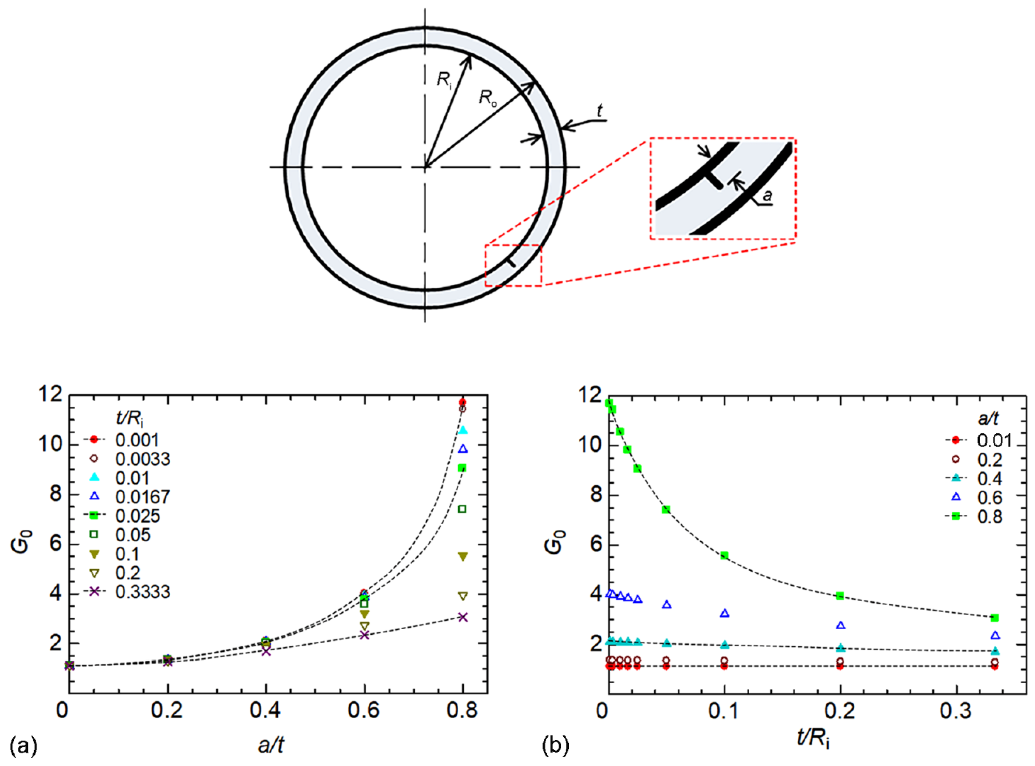
2.1. Stress Intensity Factor from API 579-1/ASME FFS-1

For a homogeneous and linear-elastic engineering component, K_I depends on the geometry of the component (i.e., the geometry, size and location of the crack) and the applied mechanical action (i.e., type and magnitude of applied load) [4]. As an example, K_I for an infinite plate with a single-edge crack can be written as follows:

$$K_{\mathrm{I}}=\sigma \sqrt{\pi a}f\left(\alpha \right),$$

(1)

$$f\left(\alpha \right)=0.265{\left(1-\alpha \right)}^4+\frac{0.857+0.265\alpha }{{\left(1-\alpha \right)}^{3/2}},$$

(2)

$$\alpha =\frac{a}{W},$$

(3)

where σ is the applied stress, a is the crack size, W is the plate width, and f(a/W) is the geometry function.

For the pressurized pipe with an infinitely long internal surface crack in the longitudinal direction (Figure 1), K_I can be calculated using the formula provided in API 579-1/ASME FFS-1:

$$K_{\mathrm{I}}=\frac{P{R}_{\mathrm{o}}^2}{R_{\mathrm{o}}^2-R_{\mathrm{i}}^2}\sqrt{\pi a}\left[2G_0-2G_1\left(\frac{a}{R_{\mathrm{i}}}\right)+3G_2{\left(\frac{a}{R_{\mathrm{i}}}\right)}^2-4G_3{\left(\frac{a}{R_{\mathrm{i}}}\right)}^3+5G_4{\left(\frac{a}{R_{\mathrm{i}}}\right)}^4\right],$$

(4)

where P is the internal pressure, a is the crack size, R_i is the internal radius, R_o is the external radius, and G₀ to G₄ are the influence coefficients. API 579-1/ASME FFS-1 provides influence coefficients that cover the range of 0.01 ≤ a/t ≤ 0.8 and 0.001 ≤ t/R_i ≤ 0.3333. As an example of the nonlinear behavior of the influence coefficient, the variation of G₀ with respect to a/t and t/R_i is shown in Figure 1a,b, respectively.

For the a/t and t/R_i of cracked pipes, which do not exactly correspond to those provide in API 579-1/ASME FFS-1, linear interpolation is usually applied to estimate the required influence coefficients. The linear interpolation for the unknown function f(x) can be expressed as follows:

$$f\left(x\right)=f\left(x_0\right)+\left(x-x_0\right)\frac{f\left(x_1\right)-f\left(x_0\right)}{x_1-x_0},$$

(5)

where x, x₀, and x₁ are the input parameters (i.e., x is between x₀ and x₁) and f(x₀) and f(x₁) are the known functions. According to the nonlinear behavior of the influence coefficients, it is likely that the interpolated influence coefficients and subsequently estimated K_I could be inaccurate.

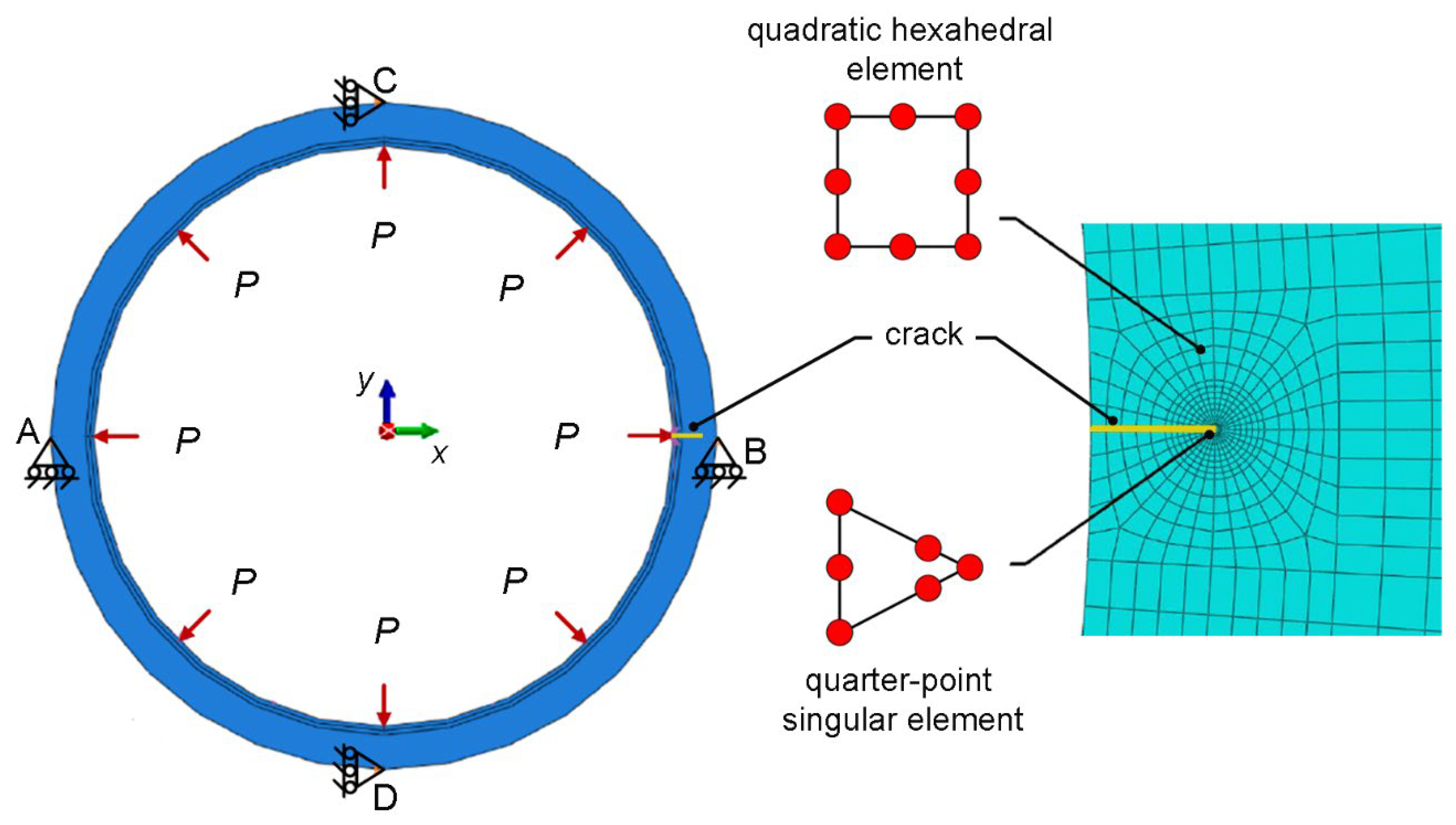
2.2. FEA of Stress Intensity Factor

A two-dimensional linear-elastic plane-strain FEA of the pressurized pipe with an infinitely long internal surface crack in the longitudinal direction was performed using a commercial FEA software (ABAQUS 2016 [23]). The FE model of the cracked pipe is shown in Figure 2. The elements around the crack tip were quarter-point singular elements, while quadratic hexahedral elements were used elsewhere. Both the quarter-point singular element and the quadratic hexahedral element can be considered as the eight-node biquadratic plane strain element, which employs quadratic interpolation functions and incorporates reduced integration techniques for computational efficiency (i.e., CPE8R [23]). Regarding the boundary conditions, the displacements at location A and B were allowed only in the x direction, while those at location C and D were allowed only in the y direction. The pipe material was assumed to be steel with an elastic modulus (E) of 210 GPa and a Poisson’s ratio (ν) of 0.3.

During the FEA, the internal pressure (P) was gradually increased in 20 steps from zero to the maximum pressure, and the K_I at the crack tip was calculated. To minimize the dependence of the FEA results on the element size, the element size was varied until the K_I became stable, indicated by a variation in K_I lower than 3%. The FEA model consisted of 15,692 elements and 48,260 nodes, and the smallest element at the crack tip measured 100 μm.

To validate the FE model, the cracked pipe with a R_i of 100 mm and P of 1 MPa was analyzed. Using various a/t and t/R_i ratios, the K_I values obtained from the FEA were compared with the values estimated from API 579-1/ASME FFS-1, as shown in Figure 3. The K_I values obtained from the FEA are in good agreement with those from API 579-1/ASME FFS-1, with maximum differences lower than 2%. As a result, the validated FE model was utilized to calculate the K_I for cracked pipes with geometries different from those described in API 579-1/ASME FFS-1.

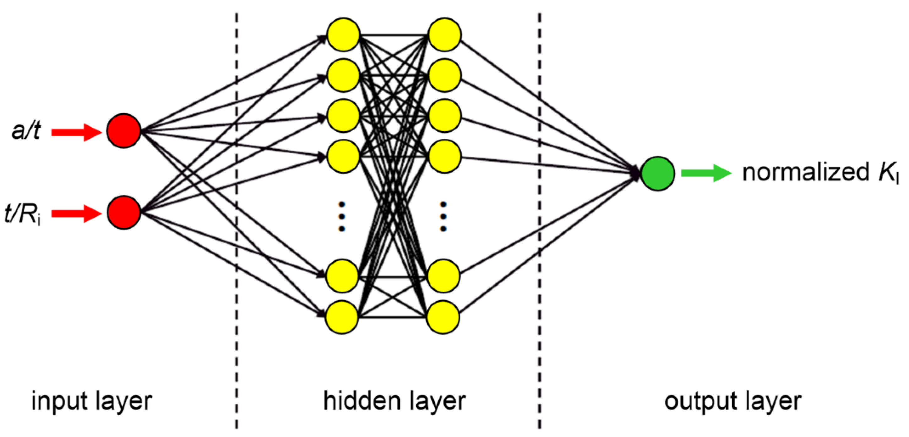
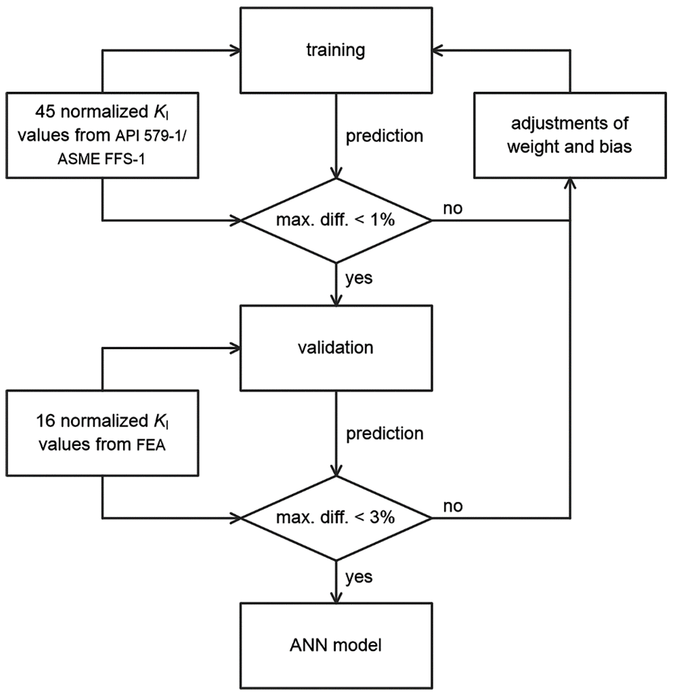
2.3. ANN Model for the Prediction of Stress Intensity Factor

For various values of a/t and t/R_i, the K_I values obtained from API 579-1/ASME FFS-1 were normalized using the applied pressure, pipe geometry, and crack size, as follows:

$$K_{\mathrm{I}}\frac{R_{\mathrm{o}}^2-R_{\mathrm{i}}^2}{P{R}_{\mathrm{o}}^2\sqrt{\pi a}}=2G_0-2G_1\left(\frac{a}{R_{\mathrm{i}}}\right)+3G_2{\left(\frac{a}{R_{\mathrm{i}}}\right)}^2-4G_3{\left(\frac{a}{R_{\mathrm{i}}}\right)}^3+5G_4{\left(\frac{a}{R_{\mathrm{i}}}\right)}^4,$$

(6)

This normalized value, also referred to as the geometry function (F), was used during the formation of the ANN model. The normalized K_I for a/t and t/R_i obtained from API 579-1/ASME FFS-1 are shown in Figure 4.

The ANN model was constructed using a commercial software, i.e., MATLAB: Neural Network Toolbox 7 [24]. The structure of the ANN model (Figure 5) consists of the following components: (i) an input layer with two neurons representing a/t and t/R_i, (ii) a hidden layer with two sub-layers, and (iii) an output layer with one neuron representing normalized K_I. The Tan-Sigmoid activation function, mathematically represented by the equation:

$$f\left(x\right)=\frac{2}{1+e^{-2x}}-1,$$

(7)

was chosen for the signal at the connection of artificial neurons in the hidden layer. In this equation, x represents the sum of weights.

A schematic diagram illustrating the training and validation process is shown in Figure 6. The 45 normalized K_I values obtained from API 579-1/ASME FFS-1 were used as training data. After training, the ANN model was employed to predict the training data, and the difference between each predicted output and its corresponding actual training data was calculated. As the parameter represents the least accurate prediction, the maximum difference between the actual training data and the prediction was used to evaluate the prediction performance. If the maximum difference was higher than 1%, the weights and biases on the hidden layer of the ANN model were adjusted before another iteration of training. On the other hand, if the maximum difference was lower than 1%, the ANN model was subsequently used to predict the validation data (i.e., 16 normalized K_I values obtained from FEA). It is noted that the a/t and t/R_i values of the validation data were different from those of the training data, and the ratio between the training data and validation data was approximately 3:1. During the validation, if the maximum difference between the predicted output and the validation data was higher than 3%, the weights and biases on the hidden layer of the ANN model were adjusted before another iteration of training and validation. This method of weight and bias adjustments is called the “backpropagation method”. The training and validation process continued until the maximum difference between the predicted output and the validation data became lower than 3%.

As an essential part of the training and validation process, the adjustments of weight and bias allow the network to learn and improve its accuracy in making predictions. The weight adjustment of artificial neurons in the hidden layer is performed using the Levenberg–Marquardt backpropagation (LM) training function, as follows [24]:

$$w_{k+1}=w_k-{\left(J_k^{\mathrm{T}}{J}_k+\mu I\right)}^{-1}{J}_k{e}_k,$$

(8)

where w is the weight, k is the index of the iteration, J is the Jacobian matrix, J^T is the Hessian matrix obtained from the Jacobian matrix, e is the training error between the network output and the reference output at iteration k, I is the identity matrix, and μ is the combination coefficient. Similar to the weight adjustment, the bias adjustment of artificial neurons in the hidden layer also uses the Levenberg–Marquardt backpropagation (LM) training function. Further information about the formulation of the ANN model, in addition to what is described in Figure 6, is available in ref. [15,24].

The number of neurons in each sub-layer of the hidden layer was determined through a trial-and-error approach. Based on a previous investigation [16], a sub-layer with 10 neurons was initially selected, and then the training and validation processes were applied to the ANN model. The validation data (i.e., the normalized K_I obtained from the FEA) were uniformly selected among the training data. The predicted output and the validation data were compared, and their differences were calculated. To determine the appropriate number of neurons in each sub-layer of the ANN model, the number of neurons was adjusted between 6 to 12 neurons, and the number of neurons that corresponded to the ANN model with the smallest difference between the predicted output and the validation data was chosen.

Because validation helps determine the ability of the ANN model to predict beyond the training data (i.e., unseen data) and provides an indication for the improvement of the ANN model via the adjustments of weight and bias, the selection of validation data may affect the performance of the ANN model. Accordingly, two models of validation data were investigated in the present work: model A involves uniformly selecting validation data among the training data, while model B selects validation data based on the nonlinearity of the training data. In model B, more validation data were chosen from the nonlinearity zone compared to the linearity zone of the training data.

Based on the coefficient of determination (R²), the linearity and nonlinearity of the training data in the functions of a/t and t/R_i were analyzed, i.e., linear behavior (R² ≥ 0.95) and nonlinear behavior (R² < 0.95). Schematic diagrams showing the training data and validation data for model A and model B are presented in Figure 7a,b, respectively. In model B, since the normalized K_I values exhibited nonlinear behavior for pipes with deep cracks (0.4 < a/t ≤ 0.8) and thin walls (0.001 ≤ t/R_i < 0.1), nine validation data points were selected from the nonlinear ranges of the training data, while seven validation data points were selected from the linear ranges of the training data. Conversely, in model A, regardless of the nonlinearity exhibited by the training data, 16 validation data points were uniformly chosen among the training data, whereas only four validation data points were selected from the ranges of nonlinear training data.

In order to assess the suitability of the ANN model in predicting K_I for a pressurized pipe with an infinitely long internal surface crack in the longitudinal direction (referred to as “testing”), the ANN models A and B were applied to predict 25 normalized K_I values. These testing scenarios involved cracked pipes with geometries distinct from those outlined in API 579-1/ASME FFS-1 and those previously employed in the validation (Figure 7a,b). The predicted values were subsequently compared with the normalized K_I values obtained from FEA. The applicability of the ANN model for predicting K_I in a pressurized pipe with an infinitely long internal surface crack in the longitudinal direction was then discussed.

3. Results and Discussion

3.1. Influence of Number of Neurons in Sub-Layer on the Performance of ANN Model

As a common parameter used to quantify the average squared difference between predicted values and actual values in a dataset, the mean squared error (MSE) was applied to evaluate the influence of the number of neurons in a sub-layer on the performance of the ANN model. A lower MSE value indicates that the predictions of the ANN model are closer to the actual values. For example, the reduction in MSE with the epochs (i.e., the iterations of training and validation) of ANN model A with eight neurons is shown in Figure 8. Initially, the weights and biases of the training data were randomly selected, and the MSEs were calculated. Subsequently, the weights and biases were adjusted before the next epoch. The MSE of the ANN model improved with each epoch and eventually converged, indicating that further improvements in the model’s performance are unlikely.

To evaluate the influence of the number of neurons in a sub-layer on the performance of the ANN model, the converged MSE and maximum difference of ANN model A with 6 to 12 neurons were calculated and compared, as listed in

Table 1. Influence of number of neurons in sub-layer on the performance of ANN model.

Number of Neurons	MSE		Maximum Difference (%)
	Training Data	Validation Data	Training Data	Validation Data
6	0.00034	0.10270	0.77	5.81
7	0.00037	0.07500	0.58	5.07
8	0.00002	0.00510	0.53	2.04
9	0.00013	0.01580	0.25	6.70
10	0.00024	0.01810	0.35	9.14
11	0.00036	0.02780	0.46	11.65
12	0.00021	0.05700	0.32	13.40

. It is observed that the ANN model with eight neurons provides the lowest MSE and the smallest maximum difference in validation data, i.e., 0.00510 and 2.04%, respectively. Therefore, eight neurons in the sub-layer was the appropriate number for the present ANN model.

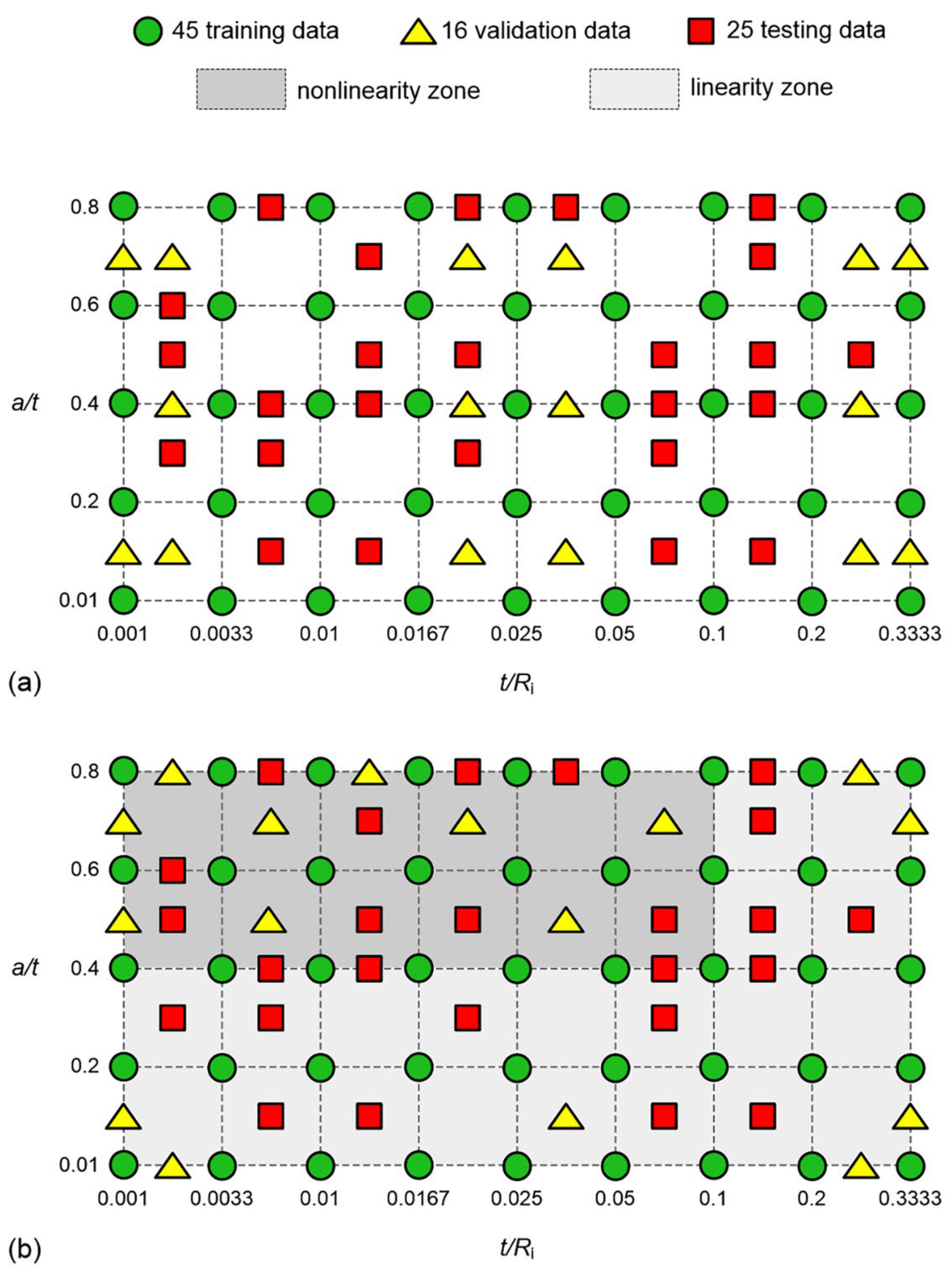
3.2. Influence of Validation Data on the Performance of ANN Model

To evaluate the influence of validation data on the performance of the ANN model with eight neurons, the MSE and maximum difference of ANN models A and B were calculated and compared, as listed in

Table 2. Influence of validation data on the performance of ANN model.

ANN Model	MSE			Maximum Difference (%)
	Training Data	Validation Data	Testing Data	Training Data	Validation Data	Testing Data
A	0.00002	0.00510	0.00513	0.53	2.04	3.97
B	0.00022	0.01040	0.00309	0.40	2.44	2.16

. As depicted in Figure 7, the validation data for model B were mainly selected from the nonlinear ranges of the training data (consisting of nine validation data points), whereas the validation data for model A were mainly selected from the linear ranges of the training data (consisting of 12 validation data points). Since predicting the linear behavior of validation data is easier, model A exhibits a lower MSE and a smaller maximum difference in validation data, i.e., 0.00510 and 2.04%, respectively.

On the other hand, when both models were applied to predict 25 testing data points (i.e., randomly selected as illustrated in Figure 7), model B yielded a lower MSE and a smaller maximum difference in testing data, i.e., 0.00309 and 2.16%, respectively. This suggests that selecting nonlinear validation data (as performed in model B) enhances the performance of the ANN model in predicting testing data. Consequently, model B is considered as appropriate choice for predicting the K_I of a pressurized pipe with an infinitely long internal surface crack in the longitudinal direction.

3.3. Comparison between the Normalized K_I from API 579-1/ASME FFS-1 and ANN Model

The cracked pipes, requiring the interpolation of normalized K_I from API 579-1/ASME FFS-1, were divided into two groups: the linear interpolation (Lerp) group and the bilinear interpolation (BiLerp) group. In the Lerp group, pipes with t/R_i values not matching those provided in API 579-1/ASME FFS-1 were selected. Since the a/t ratios of the selection corresponded to those in API 579-1/ASME FFS-1, Lerp was utilized to estimate normalized K_I values between two t/R_i points. On the other hand, in the BiLerp group, the cracked pipes with a/t and t/R_i values not exactly corresponding to those in API 579-1/ASME FFS-1 were chosen. As a result, BiLerp was employed to estimate normalized K_I values between two a/t points and two t/R_i points. The normalized K_I values of the Lerp and BiLerp groups were also estimated using an ANN model. Subsequently, the predictions of normalized K_I from both API 579-1/ASME FFS-1 and the ANN model were compared with those obtained from FEA, which represents the accurate solution for K_I.

The normalized K_I values obtained from the Lerp of API 579-1/ASME FFS-1 and the ANN model were compared to those obtained from FEA, as listed in

Table 3. Comparison between the predictions of normalized K_I from the linear interpolation of API 579-1/ASME FFS-1 and the ANN model.

Zone	Testing Data		Normalized KI			Difference (%)
	t/Ri	a/t	FEA	ANN	Lerp	ANN vs. FEA	Lerp vs. FEA
linearity zone	0.002	0.4	4.2120	4.2022	4.2052	−0.23	−0.16
	0.15	0.4	3.6844	3.7103	3.6821	0.70	−0.06
	0.25	0.4	3.3961	3.3419	3.3976	−1.60	0.04
nonlinearity zone	0.002	0.6	8.0180	8.0103	8.0101	−0.10	−0.10
	0.006	0.6	7.9288	7.9085	7.9087	−0.26	−0.25
	0.006	0.8	22.1026	22.0536	22.1218	−0.22	0.09
	0.012	0.6	7.7972	7.7747	7.7838	−0.29	−0.17
	0.02	0.6	7.6293	7.6160	7.6130	−0.17	−0.21
	0.02	0.8	18.9014	18.8772	18.9039	−0.13	0.01
	0.04	0.8	15.7327	15.7047	15.9116	−0.18	1.14

. The normalized K_I values obtained from the Lerp of API 579-1/ASME FFS-1 and the ANN model exhibit strong agreement with the FEA results. The differences in normalized K_I within the linearity and nonlinearity zones are both less than 1.6%. This confirms the suitability of both the Lerp of API 579-1/ASME FFS-1 and the ANN model for predicting K_I in pressurized pipes with infinitely long internal surface cracks in the longitudinal direction.

For the BiLerp group, the normalized K_I values obtained from the BiLerp of API 579-1/ASME FFS-1 and the ANN model were compared to those obtained from FEA, as listed in

Table 4. Comparison between the predictions of normalized K_I from the bilinear interpolation of API 579-1/ASME FFS-1 and the ANN model.

Zone	Testing Data		Normalized KI			Difference (%)
	t/Ri	a/t	FEA	ANN	BiLerp	ANN vs. FEA	BiLerp vs. FEA
linearity zone	0.002	0.1	2.3657	2.4114	2.4676	1.93	4.31
	0.02	0.1	2.3717	2.4074	2.4578	1.51	3.63
	0.25	0.1	2.2993	2.3358	2.3715	1.59	3.14
nonlinearity zone	0.002	0.5	5.6197	5.5627	6.1076	0.59	8.68
	0.002	0.7	12.5583	12.6429	15.5746	0.67	24.02
	0.012	0.5	5.5399	5.5885	5.9715	0.88	7.79
	0.012	0.7	11.9121	11.7481	14.1883	−1.38	19.11
	0.02	0.5	5.4693	5.5277	5.8699	1.07	7.33
	0.04	0.7	10.3687	10.1446	11.5745	−2.16	11.63
	0.075	0.5	5.0328	5.0686	5.2976	0.71	5.26

. The BiLerp of API 579-1/ASME FFS-1 fails to accurately predict the normalized K_I values, leading to differences of up to 4.3% within the linearity zone and up to 24% within the nonlinearity zone. However, the ANN model continues to successfully predict the normalized K_I values, with differences within the linearity and nonlinearity zones both remaining below 2.2%. This reaffirms the applicability of the ANN model for predicting K_I in pressurized pipes with infinitely long internal surface cracks in the longitudinal direction.

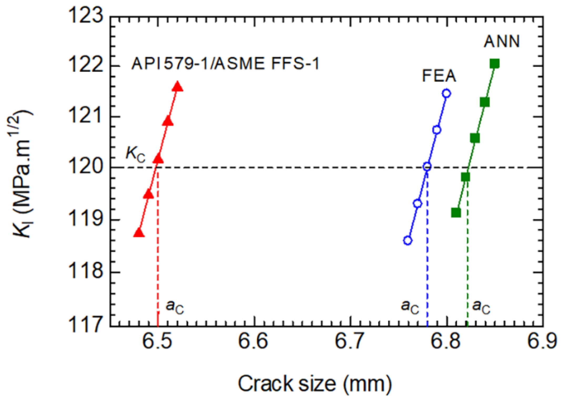
3.4. Application of ANN Model for the Estimation of Critical Crack Size of a Pipe

In fracture mechanics, the critical crack size (a_C) is the maximum size of a crack that an engineering component can tolerate without failing. The a_C is a vital consideration in engineering design and structural integrity assessments. Engineers need to ensure that critical crack sizes are adequately controlled and do not reach unsafe levels that could lead to catastrophic failures. To estimate the critical crack size (a_C), the K_I at the crack tip is determined. If the K_I is higher than the fracture toughness of the material (K_C), the crack propagates rapidly, and a sudden fracture of an engineering component is possible [4].

As a case study, the a_C of a 304 stainless steel cracked pipe with a t/R_i of 0.012, a thickness of 9.5 mm, and subjected to an internal pressure of 1.5 MPa [25] was estimated using FEA, API 579-1/ASME FFS-1, and ANN. The relationships between K_I and a obtained from FEA, API 579-1/ASME FFS-1, and ANN are shown in Figure 9. It is observed that K_I increases with a. To identify the a_C, the fracture toughness (K_C) of 304 stainless steel (i.e., 120 MPa.m^1/2 [26]) is indicated in the figure. At the point where the calculated K_I equaled the K_C value, the corresponding crack size was determined as the a_C. The a_C values obtained from FEA, API 579-1/ASME FFS-1, and ANN are 6.78, 6.50, and 6.82 mm, respectively.

The BiLerp prediction from API 579-1/ASME FFS-1 fails to accurately predict the a_C, being approximately 4.13% lower than the a_C obtained from FEA. However, the ANN model continues to successfully predict the a_C, with a difference of approximately 0.59% higher than the a_C obtained from FEA. The lower BiLerp prediction of a_C compared to the accurate prediction from FEA may lead to premature replacement of cracked pipes, resulting in increased costs. Moreover, for improving the fracture resistance of pipes and selecting optimal operating conditions, accurate a_C values are essential. This reaffirms the applicability of the present ANN model for predicting both K_I and a_C in pressurized pipes with infinitely long internal surface cracks in the longitudinal direction.

3.5. Discussion

Based on 45 training data and 16 validation data, the current ANN model with eight neurons in a sub-layer successfully predicted the normalized K_I values and a_C for a pressurized pipe with an infinitely long internal surface crack in the longitudinal direction. The differences from FEA results were lower than 2.2% and higher than 0.59% for normalized K_I values and a_C, respectively. It is understood that the performance of the ANN model depends on various parameters, with the impact of the number of training data and validation data being considered one of the most significant [15]. If additional training data and validation data are utilized in the construction of the ANN model, an enhancement in the model’s performance can be expected.

The influences of interpolation methods (i.e., linear and nonlinear interpolations) on the estimated K_I in pressurized pipes with infinitely long internal surface cracks in the longitudinal direction have been investigated by Seenuan et al. [27]. They found that cubic spline interpolation (i.e., a mathematical technique that uses piecewise cubic polynomials to create a continuous curve representing a set of discrete data points) can offer a better prediction of normalized K_I from API 579-1/ASME FFS-1 when compared to linear interpolation and other nonlinear interpolations. However, the normalized K_I values estimated by cubic spline interpolation was still significantly different from those obtained from FEA, i.e., the maximum difference was up to 7.3% within the nonlinearity zone. Given its lower accuracy compared to the estimation using the present ANN model, it would be more appropriate to estimate the K_I in pressurized pipes with infinitely long internal surface cracks in the longitudinal direction using the ANN model.

As the main practical applications of this work, the ANN model can be applied for predicting K_I in a pressurized pipe with an infinitely long internal surface crack in the longitudinal direction. Because the severity of a crack was quantified by K_I, the ANN model can be applied to any pipes made of linear-elastic materials. In addition to the cases presently investigated, determining the normalized K_I values and a_C for pipes exhibiting alternative crack shapes (e.g., circumferential cracks, inclined cracks, free cracks), diverse pipe geometries (e.g., elbow pipes, T-shape pipes), and/or varied mechanical loading scenarios (e.g., bending, tension, torsion) presents significantly greater complexity. Generally, the normalized K_I values and a_C for these problems can be numerically calculated using FEA. However, FEA demands advanced numerical skills and prolonged computational time. Consequently, the application of ANN could yield benefits in estimating the normalized K_I values and a_C for these complex problems. As a result, further investigation is imperative for guiding future research in this field.

4. Conclusions

In this study, an artificial neural network (ANN) model was developed and employed to predict the normalized stress intensity factor (K_I) for a pressurized pipe with an infinitely long internal surface crack in the longitudinal direction. The predictions of normalized K_I from both API 579-1/ASME FFS-1 and the ANN model were compared with those obtained from the finite element analysis (FEA), which provides an accurate solution for normalized K_I. The key findings related to the ANN model formulation are as follows:

• Among the ANN models with 6 to 12 neurons in a sub-layer, the model with 8 neurons exhibited the lowest mean squared error (MSE) and the smallest maximum difference in validation data. Therefore, the suitable number of neurons for the present ANN model was determined to be eight in the sub-layer.
• The ANN model that selected nonlinear validation data demonstrated a lower MSE and a smaller maximum difference in testing data compared to uniformly selecting validation data among the training data. This observation suggested that choosing nonlinear validation data improved the performance of the ANN model.
• Regarding the performance of the ANN model:
• The ANN model successfully predicted normalized K_I values, with differences from FEA results lower than 2.2%. Thus, the applicability of the ANN model for predicting K_I in pressurized pipes with infinitely long internal surface cracks in the longitudinal direction was confirmed. On the other hand, the bilinear interpolation (BiLerp) of API 579-1/ASME FFS-1 failed to accurately predict normalized K_I values, resulting in differences up to 4.3% within the linear zone and up to 24% within the nonlinearity zone.
• The ANN model also effectively predicted the critical crack size (a_C), showing a difference of 0.59% higher than the a_C obtained from FEA. Conversely, the BiLerp of API 579-1/ASME FFS-1 inaccurately predicted a_C, being 4.13% lower than the a_C obtained from FEA. This reaffirmed the applicability of the present ANN model for predicting both normalized K_I and a_C in pressurized pipes with infinitely long internal surface cracks in the longitudinal direction.

References

1. Li, Z.; Jiang, X.; Hopman, H. Surface crack growth in offshore metallic pipes under cyclic loads: A literature review. J. Mar. Sci. Eng. 2020, 8, 339. [Google Scholar] [CrossRef]
2. Hashim, A.S.; Grămescu, B.; Niţu, C. Pipe cracks detection methods—A review. Int. J. Mechatron. Appl. Mech. 2018, 2018, 114–119. [Google Scholar]
3. API 579-1/ASME FFS-1: Fitness-For-Service; API Publishing Services: Washington, DC, USA, 2016.
4. Anderson, T.L. Fracture Mechanics: Fundamental and Applications, 2nd ed.; CRC Press: New York, NY, USA, 1994. [Google Scholar]
5. Newman, J.C.; Raju, I.S. Stress-intensity factors for internal surface cracks in cylindrical pressure vessels. J. Press. Vessel. Technol. Trans. ASME 1980, 102, 342–346. [Google Scholar] [CrossRef]
6. Kirkhope, K.J.; Bell, R.; Kirkhope, J. Stress intensity factors for single and multiple semi-elliptical surface cracks in pressurized thick-walled cylinders. Int. J. Press. Vessel. Pip. 1991, 47, 247–257. [Google Scholar] [CrossRef]
7. Rahman, S.; Gao, M.; Krishnamurthy, R. API 579 G-factors for K calculations and improvements for assessment of crack-like flaws in pipelines. In Proceedings of the 13th International Conference on Fracture 2013, ICF 2013, Beijing, China, 16–21 June 2013; pp. 3766–3775. [Google Scholar]
8. Garg, A.; Aggarwal, P.; Aggarwal, Y.; Belarbi, M.O.; Chalak, H.D.; Tounsi, A.; Gulia, R. Machine learning models for predicting the compressive strength of concrete containing nano silica. Comput. Concr. 2022, 30, 33–42. [Google Scholar]
9. Garg, A.; Belarbi, M.O.; Tounsi, A.; Li, L.; Singh, A.; Mukhopadhyay, T. Predicting elemental stiffness matrix of FG nanoplates using Gaussian process regression based surrogate model in framework of layerwise model. Eng. Anal. Bound. Elem. 2022, 143, 779–795. [Google Scholar] [CrossRef]
10. Vo, N.D.; Oh, D.H.; Hong, S.H.; Oh, M.; Lee, C.H. Combined approach using mathematical modelling and artificial neural network for chemical industries: Steam methane reformer. Appl. Energy 2019, 255, 113809. [Google Scholar] [CrossRef]
11. Klyuev, R.V.; Morgoev, I.D.; Morgoeva, A.D.; Gavrina, O.A.; Martyushev, N.V.; Efremenkov, E.A.; Mengxu, Q. Methods of forecasting electric energy consumption: A literature review. Energies 2022, 15, 8919. [Google Scholar] [CrossRef]
12. Fam, M.L.; Tay, Z.Y.; Konovessis, D. An artificial neural network for fuel efficiency analysis for cargo vessel operation. Ocean Eng. 2022, 264, 112437. [Google Scholar] [CrossRef]
13. Nasiri, S.; Khosravani, M.R.; Weinberg, K. Fracture mechanics and mechanical fault detection by artificial intelligence methods: A review. Eng. Fail. Anal. 2017, 81, 270–293. [Google Scholar] [CrossRef]
14. Ren, W.; Shuai, J. The application of artificial intelligence in fracture mechanics—Crack indentification, diagnosos and prediction. Mech. Eng. 2023, 45, 1–9. [Google Scholar]
15. Haykin, S. Neural Networks: A Comprehensive Foundation; Prentice-Hall, Inc.: Hoboken, NJ, USA, 2007. [Google Scholar]
16. Wiangkham, A.; Ariyarit, A.; Aengchuan, P. Prediction of the mixed mode I/II fracture toughness of PMMA by an artificial intelligence approach. Theor. Appl. Fract. Mech. 2021, 112, 102910. [Google Scholar] [CrossRef]
17. Hamdia, K.M.; Lahmer, T.; Nguyen-Thoi, T.; Rabczuk, T. Predicting the fracture toughness of PNCs: A stochastic approach based on ANN and ANFIS. Comput. Mater. Sci. 2015, 102, 304–313. [Google Scholar] [CrossRef]
18. Guha Roy, D.; Singh, T.N.; Kodikara, J. Predicting mode-I fracture toughness of rocks using soft computing and multiple regression. Meas. J. Int. Meas. Confed. 2018, 126, 231–241. [Google Scholar] [CrossRef]
19. Liu, G.; Jia, L.; Kong, B.; Guan, K.; Zhang, H. Artificial neural network application to study quantitative relationship between silicide and fracture toughness of Nb-Si alloys. Mater. Des. 2017, 129, 210–218. [Google Scholar] [CrossRef]
20. Muñoz-Abella, B.; Rubio, L.; Rubio, P. Stress intensity factor estimation for unbalanced rotating cracked shafts by artificial neural networks. Fatigue Fract. Eng. Mater. Struct. 2015, 38, 352–367. [Google Scholar] [CrossRef]
21. Wu, Z.; Hu, S.; Zhou, F. Prediction of stress intensity factors in pavement cracking with neural networks based on semi-analytical FEA. Expert Syst. Appl. 2014, 41, 1021–1030. [Google Scholar] [CrossRef]
22. Li, X.; Li, X.; Chen, B. Prediction model of stress intensity factor of circumferential through crack in elbow based on neural network. Comput. Intell. Neurosci. 2022, 2022, 8395505. [Google Scholar] [CrossRef] [PubMed]
23. ABAQUS User’s Manual; ABAQUS Inc.: Palo Alto, CA, USA, 2016.
24. MATLAB: Neural Network Toolbox 7 User’s Guide; The MathWorks, Inc.: Portola Valley, CA, USA, 2010.
25. API 5L: Specification for Line Pipe; API Publishing Services: Washington, DC, USA, 2004.
26. Davis, J.R. Metals Handbook, 2nd ed.; ASM International: Materials Park, OH, USA, 1998. [Google Scholar]
27. Seenuan, P.; Kasivitamnuay, J.; Noraphaiphipaksa, N.; Kanchanomai, C. Interpolation method for the calculation of API-579-1/ASME FFS-1 stress intensity factor for a longitudinal internal surface crack in pipeline under internal pressure. Eng. J. Chiang Mai Univ. 2022, 29, 110–126. [Google Scholar]
Figure 1. Variation of G0 with respect to: (a) a/t, and (b) t/Ri.
Applsci 13 11446 g001
Figure 2. FE model of the cracked pipe.
Applsci 13 11446 g002
Figure 3. Comparison between the KI values obtained from the FEA and the values estimated from API 579-1/ASME FFS-1.
Applsci 13 11446 g003
Figure 4. Normalized KI in terms of: (a) a/t, and (b) t/Ri.
Applsci 13 11446 g004
Figure 5. Structure of the ANN model.
Applsci 13 11446 g005
Figure 6. Schematic diagram illustrating the training and validation process.
Applsci 13 11446 g006
Figure 7. Schematic diagrams showing the training data, validation data, and testing data for (a) model A and (b) model B.
Applsci 13 11446 g007
Figure 8. Relationship between mean squared error and epoch of ANN model A with 8 neurons.
Applsci 13 11446 g008
Figure 9. Relationships between KI and a obtained from FEA, API 579-1/ASME FFS-1, and ANN.
Applsci 13 11446 g009