An Improved Advanced Driver-Assistance System: Model-Free Prescribed Performance Adaptive Cruise Control

Abstract

To maintain a safe distance between the autonomous vehicle and the leader, ensure that the vehicle runs at its expected speed as far as possible, and achieve various control requirements such as speed, distance and collision avoidance, a model-free prescribed performance adaptive cruise control (ACC) algorithm based on funnel control is proposed. The contributions of this paper are that the designed ACC algorithm only requires the speed and position information and can constrain their tracking errors within a predetermined range. When the follower is far away from the leader, the speed-prescribed performance controller adjusts the follower vehicle’s speed to the reference velocity. When the follower vehicle approaches the leader vehicle, a distance-prescribed performance controller is designed to adjust the distance between the follower and the leader. On this basis, the prescribed performance function can expand the switching interval, thereby improving the robustness of the speed and distance control switching process. The effectiveness of the designed algorithm is demonstrated in three scenarios, such as approaching and following, emergency braking, and frequent starting and stopping. The results show that during the speed control stage, the designed algorithm allows the vehicle’s operating speed to vary within a predetermined spatial range; in the distance control stage, the designed algorithm strictly limits the distance error within the preset range. The speed and distance of the vehicle change smoothly, and there is no overshoot during the initial state adjustment, emergency braking, and frequent start and stop stages, demonstrating a good control effect.

1. Introduction

The adaptive cruise control (ACC) system [1,2] mainly senses the surrounding environment of the vehicle and automatically adjusts its speed to maintain a safe distance from the leader vehicle, thereby reducing the workload of the driver and improving driving safety and traffic flow. It has received widespread attention from researchers and car companies [3,4].

While the ACC methodology primarily depends on being model-centric, achieving precise vehicle modeling poses challenges [5,6]. This stems from the intricate hydrodynamics of vehicles, uncertainties, and the effects from both internal apparatus and external surroundings [7,8]. Hence, it is often unfeasible to perfectly represent a vehicle’s dynamics. Given this, the prevailing model-centric ACC techniques tend to employ a generic vehicle model. Notably, ACC development often utilizes nonlinear predictive control tailored to this general model [9,10]. Moreover, when one linearizes the nonlinear equation dictating the vehicle’s longitudinal motion, they can design ACC systems anchored in Proportional–Integral (PI), Proportional–Integral–Derivative (PID), $H_{\infty }$, and sliding-mode structures. However, such designs presuppose a precise vehicle model. For example, to enhance control outcomes when dealing with indeterminate vehicle parameters, adaptive control methods are applied in the ACC design [11]. Should one need to create ACC systems for vehicles affected by unidentified nonlinear resistances and external factors, they might turn to estimation-centric methods. These often harness fuzzy logic or neural networks [12]. For instance [12], leveraged a fuzzy framework to mimic the lead car’s model, while a predictive control strategy for the ACC was crafted using neural network methodologies. Despite the plethora of methodologies introduced, certain challenges persist.

During the past decades, the existing ACC was mainly based on PID [13], linear quadratic form optimal control [14], model predictive control (MPC) [15], fuzzy/neural network control [12], sliding-mode control [16], and other control algorithms. PID has the advantages of a simple structure and no need for vehicle models, while MPC has the advantages of handling multiple constraints, which has been widely studied. Although traditional PID-based ACC can achieve the automatic control of vehicles, it cannot guarantee safety and has certain limitations in operating scenarios and opening conditions. Milanes et al. [17] used intelligent PI feedback/feedforward control methods to design adaptive cruise controllers. Lidstrom et al. [18] designed an ACC controller using the PID algorithm and participated in the Grand Collaborative Driving Challenge held in Helmand, Netherlands.

ACC based on MPC can achieve automatic control with constraints, mainly used to solve problems, such as vehicle state constraints and energy consumption optimization [19,20]. Bageshwar et al. [21] designed a dual-mode MPC adaptive cruise controller to achieve switching control between vehicle speed and distance. Li et al. [22] constructed an ACC control algorithm based on the MPC framework and designed an objective function based on fuel consumption and the driver’s expected response. This method not only meets the driving characteristics of the driver but also improves the fuel economy and tracking ability. Magdici et al. [23] proposed a vehicle controller with variable acceleration for comfort and safety based on MPC, as well as an emergency controller to ensure safety when MPC is not functioning. The ACC controller based on MPC needs to establish an accurate vehicle dynamics model. However, due to the influence of road, weather conditions, and other factors, it is difficult to describe the relationship between the various actuators of the vehicle; this further makes the accurate vehicle driving-resistance model hard to construct. Generally, researchers use a simplified model of the vehicle [24].

In addition, autonomous driving will fully take over the driving task in the future, and there is an urgent need for a cruise mechanism that can achieve the following two goals: (1) It should ensure the specified safety distance in any situation [25,26,27]. (2) There is no need to accurately know the parameters of the model (model free), such as air resistance or frictional resistance. This characteristic can ensure the inherent robustness of the controller, especially in terms of uncertainty, modeling errors, or external disturbances [28]. In addition, the design should be simple and low in complexity, and it only needs to measure the speed and distance to the leading vehicle [29]. However, in many other methods, the position, speed, or acceleration information of the pilot vehicle are all necessary [30].

Motivated by the above analysis, this article considers the nonlinear characteristics of vehicles and designs an ACC algorithm based solely on vehicle state information to keep a safe distance and achieve the desired speed as much as possible, achieving various control requirements, such as speed, spacing, and collision avoidance. The main contributions can be summarized as follows: (1) Comparing with the ACC algorithm which must establish an accurate system model, the proposed model-free adaptive cruise control algorithm only requires speed information of the controlled vehicle and distance information from the vehicle in front. (2) The developed algorithm ensures that the vehicle’s operating speed and distance strictly change smoothly within the prescribed spatial range, which can meet the various control requirements of ACC for speed, spacing, and collision avoidance.

In Section 2, the problem formulation is presented. The detailed steps of the neural adaptive dynamic surface controller are shown in Section 3. Section 4 shows the comparative simulations. In Section 5, the conclusion is presented.

2. Preliminaries and Problem Formulation

2.1. Vehicle Dynamics

An accurate vehicle driving-resistance model is hard to construct. The existing simplified model usually only considers the vehicle’s rolling resistance $R_r\left(k\right)=mg{C}_r$, gradient resistance $R_i\left(k\right)=mgsin\theta \left(k\right)$, and air resistance $R_w\left(k\right)=\frac{1}{2}\rho \left(k\right)C_{d}Av{\left(k\right)}^2$, where m (kg) is the vehicle’s mass; g (9.81 m/s²) describes the gravitational acceleration; $\theta \left(k\right)\in [-\pi /2,\pi /2]$ represents the slope angle of the road at time k; $\rho \left(k\right)$ (kg/m³) represents the density of air; $C_d$ represents the air drag coefficient; A (m²) represents the windward area; and $C_r$ represents the rolling resistance coefficient. The torque of the engine can be calculated by combining the corresponding force $F\left(k\right)$ and the transmission ratio of the transmission and vehicle speed $v\left(k\right)$ (m/s). The vehicle dynamics model is usually described as

$$\begin{array}{c}\hfill \left\{\begin{array}{cc}\dot{z}\left(k\right)\hfill & =v\left(k\right),\hfill \\ m\dot{v}\left(k\right)\hfill & =F\left(k\right)-R_i\left(k\right)-R_w\left(k\right)-R_r\left(k\right)+\delta \left(k\right)\hfill \end{array}\right.\end{array}$$

(1)

where $z\left(k\right)$ denotes the position of the vehicle; $z\left(0\right)\in \mathbb{R}$, $v\left(0\right)\in \mathbb{R}$; $\delta \left(k\right)$ denotes the bounded disturbances.

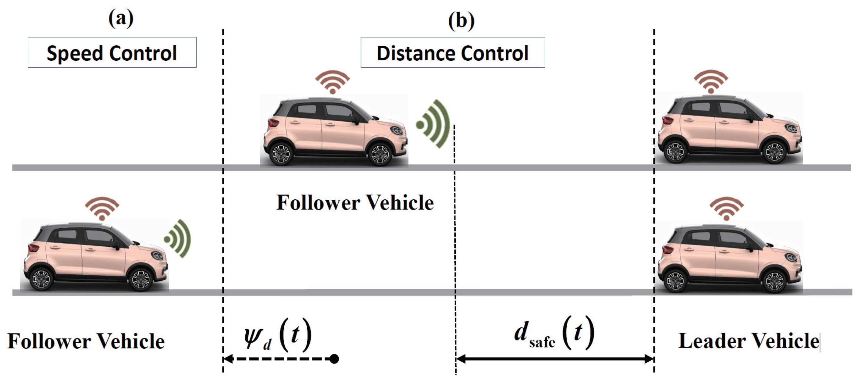
2.2. Adaptive Cruise Control Objective

ACC needs to consider both the safety distance between vehicles and the speed requirements of the vehicles themselves. Therefore, the control objective is to design $F\left(k\right)$ so that the vehicle can operate at a given speed $v_{ref}\left(k\right)$ and keep a safe distance, i.e., $z^L\left(k\right)-z\left(k\right)\ge d_{safe}\left(k\right)$, specifically expressed as [31]

$$\begin{array}{c}\hfill d_{safe}\left(k\right)=d_{st}+hv\left(k\right)\end{array}$$

(2)

where $d_{st}$ is a fixed minimum safety distance; h denotes constant time headway. The structure is shown in Figure 1.

Considering the practical engineering requirements, the controller should have strong robustness and should not rely on accurate $R_i\left(k\right)$, $R_w\left(k\right)$, and $R_r\left(k\right)$ information. Therefore, the goal of ACC is to design time-varying nonlinear control laws based on the speed and distance information for vehicles:

$$\begin{array}{c}\hfill F\left(k\right)=F(k,v\left(k\right),z^L\left(k\right)-z\left(k\right))\end{array}$$

(3)

Substitute Equation (3) into Equation (1) so that

• $z^L\left(k\right)-z\left(k\right)\ge d_{safe}\left(k\right)$;
• On the basis of satisfying the first objective, $v\left(k\right)-v_{ref}\left(k\right)$ should be as small as possible.

3. Main Results

3.1. Model-Free Speed-Prescribed Performance Control Design

When $z^L\left(k\right)-z\left(k\right)$ is very large, only the vehicle speed control needs to be considered, where $v\left(k\right)$ is the output of the system. To design the controller, define the speed error:

$$\begin{array}{c}\hfill {\mathfrak{e}}_v\left(k\right)=v\left(k\right)-v_{ref}\left(k\right)\end{array}$$

(4)

The vehicle’s dynamic model is transformed into

$$\begin{array}{c}\hfill \dot{v}\left(k\right)=\frac{1}{m}F\left(k\right)-f(\eta \left(k\right),v\left(k\right))\end{array}$$

(5)

where

$$\begin{array}{ccc}\hfill & & \eta \left(k\right):=(R_i\left(k\right)-\delta \left(k\right),\rho \left(k\right)),k\ge 0\hfill \\ & & f:={\mathbb{R}}^3\to \mathbb{R},({\eta }_1\left(k\right),{\eta }_2\left(k\right),v\left(k\right))\mapsto \frac{1}{m}\left({\eta }_1\left(k\right)+\frac{1}{2}{\eta }_2\left(k\right)C_{d}Av{\left(k\right)}^2+R_f\left(v\left(k\right)\right)\right)\hfill \end{array}$$

According to the funnel control theory [32], design a vehicle speed-prescribed performance control algorithm:

$$\begin{array}{c}\hfill F_v\left(k\right)=-{\kappa }_v\left(k\right){\mathfrak{e}}_v\left(k\right),{\kappa }_v\left(k\right)=\frac{1}{1-{\varphi }_v{\left(k\right)}^2{\mathfrak{e}}_v{\left(k\right)}^2}\end{array}$$

(6)

where ${\varphi }_v\left(k\right)\in \varphi$ is the prescribed performance function for the speed error. For the initial state, there exists ${\varphi }_v\left(k\right)|v\left(0\right)-v_{ref}\left(0\right)|<1$. This algorithm can ensure that ${\mathfrak{e}}_v\left(k\right)$ is limited within the preset range:

$$\begin{array}{c}\hfill {\mathcal{R}}_{{\varphi }_v}:=\left\{(k,{\mathfrak{e}}_v\left(k\right))\in {\mathbb{R}}_{\ge 0}\times \mathbb{R}|{\varphi }_v\left(k\right)\left|{\mathfrak{e}}_v\left(k\right)\right|<1\right\}\end{array}$$

(7)

3.2. Model-Free Distance-Prescribed Performance Control Design

When $z^L\left(k\right)-z\left(k\right)$ enters the error constraint range of the safe distance $d_{safe}\left(k\right)$, i.e., ${\varphi }_d\left(k\right)\in \Phi ,{\varphi }_d\left(0\right)\ne 0,{\psi }_d(·)={\varphi }_d^{-1}$, it is necessary to consider the distance control of the vehicle, where $z\left(k\right)$ is the output of the system. To design the controller, define the distance-tracking error:

$$\begin{array}{c}\hfill {\mathfrak{e}}_d\left(k\right)=z\left(k\right)-z^L\left(k\right)+d_{safe}\left(k\right)+{\psi }_d\left(k\right)\end{array}$$

(8)

In this case, the vehicle dynamics model described in Equation (1) can be transformed into

$$\begin{array}{c}\hfill \left\{\begin{array}{cc}\dot{z}\left(k\right)\hfill & =v\left(k\right),\hfill \\ \dot{v}\left(k\right)\hfill & =\frac{1}{m}F\left(k\right)-f(\eta \left(k\right),v\left(k\right))\hfill \end{array}\right.\end{array}$$

(9)

According to the PI-funnel control theory [32], design a vehicle distance-prescribed performance control algorithm:

$$\begin{array}{ccc}\hfill F_d\left(k\right)& =& -{\kappa }_d^1\left(k\right){\mathfrak{e}}_d\left(k\right)-{\kappa }_d^2\left(k\right){\mathfrak{e}}_v\left(k\right)\hfill \end{array}$$

(10)

$$\begin{array}{ccc}\hfill {\kappa }_d^1\left(k\right)& =& \frac{{\varphi }_d\left(k\right)}{1-{\varphi }_d\left(k\right)\left|{\mathfrak{e}}_d\left(k\right)\right|}\hfill \end{array}$$

(11)

$$\begin{array}{ccc}\hfill {\kappa }_d^2\left(k\right)& =& \frac{{\varphi }_v\left(k\right)}{1-{\varphi }_v\left(k\right)\left|{\mathfrak{e}}_v\left(k\right)\right|}\hfill \end{array}$$

(12)

where ${\varphi }_d\left(k\right)\in {\varphi }_1$ is the prescribed performance function for the distance error. This algorithm can ensure that ${\mathfrak{e}}_d\left(k\right)$ is limited within the preset range:

$$\begin{array}{c}\hfill {\mathcal{R}}_{{\varphi }_d}:=\left\{(k,{\mathfrak{e}}_d\left(k\right))\in {\mathbb{R}}_{\ge 0}\times \mathbb{R}|{\varphi }_d\left(k\right)\left|{\mathfrak{e}}_d\left(k\right)\right|<1\right\}\end{array}$$

(13)

Remark 1.

Because of the strict requirement of distance control to ensure $z\left(k\right)-z^L\left(k\right)\ge d_{safe}\left(k\right)$, the definition of distance error ${\mathfrak{e}}_d\left(k\right)$ has an additional term of ${\psi }_d\left(k\right)$ compared to the definition of speed error ${\mathfrak{e}}_v\left(k\right)$, and the control objective is $d_{safe}\left(k\right)<z\left(k\right)-z^L\left(k\right)<d_{safe}\left(k\right)+2{\psi }_d\left(k\right)$.

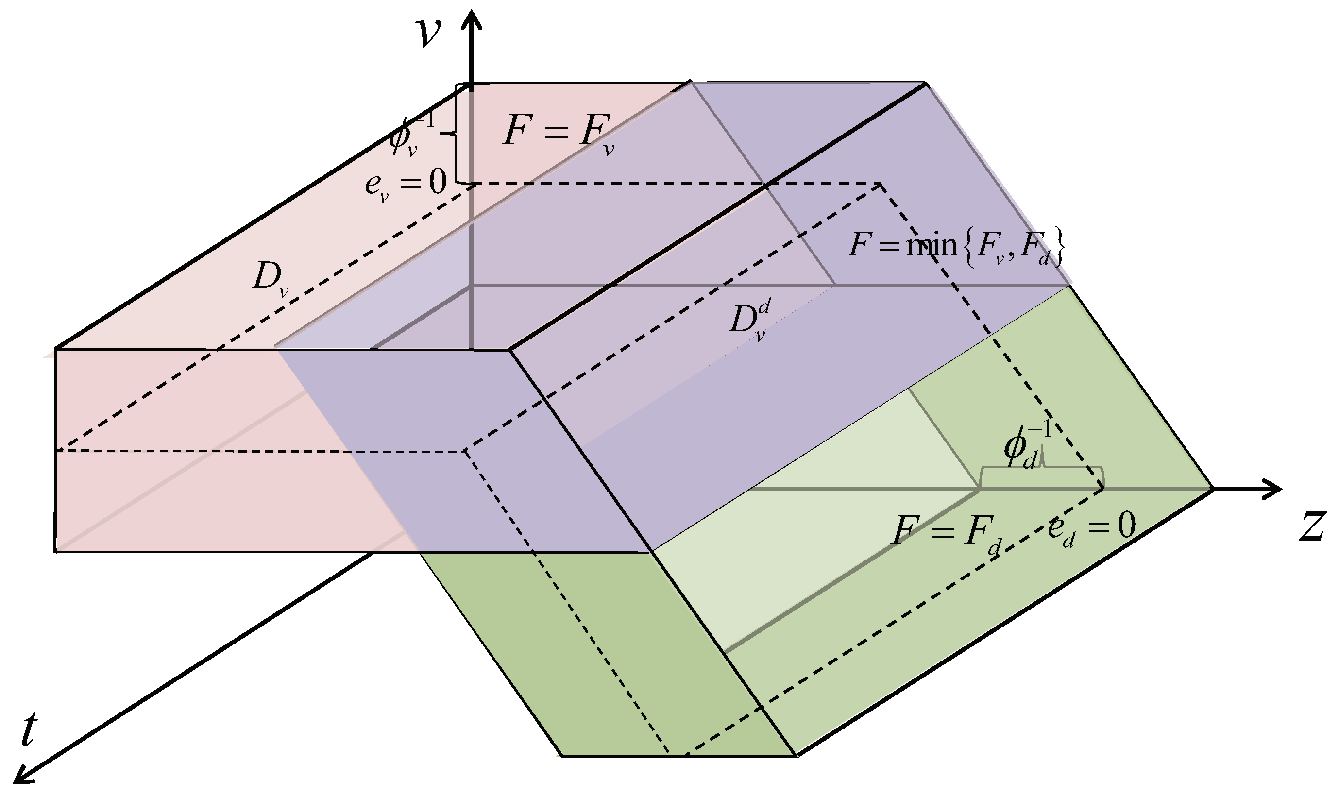
3.3. Integrated Algorithm Design for Vehicle Speed and Distance Control

The vehicle speed-prescribed performance control takes speed as the system output, without considering objective 1. When the vehicle approaches the front vehicle, it needs to meet objective 2. Therefore, the entire process of vehicle adaptive cruise control needs to meet the following additional conditions:

• When the vehicle enters the safe-distance error constraint range, i.e., $z\left(k\right)-z^L\left(k\right)+d_{safe}\left(k\right)+{\psi }_d\left(k\right)<{\psi }_d\left(k\right)$, the speed-prescribed performance control should automatically switch to distance-prescribed performance control;
• When distance-prescribed performance control is in effect, try to ensure $v\left(k\right)<v_{ref}\left(k\right)+{\psi }_v{\left(k\right)}^{-1}$. If $v\left(k\right)>v_{ref}\left(k\right)+{\psi }_v{\left(k\right)}^{-1}$ (leader deceleration), it should not switch back to the speed-prescribed performance control.

The problem of the integrated control algorithm for vehicle speed and distance can be summarized as follows: when $z\left(k\right)=z^L\left(k\right)-d_{\mathrm{safe}}\left(k\right)$, ${\kappa }_d^1\left(k\right)\nearrow \infty$, ${\kappa }_d^2\left(k\right)\nearrow \infty$; when $v\left(k\right)=v_{\mathrm{ref}}\left(k\right)-{\varphi }_v{\left(k\right)}^{-1}$, ${\kappa }_v\left(k\right)\nearrow \infty$. For this purpose, in the intersection area of speed- and distance-prescribed performance, i.e., $\left(k,{\mathfrak{e}}_v\left(k\right)\right)\in {\mathcal{R}}_{{\varphi }_v}\wedge \left(k,{\mathfrak{e}}_d\left(k\right)\right)\in {\mathcal{R}}_{{\varphi }_d}$, the control input is set as $min\left\{-{\kappa }_v\left(k\right){\mathfrak{e}}_v\left(k\right),-{\kappa }_d^1\left(t\right){\mathfrak{e}}_d\left(k\right)-{\kappa }_d^2\left(t\right){\mathfrak{e}}_k\left(k\right)\right\}$, see Figure 2.

Therefore, the integrated control for vehicle speed and distance control can be expressed as

$$\begin{array}{ccc}\hfill F\left(k\right)& =& \left\{\begin{array}{c}\hfill -{\kappa }_v\left(k\right){\mathfrak{e}}_v\left(k\right),{\mathfrak{e}}_d\left(k\right)\le -{\varphi }_d{\left(k\right)}^{-1}\wedge \left(k,{\mathfrak{e}}_v\left(k\right)\right)\in {\mathcal{R}}_{{\varphi }_v}\\ \hfill -{\kappa }_d^1\left(k\right){\mathfrak{e}}_d\left(k\right)-{\kappa }_d^2\left(k\right){\mathfrak{e}}_v\left(k\right),{\mathfrak{e}}_v\left(k\right)\le -{\varphi }_v{\left(k\right)}^{-1}\wedge \left(k,{\mathfrak{e}}_d\left(k\right)\right)\in {\mathcal{R}}_{{\varphi }_d}\\ \hfill min\left\{F_d\left(k\right),F_v\left(k\right)\right\},\left(k,{\mathfrak{e}}_v\left(k\right)\right)\in {\mathcal{R}}_{{\varphi }_v}\wedge \left(k,{\mathfrak{e}}_d\left(k\right)\right)\in {\mathcal{R}}_{{\varphi }_d}\end{array}\right.\hfill \\ \hfill {\kappa }_v\left(k\right)& =& \frac{1}{1-{\varphi }_v{\left(k\right)}^2{\mathfrak{e}}_v{\left(k\right)}^2}\hfill \\ \hfill {\mathfrak{e}}_v\left(k\right)& =& v\left(k\right)-v_{\mathrm{ref}}\left(k\right)\hfill \\ \hfill {\kappa }_d^1\left(k\right)& =& \frac{{\varphi }_d^{}\left(k\right)}{1-{\varphi }_d^{}\left(k\right)\left|{\mathfrak{e}}_d\left(k\right)\right|},{\kappa }_d^2\left(k\right)=\frac{{\varphi }_v^{}\left(k\right)}{1-{\varphi }_v^{}\left(k\right)\left|{\mathfrak{e}}_v\left(k\right)\right|}\hfill \\ \hfill {\mathfrak{e}}_d\left(k\right)& =& z\left(k\right)-z^L\left(k\right)+d_{\mathrm{safe}}\left(k\right)+{\psi }_d\left(k\right)\hfill \end{array}$$

(14)

3.4. Algorithm Feasibility and Stability Analysis

In the designed prescribed performance adaptive cruise control, the solution $(z,v)$ of Equation (1) is limited by the open set $\mathcal{D}$. For a fixed $k>0$, the set $\left\{(z,v)\right|(k,z,v)\in \mathcal{D}\}\subseteq {\mathbb{R}}^2$ is nonconvex, as shown in Figure 2. Therefore, the following proof method is provided, and the specific conclusion is shown in Theorem 1.

Theorem 1.

For the vehicle dynamics system described in Equation (1), if the desired running speed of the vehicle $v_{ref}\left(k\right)$ and the leader vehicle’s positions $z^L$ and ${\dot{z}}^L$ are bounded, substituting the controller (14) into the vehicle dynamics system (1) can obtain a solved closed-loop system. Each solution of the closed-loop system can be generalized to a maximum solution $\left(z,v\right):\left[0,w\right)\to {\mathbb{R}}^2,w\in \left(0,\infty \right]$, and the solution has the following properties:

• The speed $v\left(k\right)$ and control input $F\left(k\right)$ are bounded;
• There exists $\epsilon >0$, for all $k>0$, if the following conditions are satisfied.

  $${\mathfrak{e}}_v\left(k\right)\le {\varphi }_v{\left(k\right)}^{-1}-\epsilon ,{\mathfrak{e}}_d\left(k\right)\le {\varphi }_d{\left(k\right)}^{-1}-\epsilon ,$$

  $$\epsilon \le \left\{max\left\{0,{\varphi }_v{\left(k\right)}^{-1}+{\mathfrak{e}}_v\left(k\right)\right\}+max\left\{0,{\varphi }_d{\left(k\right)}^{-1}+{\mathfrak{e}}_d\left(k\right)\right\}\right\}$$

Proof. 

Step 1: Explanation of the existence of the maximum solution. Definition:

$$\begin{array}{c}{\psi }_v\left(t\right):={\varphi }_v{\left(k\right)}^{-1},{\psi }_d\left(k\right):={\varphi }_d{\left(t\right)}^{-1}\hfill \\ f:{\mathbb{R}}_{\ge 0}\times \mathbb{R}\to \mathbb{R},\left(k,v\right)\mapsto -\frac{1}{m}\left(R_{\mathrm{i}}\left(k\right)+R_{\mathrm{w}}\left(k,v\right)+R_{\mathrm{f}}\left(v\right)-\delta \left(k\right)\right)\hfill \\ F:\mathcal{D}\to {\mathbb{R}}^2,\left(k,z,v\right)\mapsto \hfill \\ \left\{\begin{array}{c}\left(\begin{array}{c}v\\ -\frac{1}{m}\frac{v-v_{\mathrm{ref}}\left(k\right)}{1-{\varphi }_v{\left(k\right)}^2{\left|v-v_{\mathrm{ref}}\left(k\right)\right|}^2}+f\left(k,v\right)\end{array}\right),\mathrm{if}\left(k,z,v\right)\in {\mathcal{D}}_v\\ \left(\begin{array}{c}v\\ -\frac{1}{m}\frac{v-v_{\mathrm{ref}}\left(k\right)}{1-{\varphi }_v{\left(k\right)}^2{\left|v-v_{\mathrm{ref}}\left(k\right)\right|}^2}-\frac{1}{m}\frac{z\left(k\right)-z^L\left(k\right)+d_{\mathrm{st}}+hv\left(k\right)+{\psi }_d\left(t\right)}{1-{\varphi }_d{\left(k\right)}^2{\left|z\left(k\right)-z^L\left(k\right)+d_{\mathrm{st}}+hv\left(k\right)+{\psi }_d\left(k\right)\right|}^2}+f\left(k,v\right)\end{array}\right),\mathrm{if}\left(k,z,v\right)\in {\mathcal{D}}_d\\ \left(\begin{array}{c}v\\ \frac{1}{m}min\left\{\begin{array}{c}-\frac{v-v_{\mathrm{ref}}\left(k\right)}{1-{\varphi }_v{\left(k\right)}^2{\left|v-v_{\mathrm{ref}}\left(k\right)\right|}^2},\\ -\frac{1}{m}\frac{v-v_{\mathrm{ref}}\left(k\right)}{1-{\varphi }_v{\left(k\right)}^2{\left|v-v_{\mathrm{ref}}\left(k\right)\right|}^2}-\frac{1}{m}\frac{z\left(k\right)-z^L\left(k\right)+d_{\mathrm{st}}+hv\left(k\right)+{\psi }_d\left(k\right)}{1-{\varphi }_d{\left(k\right)}^2{\left|z\left(t\right)-z^L\left(t\right)+d_{\mathrm{st}}+hv\left(k\right)+{\psi }_d\left(k\right)\right|}^2}\end{array}\right\}+f\left(k,v\right)\end{array}\right),\\ \mathrm{if}\left(k,z,v\right)\in {\mathcal{D}}_v^d\hfill \end{array}\right.\hfill \end{array}$$

(15)

Then, the closed-loop initial value problem formed by Formulas (1) and (2) is equivalent to

$$\begin{array}{c}\hfill \left(\begin{array}{c}\dot{z}\left(k\right)\hfill \\ \dot{v}\left(k\right)\hfill \end{array}\right)=F\left(z\left(k\right),v\left(k\right),k\right),\left(z\left(0\right),v\left(0\right)=z^0,v^0\right)\end{array}$$

(16)

Due to $R_i\left(k\right),R_f\left(v\right),R_w(k,v)$ being continuous, $\delta \left(k\right)$ is bounded, and f is measurable, locally integrable, and continuous for v. In addition, ${\varphi }_d\left(k\right),{\varphi }_v\left(k\right),v_{ref}\left(k\right),z^L\left(k\right)$ are continuous, and we can conclude that F is measurable, locally integrable, and continuous for v; $\mathcal{D}$ satisfies $\left(0,z^0,v^0\right)\in \mathcal{D}$. Therefore, there exists a weakly differentiable solution that can be generalized to an extreme solution $\left(z,v\right):\left[0,w\right)\to {}^2,w\in \left(0,\infty \right]$. Furthermore, the closed interval of $(z,v)$ is not a compact set of $\mathcal{D}$. For the subsequent analysis, the set $[0,w)$ is divided into two parts:

$$\begin{array}{ccc}& & N_v:=\left\{k\in \left[0,w\right)\left|\begin{array}{c}\left(k,z\left(k\right),v\left(k\right)\right)\in {\mathcal{D}}_v\vee \hfill \\ (\left(k,z\left(k\right),v\left(k\right)\right)\in {\mathcal{D}}_v^d\wedge \hfill \\ min\left\{-{\kappa }_v\left(k\right){\mathfrak{e}}_v\left(k\right),-{\kappa }_d^1\left(t\right){\mathfrak{e}}_d\left(k\right)-{\kappa }_d^2\left(k\right){\mathfrak{e}}_v\left(k\right)\right\}=-{\kappa }_v\left(k\right){\mathfrak{e}}_v\left(k\right))\hfill \end{array}\right.\right\}\hfill \\ & & N_d:=\left\{k\in \left[0,w\right)\left|\begin{array}{c}\left(k,z\left(k\right),v\left(k\right)\right)\in {\mathcal{D}}_d\vee \hfill \\ \left(\begin{array}{c}min\left\{-{\kappa }_v\left(t\right){\mathfrak{e}}_v\left(k\right),-{\kappa }_d^1\left(k\right){\mathfrak{e}}_d\left(k\right)-{\kappa }_d^2\left(k\right){\mathfrak{e}}_v\left(k\right)\right\}=\hfill \\ -{\kappa }_d^1\left(k\right){\mathfrak{e}}_d\left(k\right)-{\kappa }_d^2\left(k\right){\mathfrak{e}}_v\left(k\right)\wedge \left(k,z\left(k\right),v\left(k\right)\right)\in {\mathcal{D}}_v^d\hfill \end{array}\right)\hfill \end{array}\right.\right\}\hfill \end{array}$$

(17)

Step 2: Illustration of the boundedness of the speed v and vehicle distance $z-z^L$.

• $v\left(k\right)$ is bounded on $N_v$. Assuming that the velocity is $v\left(k\right)$ unbounded on $N_v$, due to $v_{ref}\left(k\right)$ being bounded and ${\psi }_v{|}_{\left[\epsilon ,\infty \right)}$ being continuous and bounded, there exists $k^{*}\in N_v,k^{*}>0$ such that $\left|v\left(k^{*}\right)\right|>v_{\mathrm{ref}}\left(k^{*}\right)+{\psi }_v\left(k^{*}\right)$. This contradicts $\left(k^{*},z\left(k^{*}\right),v\left(k^{*}\right)\right)\in \mathcal{D}$. By using the same method, it can be proven that the speed $v\left(k\right)$ is bounded on $N_d$.
• $z^L-z$ is bounded. Due to $\left(k,z\left(k\right),v\left(k\right)\right)\in \mathcal{D},k\in \left[0,w\right)$ and ${\mathfrak{e}}_d\left(k\right)<{\psi }_d\left(k\right)$, we can conclude that $x\left(k\right)=hv\left(k\right)+z\left(k\right)-z^L\left(k\right)<d_{\mathrm{st}},k\in \left[0,w\right)$. Define $\mathfrak{z}=z^L-z,\mu =\frac{1}{h}$, and we have $\dot{\mathfrak{z}}\left(k\right)=-\mu k\left(k\right)-\mu x\left(k\right)+{\dot{z}}^L\left(k\right),\mathfrak{z}\left(0\right)=z^L\left(0\right)-z^0$. Furthermore, $\mathfrak{z}\left(k\right)={\mathfrak{e}}^{-\mu k}\mathfrak{z}\left(0\right)+{\int }_0^k{\mathfrak{e}}^{-\mu \left(k-s\right)}\left({\dot{z}}^L\left(k\right)-\mu x\left(s\right)\right)\mathrm{ds}\ge -\left|\mathfrak{z}\left(0\right)\right|-{\int }_0^k{\mathfrak{e}}^{-\mu \left(k-s\right)}\left({∥{\dot{z}}^L∥}_{\infty }+\mu d_{\mathrm{st}}\right)\ge -\infty$.

Step 3: Illustration of the boundedness of $F\left(k\right)$.

For $k_0,k\in (0,w)$, $t\ge t_0$, and $(k,z,v)\in {\mathcal{D}}_v$, there exists $F\left(k\right)=-{\kappa }_v\left(k\right){\mathfrak{e}}_v\left(k\right)$ and ${\mathfrak{e}}_v\left(k\right)\le {\psi }_v\left(k\right)-\epsilon$; therefore, we have

$$\begin{array}{ccc}\hfill \left|F\left(k\right)\right|& =& \frac{\left|{\mathfrak{e}}_v\left(k\right)\right|}{\left(1-{\varphi }_v\left(k\right)\left|{\mathfrak{e}}_v\left(k\right)\right|\right)\left(1+{\varphi }_v\left(k\right)\left|{\mathfrak{e}}_v\left(k\right)\right|\right)}\hfill \\ & \le & \frac{\left|{\mathfrak{e}}_v\left(k\right)\right|}{\left(1-{\varphi }_v\left(k\right)\left|{\mathfrak{e}}_v\left(k\right)\right|\right)}\le \frac{\left|{\mathfrak{e}}_v\left(k\right)\right|}{{\varphi }_v\left(k\right)\epsilon }\le \frac{1}{\epsilon }\underset{s\ge k_0}{sup}{\psi }_v{\left(s\right)}^2\hfill \end{array}$$

(18)

Similarly, for $k_0,k\in (0,w)$, $t\ge t_0$ and $(k,z,v)\in {\mathcal{D}}_d$, we can prove

$$\begin{array}{c}\hfill \left|F\left(k\right)\right|\le \frac{1}{\epsilon }\underset{s\ge k_0}{sup}{\psi }_d{\left(s\right)}^2\end{array}$$

(19)

For $k_0,k\in (0,w)$, $t\ge t_0$, and $(k,z,v)\in {\mathcal{D}}_v^d$, we prove that

$$\begin{array}{c}\hfill \left|F\left(k\right)\right|\le C_{k_0}:=\frac{2}{\epsilon }\underset{s\ge k_0}{sup}{\psi }_d{\left(s\right)}^2+\frac{1}{\epsilon }\underset{s\ge k_0}{sup}{\psi }_v{\left(s\right)}^2\end{array}$$

(20)

• If ${\mathfrak{e}}_v\left(k\right)>0$ and ${\mathfrak{e}}_d\left(k\right)<0$, there is $F\left(k\right)=-{\kappa }_v\left(k\right){\mathfrak{e}}_v\left(k\right)$; then, $rF\left(k\right)\le C_{k_0}$.
• If ${\mathfrak{e}}_v\left(k\right)<0$ and ${\mathfrak{e}}_d\left(k\right)>0$, there is $F\left(k\right)=-{\kappa }_d^1\left(k\right){\mathfrak{e}}_d\left(k\right)-{\kappa }_d^2\left(k\right){\mathfrak{e}}_v\left(k\right)$; then, $F\left(k\right)\le C_{k_0}$.
• If ${\mathfrak{e}}_v\left(k\right)>0$ and ${\mathfrak{e}}_d\left(k\right)>0$, there exists ${\psi }_v\left(k\right)-{\mathfrak{e}}_v\left(k\right)\ge \epsilon$ and ${\psi }_d\left(k\right)-{\mathfrak{e}}_d\left(k\right)\ge \epsilon$ such that ${\kappa }_v\left(k\right)\le \frac{1}{\epsilon {\varphi }_v\left(k\right)}$ and ${\kappa }_d^1\left(k\right)\le \frac{1}{\epsilon {\varphi }_d\left(k\right)}$; then, $-{\kappa }_d^1\left(k\right){\mathfrak{e}}_d\left(k\right)-{\kappa }_d^2\left(k\right){\mathfrak{e}}_v\left(k\right)\ge -\frac{1}{{\epsilon {\varphi }_d\left(k\right)}^2}-\frac{1}{{\epsilon {\varphi }_v\left(k\right)}^2}$, $-{\kappa }_v\left(k\right){\mathfrak{e}}_v\left(k\right)\ge -\frac{1}{{\epsilon {\varphi }_v\left(k\right)}^2}$. Furthermore,

  $$\begin{array}{c}\hfill 0\ge F\left(k\right)=min\left\{-{\kappa }_v\left(k\right){\mathfrak{e}}_v\left(k\right),-{\kappa }_d^1\left(k\right){\mathfrak{e}}_d\left(k\right)-{\kappa }_d^2\left(k\right){\mathfrak{e}}_v\left(k\right)\right\}\ge -\frac{1}{\epsilon {\varphi }_d{\left(k\right)}^2}-\frac{1}{\epsilon {\varphi }_v{\left(k\right)}^2}\ge C_{k_0}\end{array}$$
  Therefore, we have $F\left(k\right)\le C_{k_0}$.
• If ${\mathfrak{e}}_v\left(k\right)<0$ and ${\mathfrak{e}}_d\left(k\right)<0$, there exists $\epsilon \le max\left\{0,{\psi }_v\left(k\right)+{\mathfrak{e}}_v\left(k\right)\right\}+max\left\{0,{\psi }_d\left(k\right)+{\mathfrak{e}}_d\left(k\right)\right\}$. When $(k,z,v)\in {\mathcal{D}}_v^d$, we have $max\left\{{\psi }_v\left(k\right)+{\mathfrak{e}}_v\left(k\right),{\psi }_d\left(k\right)+{\mathfrak{e}}_d\left(k\right)\right\}\ge \frac{\epsilon }{2}$. Thus, we have ${\psi }_v\left(k\right)+{\mathfrak{e}}_v\left(k\right)\ge \frac{\epsilon }{2}$ or ${\psi }_d\left(k\right)+{\mathfrak{e}}_d\left(k\right)\ge \frac{\epsilon }{2}$.

If ${\psi }_v\left(k\right)+{\mathfrak{e}}_v\left(k\right)\ge \frac{\epsilon }{2}$, we have

$$\begin{array}{c}\hfill {\kappa }_v\left(k\right)=\frac{1}{\left(1-{\varphi }_v\left(k\right){\mathfrak{e}}_v\left(k\right)\right)\left(1+{\varphi }_v\left(k\right){\mathfrak{e}}_v\left(k\right)\right)}\le \frac{1}{\left(1+{\varphi }_v\left(k\right){\mathfrak{e}}_v\left(k\right)\right)}\le \frac{2}{{\varphi }_v\left(k\right)\epsilon }\end{array}$$

(21)

Similarly, if ${\psi }_d\left(k\right)+{\mathfrak{e}}_d\left(k\right)\ge \frac{\epsilon }{2}$, we have

$$\begin{array}{c}\hfill {\kappa }_d\left(k\right)\le \frac{2}{{\varphi }_d\left(k\right)\epsilon }\end{array}$$

(22)

Furthermore, we have $-{\kappa }_v\left(k\right){\mathfrak{e}}_v\left(k\right)\le \frac{2}{\epsilon {\varphi }_v{\left(k\right)}^2}$ or $-{\kappa }_d\left(k\right){\mathfrak{e}}_d\left(k\right)\le \frac{2}{\epsilon {\varphi }_d{\left(k\right)}^2}$.

Therefore, we have

$$\begin{array}{c}\hfill 0\le F\left(k\right)=min\left\{-{\kappa }_v\left(k\right){\mathfrak{e}}_v\left(k\right),-{\kappa }_d^1\left(k\right){\mathfrak{e}}_d\left(k\right)-{\kappa }_d^2\left(k\right){\mathfrak{e}}_v\left(k\right)\right\}\le \frac{2}{\epsilon {\varphi }_d{\left(k\right)}^2}+\frac{2}{\epsilon {\varphi }_v{\left(k\right)}^2}\ge C_{k_0}\end{array}$$

□

4. Simulations and Discussion

The effectiveness of the designed algorithm is demonstrated in three daily traffic scenarios. The main contribution of this paper is that the designed controller only requires the speed and position information of the vehicle, without the need for accurate models or parameters. The vehicle parameters are listed in

Table 1. Parameters of vehicle.

Parameter	Value	Parameter	Value	Parameter	Value
m/kg	1300	$\rho$/(kg/m3)	1.3	Cr	0.01
A/m2	2.4	$\theta \left(k\right)$	2	Cd	0.32

and are only used for model updates. The vehicle interference is $\delta (·)=0$; the vehicle spacing strategy parameters are $h=0.5$ s and $d_{st}=2$ m; the initial state of the vehicle is $z^0=0$ m and $v^0=15$ m/s; the initial state of the leader vehicle is $z^L\left(0\right)=20$ m and $v^L\left(0\right)=30$ m/s; the reference speed for the following vehicle is $v_{ref}=36$ m/s; the velocity error constraint function is ${\varphi }_v\left(k\right)={\left(22{\mathfrak{e}}^{-0.2k}+0.2\right)}^{-1}$; and the spacing error constraint function is ${\varphi }_d\left(k\right)=10$.

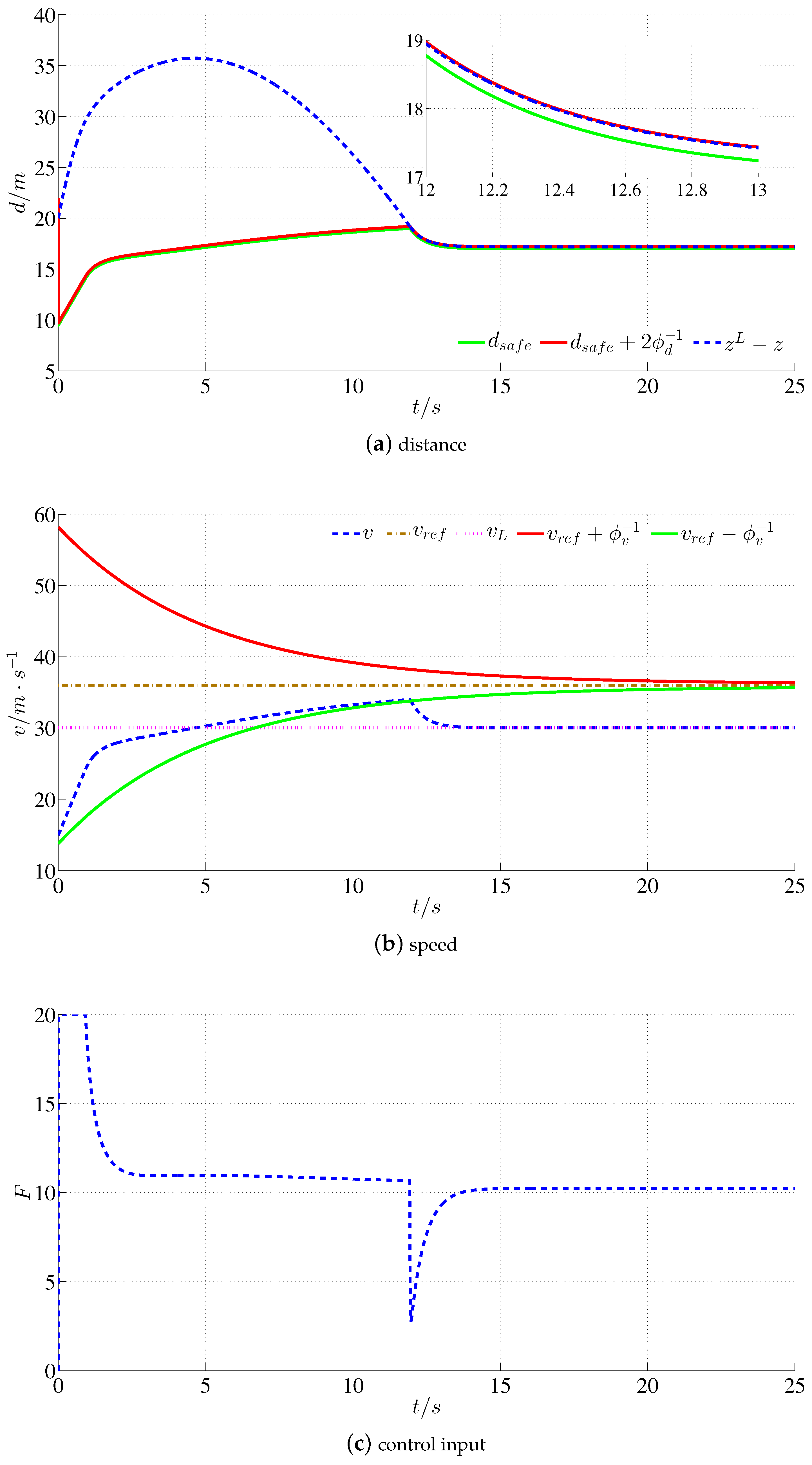
4.1. Scenario 1: Approaching the Leader Car and Following the Leader

In this scenario, it is assumed that the follower vehicle is far from the pilot vehicle, i.e., $z^L\left(0\right)>>z\left(0\right)$, and their speeds satisfy $v^L\left(0\right)>v\left(0\right)$, but the follower vehicle’s speed is less than the reference speed set by itself, i.e., $v\left(0\right)<v_{ref}$.

Figure 3 shows the results of scenario 1. In the 0–5 s stage, the distance between the two vehicles gradually increases due to $v^L\left(k\right)>z\left(k\right)$, and it should be pointed out that the speed of the vehicle remains within the preset range. During the 5–11.5 s stage, the distance between the two vehicles gradually decreases due to $v^L\left(k\right)<z\left(k\right)$. After 11.5 s, the follower vehicle enters the safe distance range, and the controller switches from speed-prescribed performance control to distance-prescribed performance control. The two vehicles operate within the preset safe distance range while their speeds gradually converge.

Remark 2.

It should be emphasized that thanks to the novel stability analysis method proposed in this article, the designed ACC makes switching between the speed and distance control of the vehicle very smooth.

Remark 3.

In the speed control stage, the controller can constrain the speed error within a preset range, thereby ensuring the smoothness of the vehicle operation. In the distance control stage, the controller can constrain the distance error within a predetermined range, thereby achieving collision avoidance.

4.2. Scenario 2: Rapid Deceleration of Leader Vehicle

In this scenario, the leader car suddenly brakes sharply and decelerates from 30 m/s to 1 m/s with 5 m/s² deceleration at 15 s.

Figure 4 shows the results of scenario 2. When the leader vehicle decelerates sharply, the distance-prescribed performance control algorithm can control the vehicle to brake with the leader vehicle within the preset safe spacing range to avoid collision and achieve emergency avoidance.

Remark 4.

Due to the controller constraining the range of the distance error variation, when the leader vehicle decelerates urgently, the following vehicle will also decelerate urgently without overshoot.

4.3. Scenario 3: Frequent Start and Stop of Leader Vehicle

Figure 5 shows the results of scenario 3. During the 1–25 s stage, the follower vehicles are all within the distance-prescribed performance control range, and the distance between the follower and the leader is always within the preset safety range. When the leader car stops or starts at 7.5 s, 10.5 s, 17 s, and 23.5 s, the follower car and the leader car keep synchronized to start and stop.

4.4. Comparative Experiment

To better illustrate the difference between the existing algorithm, PI-based ACC is simulated based on scenario 1. Actually, PI-based ACC can be seen as a special case of (10), where ${\kappa }_d^1\left(k\right)$ and ${\kappa }_d^2\left(k\right)$ are constants. In this experiment, ${\kappa }_d^1\left(k\right)=500$ and ${\kappa }_d^1\left(k\right)=20$. The simulation results are shown in Figure 6. From Figure 6a, the PI-based ACC vehicle can track the leader vehicle with the desired speed and distance, but the tracking error cannot be limited in the prescribed range. In addition, PI-based ACC takes speed tracking and distance tracking as the overall target and cannot control each single target separately at different stages. Compared to PI-based ACC, the proposed algorithm has a strong decoupling ability and can achieve the velocity- or distance-tracking control at different stages. Therefore, the proposed algorithm in this paper is more flexible.

5. Conclusions

This paper proposes a model-free ACC speed- and distance-switching prescribed performance control algorithm. The algorithm consists of two parts: speed-prescribed performance control and collision avoidance distance-prescribed performance control. If the follower is far from the leader vehicle, a speed-prescribed performance controller is used to adjust the follower vehicle’s speed to the desired predefined speed according to the prescribed range. If the follower vehicle approaches the leader vehicle, the collision avoidance distance-prescribed performance control adjusts the distance between the follower and leader vehicle to keep a safe distance between the two vehicles.

(1) Regarding the information required for the control algorithm, the existing ACC algorithm must establish an accurate system model, while strictly ensuring safety, and obtain the position, speed, or acceleration information of the leader vehicle. The proposed model-free adaptive cruise control algorithm only requires speed information of the controlled vehicle and distance information from the vehicle in front.

(2) Regarding the control effect of the control algorithm, the developed algorithm ensures that the vehicle’s operating speed and distance strictly change smoothly within the prescribed spatial range, and there is no overshoot phenomenon during the initial state adjustment, emergency braking, and frequent start and stop stages. It can meet the various control requirements of ACC for speed, spacing, and collision avoidance.

Similar to numerous current methods in robust control, the controller we have developed is not immediately compatible with hardware platforms and requires integration with additional power electronics techniques. Going forward, a complete ACC physical framework will be set up under the control paradigm proposed in this study.

References

1. Zhang, L.; Wu, G.; Guo, X. Vehicular multi-objective adaptive cruise control algorithm. J. Xi’An Jiaotong Univ. 2016, 50, 136–143. [Google Scholar]
2. Zhang, Y.; Song, J. Model-free robust backstepping adaptive cruise control. Int. J. Aerosp. Eng. 2023, 2023, 8839650. [Google Scholar] [CrossRef]
3. Pin, Q.P.; Kang, P.S.; Lei, H.X.; Min, W.F.; Qian, W. Influence of different vehicle operating conditions on driving safety of CACC platoon. J. Transp. Syst. Eng. Inf. Technol. 2019, 19, 33–42. [Google Scholar]
4. Hua, X.; Yang, J.W.W. Redesign and experimental evaluation of cooperative adaptive cruise control system. J. Transp. Syst. Eng. Inf. Technol. 2019, 19, 52–60. [Google Scholar]
5. Karafyllis, I.; Theodosis, D.; Papageorgiou, M. Lyapunov-based two-dimensional cruise control of autonomous vehicles on lane-free roads. Automatica 2022, 145, 110517. [Google Scholar] [CrossRef]
6. Theodosis, D.; Karafyllis, I.; Papageorgiou, M. Cruise controllers for lane-free ring-roads based on control Lyapunov functions. J. Frankl. Inst. 2023, 360, 6131–6161. [Google Scholar] [CrossRef]
7. Ahmad, E.; Iqbal, J.; Arshad Khan, M.; Liang, W.; Youn, I. Predictive control using active aerodynamic surfaces to improve ride quality of a vehicle. Electronics 2020, 9, 1463. [Google Scholar] [CrossRef]
8. Hailemichael, H.; Ayalew, B.; Kerbel, L.; Ivanco, A.; Loiselle, K. Safety filtering for reinforcement learning-based adaptive cruise control. IFAC-PapersOnLine 2022, 55, 149–154. [Google Scholar] [CrossRef]
9. Shakouri, P.; Ordys, A. Nonlinear model predictive control approach in design of adaptive cruise control with automated switching to cruise control. Control Eng. Pract. 2014, 26, 160–177. [Google Scholar] [CrossRef]
10. Zhang, H.; Liang, J.; Zhang, Z. Active fault tolerant control of adaptive cruise control system considering vehicle-borne millimeter wave radar sensor failure. IEEE Access 2020, 8, 11228–11240. [Google Scholar] [CrossRef]
11. Song, J.; Yan, M.; Ju, Y.; Yang, P. Nonlinear gain feedback adaptive DSC for a class of uncertain nonlinear systems with asymptotic output tracking. Nonlinear Dyn. 2019, 98, 2195–2210. [Google Scholar] [CrossRef]
12. Lin, Y.-C.; Nguyen, H.-L.T.; Wang, C.-H. Adaptive neuro-fuzzy predictive control for design of adaptive cruise control system. In Proceedings of the 2017 IEEE 14th International Conference on Networking, Sensing and Control (ICNSC), Calabria, Italy, 16–18 May 2017; pp. 767–772. [Google Scholar]
13. Flores, C.; Milanés, V. Fractional-order-based ACC/CACC algorithm for improving string stability. Transp. Res. Part C Emerg. Technol. 2018, 95, 381–393. [Google Scholar] [CrossRef]
14. Li, X.; Zeng, C.; Luo, J.; Hu, J.; Wang, X. Research on adaptive cruise control algorithm based on linear quadratic optimal control. J. Wuhan Univ. Technol. Inf. Manag. Eng. 2019, 41, 81–86. [Google Scholar]
15. Wang, P.; Deng, H.; Zhang, J.; Wang, L.; Zhang, M.; Li, Y. Model predictive control for connected vehicle platoon under switching communication topology. IEEE Trans. Intell. Transp. Syst. 2021, 23, 7817–7830. [Google Scholar] [CrossRef]
16. Ganji, B.; Kouzani, A.Z.; Khoo, S.Y.; Shams-Zahraei, M. Adaptive cruise control of a HEV using sliding mode control. Expert Syst. Appl. 2014, 41, 607–615. [Google Scholar] [CrossRef]
17. Milanés, V.; Villagrá, J.; Godoy, J.; González, C. Comparing fuzzy and intelligent PI controllers in stop-and-go manoeuvres. IEEE Trans. Control Syst. Technol. 2011, 20, 770–778. [Google Scholar] [CrossRef]
18. Lidström, K.; Sjöberg, K.; Holmberg, U.; Andersson, J.; Bergh, F.; Bjäde, M.; Mak, S. A modular CACC system integration and design. IEEE Trans. Intell. Transp. Syst. 2012, 13, 1050–1061. [Google Scholar] [CrossRef]
19. Weißmann, A.; Görges, D.; Lin, X. Energy-optimal adaptive cruise control combining model predictive control and dynamic programming. Control Eng. Pract. 2018, 72, 125–137. [Google Scholar] [CrossRef]
20. Li, S.E.; Jia, Z.; Li, K.; Cheng, B. Fast online computation of a model predictive controller and its application to fuel economy-oriented adaptive cruise control. IEEE Trans. Intell. Transp. Syst. 2014, 16, 1199–1209. [Google Scholar] [CrossRef]
21. Bageshwar, V.L.; Garrard, W.L.; Rajamani, R. Model predictive control of transitional maneuvers for adaptive cruise control vehicles. IEEE Trans. Veh. Technol. 2004, 53, 1573–1585. [Google Scholar] [CrossRef]
22. Li, S.; Li, K.; Rajamani, R.; Wang, J. Model predictive multi-objective vehicular adaptive cruise control. IEEE Trans. Control Syst. Technol. 2010, 19, 556–566. [Google Scholar] [CrossRef]
23. Magdici, S.; Althoff, M. Adaptive cruise control with safety guarantees for autonomous vehicles. IFAC-PapersOnLine 2017, 50, 5774–5781. [Google Scholar] [CrossRef]
24. Song, J.-c.; Ju, Y.-f. Distributed adaptive sliding mode control for vehicle platoon with uncertain driving resistance and actuator saturation. Complexity 2020, 2020, 7581517. [Google Scholar] [CrossRef]
25. Berger, T.; Lê, H.H.; Reis, T. Funnel control for nonlinear systems with known strict relative degree. Automatica 2018, 87, 345–357. [Google Scholar] [CrossRef]
26. Cheng, S.; Li, L.; Mei, M.-m.; Nie, Y.-l.; Zhao, L. Multiple-objective adaptive cruise control system integrated with DYC. IEEE Trans. Veh. Technol. 2019, 68, 4550–4559. [Google Scholar] [CrossRef]
27. Yoon, S.; Jeon, H.; Kum, D. Predictive cruise control using radial basis function network-based vehicle motion prediction and chance constrained model predictive control. IEEE Trans. Intell. Transp. Syst. 2019, 20, 3832–3843. [Google Scholar] [CrossRef]
28. Berger, T.; Rauert, A.L. Funnel cruise control. Automatica 2020, 119, 109061. [Google Scholar] [CrossRef]
29. Song, J.; Yan, M.Y.P. Robust backstepping adaptive cruise control based on data-driven. J. Zhejiang Univ. Eng. Sci. 2022, 56, 3485–3493. [Google Scholar]
30. Luo, L.; Gong, L.L.P. Two-mode adaptive cruise control design with humans’ driving habits consideration. J. Zhejiang Univ. Eng. Sci. 2011, 45, 2073–2078. [Google Scholar]
31. Guo, X.G.; Wang, J.L.; Liao, F.; Teo, R.S.H. Distributed adaptive control for vehicular platoon with unknown dead-zone inputs and velocity/acceleration disturbances. Int. J. Robust Nonlinear Control 2017, 27, 2961–2981. [Google Scholar] [CrossRef]
32. Berger, T. Funnel Control of the Fokker–Planck Equation for a MultiDimensional Ornstein–Uhlenbeck Process. SIAM J. Control Optim. 2021, 59, 3203–3230. [Google Scholar] [CrossRef]
Figure 1. ACC structure (brown pattern represents the signal being sent out and green pattern represents the signal being received): (a) when the follower is far away from the leader, speed controller adjusts the follower vehicle’s speed to the reference velocity; (b) when the follower vehicle approaches the leader vehicle, distance controller is designed to adjust the distance between the follower and the leader.
Applsci 13 11499 g001
Figure 2. Integrated speed and distance controller structure (dashed lines represent the 0 axis).
Applsci 13 11499 g002
Figure 3. Simulation results of scenario 1: (a) distance curves, distance is limited in the prescribed safe range within 12–25 s; (b) speed curves, speed is limited in the prescribed safe range within 0–12 s; (c) control input, distance control within 12–25 s and speed control within 0–12 s.
Applsci 13 11499 g003
Figure 4. Simulation results of scenario 2: (a) distance curves, distance is limited in the prescribed safe range within 15–22 s even if the speed of the leader car suddenly decelerates from 30 m/s to 1 m/s; (b) speed curves, vehicle speed can track the velocity of leader vehicle within 15–22 s; (c) control input.
Applsci 13 11499 g004
Figure 5. Simulation results of scenario 3: (a) distance curves, distance is limited in the prescribed safe range within 1–25 s even if leader vehicle frequently starts or stops; (b) speed curves, vehicle speed can track the velocity of leader vehicle within 1–25 s and there exists no negative speed; (c) control input.
Applsci 13 11499 g005
Figure 6. Simulation results of scenario 1 based on PI ACC: (a) distance curves, distance cannot be limited in the prescribed safe range; (b) speed curves, vehicle speed cannot be limited in the prescribed safe range; (c) control input.
Applsci 13 11499 g006