LIF-M: A Manifold-Based Approach for 3D Robot Localization in Unstructured Environments

Abstract

Accurate localization of robots in unstructured environments poses challenges due to low localization accuracy and local trajectory oscillation caused by complex feature points when using Euclidean-based filtering methods. In this study, we propose a novel 3D robot localization method named LIF-M that leverages a manifold-based approach in conjunction with an unscented Kalman filter (UKF-M). Additionally, a relocalization algorithm is designed to ensure localization stability. The proposed method addresses the limitations of conventional Euclidean-based filtering methods by incorporating manifold-based techniques, providing a more comprehensive representation of the complex geometric features. We introduce the manifold concept, where the relevant definition is defined and utilized within the LIF-M framework. By combining left and right invariants, we effectively reduce noise uncertainty, resulting in improved localization accuracy. Moreover, we employ sigma points as a matrix representation of the state points’ space in order to seamlessly transition between the matrix space and the vector representation of the tangent space. Experimental tests and error calculations were conducted to evaluate the performance of various algorithm frameworks, and the results demonstrated the importance of the manifold-based approach for accurate attitude estimation. Compared to the standard UKF, the manifold space equips LIF-M with better robustness and stability in unstructured environments.

1. Introduction

With the advance of technology, mobile robots have become increasingly familiar, and the pursuit of enhanced localization accuracy through multi-sensor fusion has gained substantial attention across various fields [1]. In the domain of multi-sensor fusion, achieving high-quality real-time Simultaneous Localization and Mapping (SLAM) methods has emerged as a prominent research avenue. Methods centered around laser rangefinders excel in capturing intricate environmental features over long distances; however, they face challenges in scenarios lacking distinctive features, such as extended corridors or vast open spaces [2]. Common strategies involve amalgamating data from Inertial Measurement Units (IMU), satellite localization modules (e.g., Real-Time Kinematic, RTK), and laser rangefinders to bolster their individual robustness and precision. In contrast to SLAM, standalone robot localization predominantly involves establishing prior knowledge about its pose within a known environment [3,4], followed by iterative refinement within the mapped context.

In recent years, localization has evolved more toward data processing. Huang et al. [5] used AprilTags to construct a relative spatial coordinate system to provide accurate coordinate distribution for the algorithm, then proposed a time series prediction model [6] to correct unexpected errors. The data can be updated by replacing similar sensors [7] or establishing active robot exploration criteria [8], allowing for better localization accuracy. Fusion methods can be broadly categorized into two major classes: methods based on filtering [9,10,11], and methods based on optimization [12,13,14]. Filter-based approaches typically employ the Extended Kalman Filter (EKF) to propagate system states using observations from laser radar and IMU. This is accomplished via linearization and the application of the core of the Kalman filter to the remaining nonlinear processes and measurement models of the system. Optimization-based approaches often utilize techniques such as Factor Graph Optimization [15] or Newton’s method [16,17], treating measurements as constraints or factors to achieve optimal pose estimation. LINS [18], which relies on iterative Kalman filtering, has demonstrated superior performance across various scenarios. However, the computation of Jacobian matrices for individual sensors and the recording of landmark points present significant challenges for the EKF series of filters, particularly for larger scenes and situations involving weaker computational resources. The Unscented Kalman Filter (UKF), introduced by Julier et al. [19], reduces the computational demands of handling nonlinear functions by transforming the problem into a probability density distribution of the system state variables.

Additionally, there is substantial evidence that the use of the Lie group structure in the manifold space SE(3) plays a significant role in probabilistic robotics [20]. In the literature [21], the concept of an Invariant Extended Kalman Filter (INEKF) based on Lie groups has been proposed to address the inconsistency issues in the EKF series. Compared to the probability density defined on groups, as mentioned in [22], the exponential mapping method employed by INEKF is more efficient and stable. Lie group-based extended Kalman filters have been applied in the context of vision [23]. Research has shown that applying a Lie group to the filter requires a consistency improvement method similar to multi-group multiplication to obtain state errors in order to maintain system consistency by estimating the Jacobian matrix or observability constraints. Despite the improved consistency, there may be inaccurate state estimates or subelegant comparable matrices.

It requires considerable time and computing power to manually solve the scanned images of RGB cameras, and it is challenging even with the experience and prior information of practitioners [24]. For such localization tasks, researchers have explored the use of deep learning techniques. Zheng et al. [25] used a CNN (Convolutional Neural Network) to extract feature points from point cloud data for classification and recognition, offset the point cloud in the identification region, and converted the data for the use of localization algorithms by iterative methods.

While these methods improve localization accuracy, they may not perform well in environments with sparse and unstructured feature points. This is because most deep learning-based learning methods are based on supervised learning, and their performance is closely tied to the dataset used for training.

In [26], Brossard et al. introduced the foundational concepts of manifold-based UKF and conducted preliminary two-dimensional robot localization research and validation using depth cameras. Building on Brossard’s work in [27], UKF-M is based on the general Lie group structure in which the state is mapped from the manifold to the tangent space using a mapping rule to compute mean and covariance, resembling a normal distribution defined on Lie algebras, with transformations to and from the group using exponential mappings. Forster et al. [28] proposed that using state points on the manifold can better determine the uncertainty caused by sensor-related system errors.

To address the issue of robots not performing well in unstructured environments, in this paper we introduce three-dimensional state variables into the manifold space and utilize exponential mapping for spatial transformations. The conventional Lie group structure is modified to approximate the covariance calculation errors as group perturbations in order to better adapt to different observations. The main contributions of this work can be summarized as follows:

• Introduction of a manifold-based filtering approach for localization (LIF-M) that is suitable for multi-sensor fusion scenarios while being adaptable to unstructured environments.
• Transformation of the three-dimensional sigma points of the state estimation into the manifold space while applying left and right multiplication methods at different stages of the algorithm to achieve improved localization results.
• Design of a global auxiliary localization system to ensure algorithm stability.

2. Theory

2.1. Lie Group

A Lie group is a group with continuous properties characterized by a set endowed with an algebraic structure of operations. Lie group matrices can be represented through $G\subset {\mathbb{R}}^{N\times N}$, and possess the following properties.

$$\begin{array}{c}\hfill \begin{array}{c}I\in G\\ \forall X\in G,X^{-1}\in G\\ \forall X_1,X_2\in G,X_1{X}_2\in G\end{array}\end{array}$$

(1)

For local aspects of matrices, group G can be made to correspond to values in Euclidean space ${\mathbb{R}}^q$ using the matrix exponential mapping ${exp}_{\mathrm{m}}(.)$, where $q=dimG$. A Lie algebra g pertains to the tangent space of a Lie group G consisting of matrices $\xi \in {\mathbb{R}}^q$ associated with elements of group ${\xi }_{\times }$.

The transformation of a Lie group and Lie algebra is shown in Figure 1; the relationship can be summarized as follows.

$$\begin{array}{c}\hfill \begin{array}{c}exp\left({.}^{\wedge }\right):{\mathbb{R}}^{dimg}\to G\\ \wedge :{\mathbb{R}}^{dimg}\to g\end{array}\end{array}$$

(2)

2.2. Definition of Error

For the sake of clarity in exposition, in this paper we employ the notation M to represent the manifold space, $X_t\in G$ to denote the robot’s state, and ${\widehat{X}}_t\in G$ to signify the state estimation. Accordingly, the state error can be defined as follows.

$$\begin{array}{c}\begin{array}{c}{n}_t^r={\widehat{X}}_t{X}_t^{-1}\left(\mathrm{Right}\right)\\ n_t^{\mathrm{l}}=X_t^{-1}{\widehat{X}}_t\left(\mathrm{Left}\right)\end{array}\end{array}$$

(3)

2.3. Uncertainty of State

For distinct states $X_1,X_2\in G$, due to the distinctive structure of the Lie group, conventional addition and subtraction operations cannot be employed for variable increments $X_1+X_2\notin G$. In the case of typical EKF series localization strategies, the relationship between the system and input variables can be reformulated as follows.

$$\begin{array}{c}\hfill X=\widehat{X}+\xi (\xi \in {\mathbb{R}}^k)\end{array}$$

(4)

The transformation of Equation (4) can be achieved by introducing an equivalent function $\phi :M\times {\mathbb{R}}^d$.

$$\begin{array}{c}\hfill X=\phi (\widehat{X},\xi )\end{array}$$

(5)

Conversely, the definitions based on the characteristics of the Lie group (Equations (1) and (2)) can be utilized to establish the form of left-invariant state updates:

$$\begin{array}{c}\hfill X=\overline{X}exp\left(\xi \right),\xi \sim N(0,P)\end{array}$$

(6)

where $N(.,.)$ represents a Gaussian distribution in Euclidean space with a mean of 0 and covariance equal to $P\in {\mathbb{R}}^{q\times q}$. A similar right-invariant state form can be deduced as provided below.

$$\begin{array}{c}\hfill X=exp\left(\xi \right)\overline{X},\xi \sim N(0,P)\end{array}$$

(7)

3. System and Sensor Models

3.1. Definition of System State and Relevant Concepts

Next, we commence by defining the framework of the localization system and the associated symbols, with the world coordinate system denoted as W, the robot’s body coordinate system as B, and the map coordinate system as M. In the context of the localization system, we aim to minimize reliance on wheel odometry and instead lean towards the utilization of laser odometry. By processing sensor data, it is possible to achieve enhanced reusability of the entire system in a way that is applicable across diverse models such as robots, drones, and autonomous vehicles.

Consequently, in this paper we approximates the IMU coordinate system I to align with the robot’s body coordinate system B, thereby addressing coordinate transformation issues during the state estimation process. To accommodate the usage of manifold-based state quantities, the robot’s state X can be represented in the following form.

$$\begin{array}{c}\hfill X=\left(\begin{array}{ccccc}{R}_{3\times 3}& v_{3\times 1}& p_{3\times 1}& b_a& b_{\omega }\\ 0& I& 0& 0& 0\\ 0& 0& I& 0& 0\\ 0& 0& 0& I& 0\\ 0& 0& 0& 0& I\end{array}\right)\end{array}$$

(8)

Due to the distinct properties of manifolds in comparison to Euclidean space, when $b_a$ and $b_{\omega }$ (assumed to be Gaussian white noise) are employed as augmentations to the Lie group matrices, their updating proves beneficial in preventing divergence of the overall covariance ($\mathsf{\Sigma }$).

3.2. Definition of IMU Model

An IMU, serving as a common sensor for mobile robots, encompasses state variables such as acceleration a, angular velocity $\omega$, observed acceleration $\tilde{a}$, and observed angular velocity $\tilde{\omega }$. These variables are typically defined as follows.

$$\begin{array}{c}\hfill \begin{array}{c}\tilde{a}=a+w_t^a,w_t^a\sim N(0,{\mathsf{\Sigma }}^a)\\ \tilde{\omega }=\omega +w_t^{\omega },w_t^{\omega }\sim N(0,{\mathsf{\Sigma }}^{\omega })\end{array}\end{array}$$

(9)

Based on observations of sensor data, the robot’s state (rotation matrix R, velocity V, position P) can be dynamically represented as shown below.

$$\begin{array}{c}{\dot{R}}_t=R_t{({\tilde{\omega }}_t-w_t^{\omega })}_{\times }\hfill \\ {\dot{v}}_t=R_t({\tilde{a}}_t-w_t^a)+g\hfill \\ {\dot{p}}_t=v_t\hfill \end{array}$$

(10)

3.3. Definition of Point Cloud Model

The point cloud data structure $O_t=\{a_0,\dots ,a_N\}$ from a lidar sensor (with t representing data for each frame of the lidar) typically consists of beams $N_t$ and point cloud data $P_t$ for each beam:

$$\begin{array}{c}\hfill O_t=(N_t,P_t).\end{array}$$

(11)

To provide precise observation solutions for the overall algorithm in sparse or feature-scarce environments, in this study we opt for CUDA-based D2D-NDT (a distribution-to-distribution matching algorithm) to process the point cloud data. Unlike the single-point processing of ICP, D2D-NDT discretizes the point cloud map and real-time lidar point cloud into Gaussian distributions. It then utilizes the Newton optimization method to find the shortest distance in terms of probability density, resulting in the corresponding transformation matrix T.

For two sets of point clouds $S_{pt},H_{pt}\in O_t$, the D2D-NDT formulation can be simplified to the form of Equation (12), where $p_1,p_2$ is the parameter factor and $m_{ij},C_i$ respectively represent the difference in means and the covariance between the distinct point clouds.

$$\begin{array}{c}\hfill \mathsf{\Theta }=\sum _{i=1,j=1}^{S,H}-p_{1}exp(-\frac{p_2}{2}{m}_{ij}^T{(R^T{C}_{i}R+C_i)}^{-1}{m}_{ij})\end{array}$$

(12)

Due to the potential issue of local minima, $\mathsf{\Sigma }$ is incorporated to aggregate the probability densities of multiple grids. This enhances the robustness of the point cloud registration process, enabling greater resilience in the face of challenges posed by local minima.

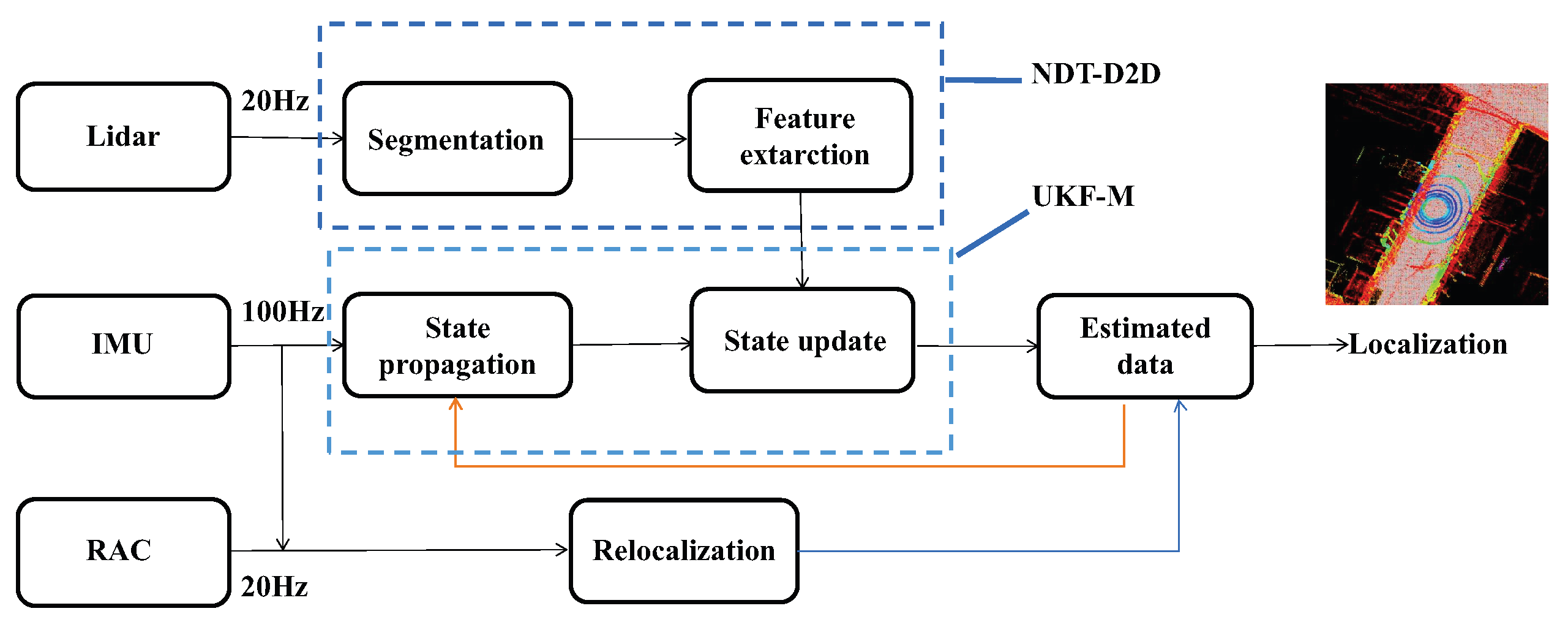
4. Multi-Sensor Data Fusion Framework

4.1. Definition of the Framework

The overall framework of this paper is illustrated in Figure 2. In this framework, the IMU serves as a source for predicting filtered states, while the 3D lidar provides precise observations through point cloud matching. Additionally, an RAC (Realtime Array Calibration) relocalization algorithm is designed to ensure the algorithm’s stability in challenging environments. Compensation mechanisms are established among multiple sensors such as point cloud distortion correction and global relocalization, which are detailed in Section 4.3.3.

4.2. Left-Invariant Measurements

Sensor observations are typically represented in the following form:

$$\begin{array}{c}\hfill y=h\left(x\right)+v\end{array}$$

(13)

where $h(.):G\to {\mathbb{R}}^k$ represents the observation equation and v is a Gaussian random noise term. By utilizing the general form in Equation (5), the generic representation of the measurement can be updated to

$$\begin{array}{c}\hfill Y=Xexp\left(v\right).\end{array}$$

(14)

Simultaneously, Equation (4) can undergo dynamic model transformation:

$$\begin{array}{c}\hfill X_n=X_{n-1}exp({\omega }_n+w_n),\end{array}$$

(15)

where ${\omega }_n$ represents the sensor input control information and $w_n$ is the Gaussian random noise term.

4.3. Manifold-Based Unscented Kalman Filter

The EKF framework typically relies on Gaussian assumptions and Taylor expansion to linearize models, thereby enabling derivation of the system’s probability distribution. On the other hand, the UKF approaches the problem by simulating a set of points to approximate the system’s underlying probability distribution. This addresses the issue faced in higher-order systems when using EKF, where the geometric expansion of Jacobian matrices leads to excessive utilization of computational resources.

To tackle this challenge, transforming the sigma points (the point set required for attitude estimation) generated by UKF from Euclidean space to a Riemannian manifold simplifies the calculation of more accurate robot poses. Performing the UT transformation within the manifold exploits the advantages of Lie groups while disregarding related lower-order terms, consequently reducing the overall system error. This technique contributes to more precise state estimation for the robot.

4.3.1. System Prediction

The a priori state of the robot’s overall system can be defined as follows.

$$\begin{array}{c}\hfill {\widehat{X}}_n=f\left({\widehat{X}}_{n-1},{\omega }_n\right)\end{array}$$

(16)

The former ${\widehat{X}}_{n-1}$ represents the state estimate from the previous time step. According to [29], predictions for the previous time step’s state can be made using the three-axis acceleration and three-axis angular velocity data from the IMU, eliminating the need to perform Unscented Transformation (UT), which approximate the Gaussian distribution using a certain number of parameters.

$$\begin{array}{c}\hfill \begin{array}{c}\lambda =({\alpha }^2-1)2q\\ W_c^j=\frac{1}{2\left(\lambda +2q\right)},j=1,\dots \dots ,4q\\ {\xi }_j=\pm \mathrm{col}\sqrt{\left(\lambda +d\right)p_{n-1}}),j=1,\dots \dots ,4q\end{array}\end{array}$$

(17)

When applying Unscented Transformation (UT) in robotics, it is common to select $\lambda =1$ to reduce the algorithm’s uncertainty. Here, W represents the weight term in the subsequent pose estimation and q represents the system’s state dimension. We select the parameter changes ${\xi }_i$ for the sigma points. Due to the state points transitioning into the manifold space, the selection of sigma points cannot follow the conventional approach. The sigma points can be updated as follows.

$$\begin{array}{c}\hfill X_n^j=f(\phi ({\widehat{X}}_{n-1},{\xi }_j),{\omega }_n)\end{array}$$

(18)

The covariance is computed in the tangent space. First, it is necessary to define the equivalent functions complementarily using the left-invariant and right-invariant properties, as defined in Equation (3). Additionally, we define the inverse transformation mapping from the Lie group to the Lie algebra ${\phi }^{-1}:logM\times M\in {}^d$.

$$\begin{array}{c}\hfill \begin{array}{c}{\phi }_{\widehat{x}}^{-1}\left(x\right)=log(\widehat{x}{x}^{-1}\left)\right(\mathrm{Right})\\ {\phi }_{\widehat{x}}^{-1}\left(x\right)=log(x^{-1}\widehat{x}\left)\right(\mathrm{left})\end{array}\end{array}$$

(19)

The covariance in the manifold-based form can be determined as follows.

$$\begin{array}{c}\hfill \sum _n=\sum _{j=1}^{2d+1}{W}_c^j{\phi }_{{\widehat{x}}_n}^{-1}\left(x_n^j\right){\left({\phi }_{{\widehat{x}}_n}^{-1}\left(x_n^j\right)\right)}^{\mathrm{T}}\end{array}$$

(20)

4.3.2. System Updating

In this approach, the results of point cloud matching serve as the observations. These results are obtained based on Equation (13), which takes input from both the point cloud map $S_{pt}$ and real-time 3D lidar point cloud data $H_{pt}$, satisfying the fundamental model described in Equation (15).

$$\begin{array}{c}\hfill Y_{input}=\left(\begin{array}{cc}R& P\\ 0& 1\end{array}\right)\in G\end{array}$$

(21)

Due to the incorporation of observations, the system state in the Lie algebra representation temporarily expands from ${\mathbb{R}}^{15}$ to ${\mathbb{R}}^{15+6}$.

By approximating the augmented portion with sigma points and applying the results to the original system state, we obtain a new set of sigma points $s{p}_n$ after incorporating observations. For the Lie algebra-based point set $s{p}_n$, the mean of the observation point set is calculated as shown below.

$$\begin{array}{c}\hfill \overline{sp}=\sum _{j=1}^{2d+1}{W}_c^{j}s{p}_j\end{array}$$

(22)

The observation covariance $P_{yy}$ and cross-covariance $P_{sp}$ are jointly obtained based on the mean of the observation point set $\overline{sp}$ and the mean of the observations $\overline{y}$:

$$\begin{array}{c}\hfill \begin{array}{c}{P}_{yy}={\displaystyle \sum _{j=1}^{2d+1}}{W}_c^j(y_j-\overline{y}){(y_j-\overline{y})}^{\mathrm{T}}\\ P_{sp}={\displaystyle \sum _{j=1}^{2d+1}}{W}_c^j(s{p}_j-\overline{sp}){(y_j-\overline{y})}^{\mathrm{T}}\end{array}\end{array}$$

(23)

where $y_j$ represents the approximation in Lie algebra form of the observation Y. However, in accordance with Equation (15), the general observation model can be transformed into the new form shown below.

$$\begin{array}{c}\hfill \begin{array}{c}{y}_j=log\left(XV\right)=log(exp\left(\xi \right)V)\\ y_j=\xi +v+o\left(\xi \right)\approx \xi \end{array}\end{array}$$

(24)

By applying the BCH (Baker–Campbell–Hausdorff) formula, it can be verified that transforming the sigma points into the Lie algebra for computation ensures the normality of the probability distribution and prevents the occurrence of outliers in the algorithm’s posterior results. The updating of the system’s state and covariance is similar to the standard Unscented Kalman Filter.

$$\begin{array}{c}\hfill \begin{array}{c}{\overline{X}}^{+}=\overline{X}exp\left({\displaystyle \sum _{j=1}^{2d+1}}{W}_c^j(y_j-\overline{y})\right)\\ P^{+}=P-P_{sp}{\left(P_{sp}{P}_{yy}^{-1}\right)}^{\mathrm{T}}\end{array}\end{array}$$

(25)

4.3.3. Design of Point Cloud Distortion Correction and Relocalization

During the motion of a robot, the lidar sensor cannot simultaneously capture a complete frame of point cloud data when the robot employs turning or other locomotion methods. As a result, the point cloud data may exhibit a degree of distortion. Because the sensor itself cannot perform distortion correction, IMU (Inertial Measurement Unit) information is required for specific correction and compensation. For systems equipped with high-frequency IMUs, only the time difference between two consecutive IMU data frames needs to be calculated (${\mathbf{R}}_d=\frac{t_i-t_{\mathrm{k}+1}}{t_k-t_{\mathrm{k}+1}}{\mathbf{R}}_o$) and interpolation is unnecessary. Integration of the angular velocity is achieved through the simplified process shown below.

$$\begin{array}{c}\hfill \begin{array}{c}{\mathbf{R}}_{x,y,z}^{\mathrm{t}}={\mathbf{R}}_{x,y,z}^{\mathrm{t}-1}+{\mathbf{A}}_{x,y,z}^{imu}\ast \mathsf{\Delta }t\end{array}\end{array}$$

(26)

For stable systems, relying solely on point cloud matching is insufficient. To ensure environmental stability in various conditions, fusion of multiple sensors is necessary. In this paper, we introduces an adaptive relocalization algorithm, Realtime Array Calibration (RAC), which addresses the reduction in point cloud matching performance when there are numerous similar feature points (see Algorithm 1).

Algorithm 1: Adaptive Relocalization Algorithm.

5. Experimental Design and Results

5.1. Experimental Environment and Setup

This section describes a series of experiments carried out to qualitatively and quantitatively analyze the localization framework proposed in this paper. The sensor suite that we used consisted of a combined handheld device comprising a depth camera (D435), a 16-line LiDAR sensor (Velodyne VLP-16), and an IMU (3DM-GX5). As depicted in Figure 3, this platform served as the sensor data input source for algorithm validation.

The geographical and point cloud structures are illustrated in Figure 4. The chosen experimental scene is surrounded by grassy areas, scattered trees, and moving vehicles. The roads exhibit irregularities, and the surrounding buildings often feature transparent glass elements. We anticipate that these nonstructured point clouds may pose a challenge to the localization system.

By reducing the reliance on robot odometry in most localization algorithms, the approach described in this paper enhances the algorithm’s overall versatility. Consequently, the algorithm presented here is equally applicable to a range of scenarios, including wheeled robots, legged robots, drones, and more.

The experimental platform utilizes the NVIDIA Jetson AGX Xavier (with eight-core ARM CPU, 64-bit architecture, 32 GB RAM, 32 GB storage, and a 512-core Volta GPU) as the upper-level computer, running Ubuntu 20.04 as the operating system, and uses the ROS (Robot Operating System) Noetic middleware for data handling.

5.2. Experimental Results

5.2.1. NDT-CUDA

In most cases, embedded upper-level computers use ARM chip architectures, which typically lack high computational performance. However, for larger maps, the amount of point cloud data needing to be handled is massive. Real-time point cloud matching consumes significant computational resources, which is not in line with the expectations of a reasonable localization system.

In our experiments, the NDT calculation thread was offloaded to the GPU; comparative experiments with field matching algorithms (Direct1, Direct7) were conducted to validate their performance. The point cloud map had a resolution of 0.2 m and two sets of parameters (0.1 m and 0.2 m) were selected for a downsampling comparison. The Direct7 matching algorithm performs more extensive field searches compared to Direct1, demanding more computational resources. In

Table 1. Performance evaluation of GPU-based localization.

Approaches	Dsmp (Map/m)	Dsmp (Lidar/m)	Search Method	CPU/%	Mem/Gb	Drift
NDT-P2D-CUDA	0.1	0.2	DIRECT7	114	1.28	No
	0.2	0.1	DIRECT7	87	0.88	No
	0.2	0.2	DIRECT7	103	0.88	Yes
	0.1	0.1	DIRECT7	100	1.78	No
NDT-D2D-CUDA	0.1	0.2	DIRECT7	92	1.28	No
	0.2	0.1	DIRECT7	79	0.88	No
	0.2	0.2	DIRECT7	105	1.08	No
	0.1	0.1	DIRECT7	95	0.88	No
NDT-OMP-CPU	0.1	0.2	DIRECT1	290.4	1.52	Yes
	0.2	0.1	DIRECT1	217	0.87	Yes
	0.2	0.2	DIRECT1	279.2	0.93	Yes
	0.1	0.1	DIRECT1	290.4	1.52	Yes

1. Dsmp stands for downsampling. 2. The parameters in bold in the table will be used in the overall framework.

, the performance of NDT-OMP with Direct7 is relatively poor, though it is not specifically recorded. The Drift parameter evaluates rotation offsets greater than 45° and translation distances exceeding one meter, serving as an indicator of the point cloud matching stability in the same environment.

The CUDA-based NDT-D2D algorithm exhibits efficient resource utilization and minimal increase in GPU memory usage, making it a resource-efficient choice.

5.2.2. Trajectory Comparison Results

To assess the performance of LIF-M in 3D environments, we conducted comparisons with different algorithms and frameworks that have been widely recognized and studied. These comparative frameworks were chosen to ensure the reasonableness and stability of LIF-M.

The compared frameworks included LIO-SAM [11], which is primarily optimization-based; LINS [14], which is based on IESKF, primarily derived from EKF; and a UKF localization framework operating in Euclidean space. The experiments were conducted using a handheld mapping device built on an AGX Xavier platform, with the navigation environment depicted in Figure 4 used for functional testing. The environment was approximately 100 m × 100 m in size, resembling a square, and had a significant number of terrain irregularities to challenge the algorithms, particularly in the upper region.

Based on the position output data and Figure 5d, it can be observed that the optimization-based methods tend to exhibit weaker precision and more drifted paths for localization in larger scenes. The overall trajectory suggests that filtering demonstrates certain advantages.

To ensure data uniformity across sensors, datasets of approximately 460 s, including LiDAR, IMU, and RAC data, were recorded using the rosbag functionality in ROS as the input source for the algorithms. During the recording process, the robot was maintained at a constant speed and encouraged to move in as straight a line as possible.

LINS improves the robot’s state information by iteratively generating new features using the estimates of the local frame and IESKF. This approach leads to superior performance in overall localization and stability in challenging environments. From Figure 5b,d, it can be inferred that LIF-M exhibits lower oscillations and higher accuracy to a certain extent, akin to LINS.

A comparative experiment was conducted between UKF and LIF-M regarding deviations during straight-line motion. Datasets of approximately 10 s were collected along a straight path and the yaw values were compared, as illustrated in Figure 6. LIF-M demonstrates smaller angular fluctuation during straight-line motion, with a maximum deviation of around 6°, less than the 10° oscillation error exhibited by UKF.

Analyzing the trajectory shown in Figure 5c, it can be observed that LIF-M’s position trajectory is smoother. This is attributed to its representation of sigma points in a group-like manner and calculations performed in the Lie algebra vector space, both of which offer advantages in terms of reducing disturbances and enhancing stability.

To clarify the comparison between algorithms, we calculated the absolute trajectory error (ATE) algorithm metrics using the Campus dataset (Figure 4). As shown in

Table 2. ATE translation error.

	UKF	LIO-SAM	LINS	LIF-M
Error/m	0.55	0.92	0.75	0.47

, LIF-M has a lower global error, helping to ensure operation in a variety of challenging environments.

We additionally incorporated the M2DGR dataset [30] crafted by Shanghai Jiao Tong University to complement the validation of nonstructured environments. The hardware we employed encompassed a Velodyne VLP-32C LiDAR, GNSS (Ublox M8T), and IMU (Handsfree A9, nine-axis), among others.

The M2DGR dataset contains a significant amount of forestry environments and irregular road surfaces (The bird’s-eye view of the point cloud is shown in Figure 7). We aimed to leverage these nonstructured features to challenge the tested systems.

The experiments involved a challenging section of road, comprising approximately 300 s of forestry road and around 100 s of lakeside steep slope road. When selecting specific paths in nonstructured environments and comparing the rotational offsets between LIF-M and UKF (Figure 8), it is evident that LIF-M exhibits superior stability with smoother variation curves, especially in conditions with dense foliage and reflective surfaces on lakeshores.

By constructing a three-dimensional visual representation of the test path (Figure 9), it is evident that LIF-M outperforms UKF in terms of system stability and algorithm accuracy in unstructured environments. This highlights how the utilization of the Lie group space enhances the robot’s perception capabilities in three-dimensional environments

5.2.3. Stability Experiment Analysis

For localization algorithms, stability is to a certain extent related to the maximum error within the relevant time. To further validate the performance of LIF-M, we carried out static error tests and dynamic error tests, with the results shown in

Table 3. Results of static performance testing.

Number	Point Position	Max Error/m
1	[−95.4, 19.2]	0.042
2	[−71.2, 39.4]	0.051
3	[0.0, −5.39]	0.055
4	[−10.2, −28.7]	0.031
5	[83.2, −39.3]	0.033
6	[59.7, −59.5]	0.024

and

Table 4. Results of dynamic performance testing.

Number	Path	Max Error/m
1	[−95.2, −31.1] −> [43.2, −101.2]	0.0243
2	[−115.1, −28.5] −> [53.2, −105.4]	0.01687
3	[84.1, −52.3] −> [67.3, 101.3]	0.00532
4	[2.35, 1.92] −> [−27.3, −56.2]	0.0482
5	[−59.3, 52.3] −> [79.79, −38.2]	0.0651
6	[−78.7, 50.24] −> [−114.5, −25.1]	0.0091

, respectively.

In the static error experiments, datasets of approximately 100 s were selected to test algorithm error in a scenario with no movement. Most of the data were clustered to obtain the reference origin, with the most distant point recorded as the static error point. The algorithm publishes the robot’s pose at a frequency of 10 Hz. For the circular area set used for static error calculation, enough points were obtained within 100 s to estimate the maximum error produced by the robot. According to the data in Table 3, the static error ranged from 0.03 m to 0.05 m, which is considered favorable for a versatile localization algorithm.

For the dynamic error experiments, datasets of approximately 50 s were selected, mostly involving straight-line motion tests. Quadratic regression was used to fit the absolute path of the state set. The maximum value of the dynamic error point was recorded as the point farthest from the reference path. For a moving robot, 50 s of attitude data is enough to generate a path to calculate algorithm stability under dynamic conditions. While more time may make the trajectory longer, it does not affect the actual error. According to the data in Table 4, the dynamic error ranged from 0.005 m to 0.06 m. There were variations in the velocities between different groups, leading to a relatively large deviation between the lower and upper bounds; however, the overall dynamic error meets the requirements of the localization system.

5.3. Discussion of the Issues

While the experimental results indicate that LIF-M exhibits superior performance, it is worth noting that in environments resembling terrain irregularities, such as the oscillations observed in the red trajectory in Figure 5a, noise in the z-axis can introduce fluctuations in the system. This represents a specific error in the three-dimensional manifold space; however, due to the uncertainties arising from the system’s left-invariant and right-invariant properties, this oscillation can quickly converge to stability.

6. Conclusions

This paper primarily addresses the issue of trajectory oscillations that may arise in Euclidean space filters, particularly when faced with increased noise and changing environmental characteristics. By introducing the concept of manifolds into the Unscented Kalman Filter (UKF) and extending the dimension of the groups, we present a three-dimensional manifold localization framework (LIF-M) tailored for unstructured environments. Furthermore, the system’s overall performance is enhanced through auxiliary relocalization and point cloud counter-distortion techniques.

In terms of localization performance, our approach bears similarities to the iterative error-based approach to Localization in Non-Structural environments (LINS), while exhibiting improved robustness against disturbances compared to the standard UKF. Our results underscore the crucial assistance that state updates in manifold space provide in attitude estimation.

Finally, it is apparent that the sensitivity of the algorithm on the z-axis plays a role in promoting the global localization of humanoid robots.

References

1. Batra, V.; Jadon, C.; Kumar, V. A Cognitive Framework on Object Recognition and Localization for Robotic Vision. In Proceedings of the 2020 Indo—Taiwan 2nd International Conference on Computing, Analytics and Networks (Indo-Taiwan ICAN), Rajpura, India, 7–15 February 2020; pp. 125–131. [Google Scholar] [CrossRef]
2. Dong, H.; Weng, C.-Y.; Guo, C.; Yu, H.; Chen, I.-M. Real-Time Avoidance Strategy of Dynamic Obstacles via Half Model-Free Detection and Tracking with 2D Lidar for Mobile Robots. IEEE/ASME Trans. Mechatron. 2021, 26, 2215–2225. [Google Scholar] [CrossRef]
3. Tang, X.; Yang, Q.; Xiong, D.; Xie, Y.; Wang, H.; Li, R. Improving Multiscale Object Detection with Off-Centered Semantics Refinement. IEEE Trans. Circuits Syst. Video Technol. 2022, 32, 6888–6899. [Google Scholar] [CrossRef]
4. Ruilan, G.; Zeyu, W.; Sitong, G.; Changjian, J.; Yu, Z. LFVB-BioSLAM: A Bionic SLAM System with a Light-Weight LiDAR Front End and a Bio-Inspired Visual Back End. Biomimetics 2023, 8, 410. [Google Scholar]
5. Huang, Y.H.; Lin, C.T. Indoor Localization Method for a Mobile Robot Using LiDAR and a Dual AprilTag. Electronics 2023, 12, 1023. [Google Scholar] [CrossRef]
6. Huang, J.H.; Junginger, S.; Liu, H.; Thurow, K. Correcting of Unexpected Localization Measurement for Indoor Automatic Mobile Robot Transportation Based on neural network. Transp. Saf. Environ. 2023. [Google Scholar] [CrossRef]
7. Sitompul, G.H.; Fikri, M.R.; Hadisujoto, I.B. Autonomous mobile robot localization using Markov decision algorithm. AIP Conf. Proc. 2023, 2646, 050023. [Google Scholar]
8. Xianjia, Y.; Qingqing, L.; Queralta, J.P.; Heikkonen, J.; Westerlund, T.; Rus, D. Cooperative UWB-Based Localization for Outdoors Positioning and Navigation of UAVs aided by Ground Robots. In Proceedings of the 2021 IEEE International Conference on Autonomous Systems (ICAS), Montreal, QC, Canada, 11–13 August 2021; pp. 1–5. [Google Scholar] [CrossRef]
9. Xu, Y.; Shmaliy, Y.S.; Chen, X.; Zhuang, Y. Extended Kalman/UFIR Filters for UWB-Based Indoor Robot Localization under Time-Varying Colored Measurement Noise. IEEE Internet Things J. 2023, 10, 15632–15641. [Google Scholar] [CrossRef]
10. Frosi, M.; Bertoglio, R.; Matteucci, M. On the precision of 6 DoF IMU-LiDAR based localization in GNSS-denied scenarios. Front. Robot. AI 2023, 10, 1064930. [Google Scholar] [CrossRef] [PubMed]
11. Wu, M.-H.; Yu, J.-C.; Lin, Y.-C. Study of Autonomous Robotic Lawn Mower Using Multi-Sensor Fusion Based Simultaneous Localization and Mapping. In Proceedings of the 2022 International Conference on Advanced Robotics and Intelligent Systems (ARIS), Taipei, Taiwan, 24–27 August 2022; pp. 1–4. [Google Scholar]
12. Ning, H.; Fenghua, H.; Yi, H.; Yu, Y. Graph-based observability analysis for mutual localization in multi-robot systems. Syst. Control Lett. 2022, 161, 105152. [Google Scholar]
13. Lv, Z.; Chen, T.; Cai, Z.; Chen, Z. Machine Learning-Based Garbage Detection and 3D Spatial Localization for Intelligent Robotic Grasp. Appl. Sci. 2023, 13, 10018. [Google Scholar] [CrossRef]
14. Lequn, C.; Englot, B.; Xiling, Y.; Chaolin, T.; Jinlong, S.; Nicholas, P.; Youxiang, C.; Kui, L.; Seung, L. Multisensor fusion-based digital twin for localized quality prediction in robotic laser-directed energy deposition. Robot. Comput.-Integr. Manuf. 2023, 84, 102581. [Google Scholar]
15. Shan, T.; Englot, B.; Meyers, D.; Wang, W.; Ratti, C.; Rus, D. LIO-SAM: Tightly-coupled Lidar Inertial Odometry via Smoothing and Mapping. In Proceedings of the 2020 IEEE/RSJ International Conference on Intelligent Robots and Systems (IROS), Las Vegas, NV, USA, 25–29 October 2020; pp. 5135–5142. [Google Scholar]
16. Ji, Z.; Sanjiv, S. LOAM: Lidar Odometry and Mapping in Real-time. Robot. Sci. Syst. 2014, 2, 1–9. [Google Scholar] [CrossRef]
17. Shan, T.; Englot, B. LeGO-LOAM: Lightweight and Ground-Optimized Lidar Odometry and Mapping on Variable Terrain. In Proceedings of the 2018 IEEE/RSJ International Conference on Intelligent Robots and Systems (IROS), Madrid, Spain, 1–5 October 2018; pp. 4758–4765. [Google Scholar]
18. Qin, C.; Ye, H.; Pranata, C.E.; Han, J.; Zhang, S.; Liu, M. LINS: A Lidar-Inertial State Estimator for Robust and Efficient Navigation. In Proceedings of the 2020 IEEE International Conference on Robotics and Automation (ICRA), Paris, France, 31 May–31 August 2020; pp. 8899–8906. [Google Scholar]
19. Julier, S.J.; Uhlmann, J.K. Unscented filtering and nonlinear estimation. Proc. IEEE 2004, 92, 401–422. [Google Scholar] [CrossRef]
20. Wu, K.; Zhang, T.; Su, D.; Huang, S.; Dissanayake, G. An invariant-EKF VINS algorithm for improving consistency. In Proceedings of the 2017 IEEE/RSJ International Conference on Intelligent Robots and Systems (IROS), Vancouver, BC, Canada, 24–28 September 2017; pp. 1578–1585. [Google Scholar]
21. Diemer, S.; Bonnabel, S. An invariant Linear Quadratic Gaussian controller for a simplified car. In Proceedings of the 2015 IEEE International Conference on Robotics and Automation (ICRA), Seattle, WA, USA, 26–30 May 2015; pp. 448–453. [Google Scholar]
22. Barfoot, T.D.; Furgale, P.T. Associating Uncertainty with Three-Dimensional Poses for Use in Estimation Problems. IEEE Trans. Robot. 2014, 30, 679–693. [Google Scholar] [CrossRef]
23. Tsao, S.H.; Jan, S.S. Observability analysis and consistency improvements for visual-inertial odometry on the matrix lie group of extended poses. IEEE Sens. J. 2020, 21, 8341–8353. [Google Scholar] [CrossRef]
24. Liu, H.; Yue, Y.; Liu, C. Automatic recognition and localization of underground pipelines in GPR B-scans using a deep learning model. Tunn. Undergr. Space Technol. 2023, 134, 104861. [Google Scholar] [CrossRef]
25. Zheng, S.; Liu, Y.; Weng, W.; Jia, X.; Yu, S.; Wu, Z. Tomato Recognition and Localization Method Based on Improved YOLOv5n-seg Model and Binocular Stereo Vision. Agronomy 2023, 13, 2339. [Google Scholar] [CrossRef]
26. Brossard, M.; Bonnabel, S.; Condomines, J.-P. Unscented Kalman filtering on Lie groups. In Proceedings of the 2017 IEEE/RSJ International Conference on Intelligent Robots and Systems (IROS), Vancouver, BC, Canada, 24–28 September 2017; pp. 2485–2491. [Google Scholar]
27. Brossard, M.; Barrau, A.; Bonnabel, S. A Code for Unscented Kalman Filtering on Manifolds (UKF-M). In Proceedings of the 2020 IEEE International Conference on Robotics and Automation (ICRA), Paris, France, 31 May–31 August 2020; pp. 5701–5708. [Google Scholar]
28. Forster, C.; Carlone, L.; Dellaert, F.; Scaramuzza, D. On-Manifold Preintegration for Real-Time Visual–Inertial Odometry. IEEE Trans. Robot. 2017, 33, 1–21. [Google Scholar] [CrossRef]
29. Barrau, A.; Bonnabel, S. Intrinsic Filtering on Lie Groups with Applications to Attitude Estimation. IEEE Trans. Autom. Control 2015, 60, 436–449. [Google Scholar] [CrossRef]
30. Yin, J.; Li, A.; Li, T. M2dgr: A multi-sensor and multi-scenario slam dataset for ground robots. IEEE Robot. Autom. Lett. 2021, 7, 2266–2273. [Google Scholar] [CrossRef]
Figure 1. Graphs of Lie group and Lie algebra spaces.
Applsci 13 11643 g001
Figure 2. Framework of the proposed localization algorithm.
Applsci 13 11643 g002
Figure 3. Multi-modal sensor platform.
Applsci 13 11643 g003
Figure 4. The ground scene as displayed using images of the Wish3d·Earth and the PCD map as displayed using Rviz software (version: 1.24.20).
Applsci 13 11643 g004
Figure 5. Trajectory comparison diagram (zoom in on different stages to obtain local detail map of (ad) diagram).
Applsci 13 11643 g005
Figure 6. Comparison of angle offset on a straight route.
Applsci 13 11643 g006
Figure 7. Unstructured experimental map from M2DGR (Multi-modal and Multi-scenario Dataset for Ground Robots).
Applsci 13 11643 g007
Figure 8. Partial three-dimensional trajectory comparison diagram.
Applsci 13 11643 g008
Figure 9. Yaw variation diagram of the robot’s forward path.
Applsci 13 11643 g009