Observation Capability Evaluation Model for Flood-Observation-Oriented Satellite Sensor Selection

Abstract

Satellite sensors are one of the most important means of collecting real-time geospatial information. Due to their characteristics such as large spatial coverage and strong capability for dynamic monitoring, they are widely used in the observation of real-time flood situation information for flood situational awareness and response. Selecting the optimum sensor is vital when multiple sensors exist. Presently, sensor selection predominantly hinges on human experience and various quantitative and qualitative evaluation methods. Yet, these methods lack optimization considering the flood’s spatiotemporal characteristics, such as different flood phases and geographical environmental factors. Consequently, they may inaccurately evaluate and select the inappropriate sensor. To address this issue, an innovative observation capability evaluation model (OCEM) is proposed to quantitatively pre-evaluate the performance of flood-water-observation-oriented satellite sensors. The OCEM selects and formulates various flood-water-observation-related capability factors and supports dynamic weight assignment considering the spatiotemporal characteristics of the flood event. An experiment involving three consecutive flood phase observation tasks was conducted. The results demonstrated the flexibility and effectiveness of the OCEM in pre-evaluating the observation capability of various satellite sensors across those tasks, accounting for the spatiotemporal characteristics of different flood phases. Additionally, qualitative and quantitative comparisons with related methods further affirmed the superiority of the OCEM. In general, the OCEM has provided a “measuring table” to optimize the selection and planning of sensors in flood management departments for acquiring real-time flood information.

1. Introduction

A flood is a type of complex meteorological disaster caused by heavy rainfall and typically characterized as sudden strong, wide coverage, and great damage [1,2], which can lead to emergencies, such as dams bursting [3], submerged farmland [4], and damaged houses [5]. Floods have always been the most frequent and severe natural disaster around the world. The accurate and timely monitoring of the flood water situational information (e.g., water level and submerged area) is vital to support flood response and management [6] in an effective manner. For this purpose, reliable sensors should be discovered and dispatched, which is the prerequisite for obtaining real-time high-quality flood water observation data [7,8].

Sensors can be roughly categorized as ground-based in situ sensors and space-based remote sensors [9,10]. Compared with in situ sensors, remote sensing satellite sensors can provide a lower cost and wider space-continuous observation, which is more robust and stable and easy to integrate with hydrological models [11,12]. Thus, remote sensing satellite sensors have been gaining more popularity in acquiring flood water observation data [13]. Currently, more than 900 Earth-observation-oriented orbiting satellites exist [14], and each satellite carries one or multiple sensors that are characterized by multidimensional observation capabilities. Observation capability is a new type of geographical phenomenon that can be used to understand the observation characteristics of sensors [15], which is composed of (1) static observation capability that is determined by the technical parameters, such as bands and spatial resolution, and (2) dynamic observation capability that varies with space and time, such as position and real-time observation area. However, there lacks an effective evaluation approach which can quantify the multidimensional satellite sensor observation capabilities considering the spatiotemporal characteristics (e.g., real-time weather and flood phases) of the flood event [11,16], leading to the unreliable selection of the optimum sensor. Therefore, quantifying the sensor observation capability under the consideration of spatiotemporal characteristics of the flood event is vital.

At present, two types of methods, qualitative- and quantitative-based evaluation methods, have been studied to evaluate the flood-water-observation-oriented satellite sensor observation capability.

Qualitative-based evaluation mainly includes two types of approaches, namely, experiment of application (EA) and capability analysis (CA). EA estimates the potentially qualified application of a satellite sensor by analyzing its past applications. Hu et al. [17] and Ban et al. [18] applied a Moderate Resolution Imaging Spectroradiometer in their flood water observation scenarios because its observation data are frequently utilized in flood submerged area extraction. Rahman and Thakur [19] produced the flood map through the analysis of time-series images taken by Synthetic Aperture Radar (SAR), having proved that SAR can observe the flood water. CA first identifies the flood water observation requirements and then determines whether a sensor qualifies by checking its multidimensional observation capabilities. Franci et al. [20] utilized GeoEye-1 to support flood susceptibility mapping because its spatial resolution meets the mapping requirement. The Tropical Rainfall Measuring Mission satellite is applied in real-time flood forecasting due to its high spatial and temporal resolutions [21,22]. Manson et al. [23] used a high-resolution SAR sensor to detect flooding in urban areas, owing to the ability of the SAR to penetrate clouds during both day and night. Li et al. argued that the GF-3 SAR satellite is suitable to observe ocean coasts, due to its full polarization, high spatial resolution, and wide imaging capabilities [24]. Although these approaches have realized the qualitative evaluation of satellite sensor observation capability, they cannot rank sensors due to the lack of accurate quantified values, leading to the failure in the optimum sensor selection.

Quantitative-based evaluation aims to construct the quantitative evaluation model or index, where multidimensional observation capabilities related to a specific flood scenario are considered and calculated, thereby ranking sensors on the basis of their quantified values. Chen et al. [25] utilized the observation data of a wide field-of-view sensor carried by the GF-1 satellite to invert the soil moisture and calculate various statistical indexes (e.g., mean absolute error and mean relative error) as the soil moisture observation capability of the sensor. Casella et al. [26] calculated the snowfall detection accuracy on the basis of Dual-frequency Precipitation Radar observation data to quantify its snowfall detection capability. On the basis of the convective precipitation data observed by x-band phased-array meteorological radar (XPAR), Wu and Liu [27] quantified the reflectivity, velocity difference, and sensitivity as observation capability evaluation indexes of XPAR. Yokota et al. [28] evaluated the capability of the existing GNSS-A system to detect long-term deformation and transient events based on observation data. However, they require existing observation data, and the spatiotemporal characteristics of the event are rarely considered. In other words, they cannot support the optimum sensor selection because the sensor observation capability cannot be pre-evaluated before observation. To pre-evaluate the observation capability in a quantitative manner, Chen and Zhang [29] proposed the dynamic observation capability index (DOCI) model to quantify the observation capability of optical satellite sensors, which can be dynamically applied in various emergencies, such as snowfall and oil spills. Liu et al. [30], Zhang et al. [31], and Chen et al. [32] constructed a series of observation-task-oriented indicators, such as time utilization ratio and observed profit ratio, to quantitatively pre-evaluate the sensor observation capability. Jin et al. [33] conducted a quantitative evaluation of the Earth observation satellite sensors’ multidimensional observation capabilities (e.g., satellite orbit and spatial resolution) to assess their potential in supporting sustainable development goals. Although these studies can quantitatively pre-evaluate the sensor observation capability to some extent, they are overly generic and not optimized on the basis of the spatiotemporal characteristics of the flood event, leading to failure in the optimum sensor selection.

To sum up, existing methods are inadequate in effectively supporting the quantitative pre-evaluation of satellite sensors’ observation capabilities considering the spatiotemporal characteristics of the flood event. This limitation has resulted in failures in selecting the optimal satellite sensors for flood monitoring. To address this issue, an observation capability evaluation model (OCEM) was developed. The OCEM has incorporated diverse flood-water-monitoring-oriented observation capability factors and dynamically adjusts to the spatiotemporal characteristics of each flood, allowing for a quantitative pre-assessment and ranking of different satellite sensors’ observation performance. The contributions of this research lie in innovatively proposing the OCEM, which accounts for the spatiotemporal nuances of flood events, facilitating the accurate quantitative measurement of satellite sensor observation capability. Secondly, it provides a practical “measuring table” for flood disaster management departments, enabling the effective and reliable selection of the most appropriate sensors for various flood scenarios.

2. Methodology

2.1. Description of Flood Observation Satellite Sensor Selection Problem

Assuming a flood disaster occurs in the middle reaches of the Yangtze River, as the flood emergency response department, the Changjiang Water Resource Commission (CWRC) needs to discover and dispatch a reliable satellite sensor for collecting real-time flood water observation data. The sensor planner first acquires a list of satellite sensors that can meet the fundamental observation requirements, such as observation space, time, and parameters. Their expected observation performance is evaluated and compared on the basis of their experiences or those aforementioned evaluation approaches [29,30,31], and the evaluated optimum sensor is selected. However, such a pattern ignores the spatiotemporal characteristics of the flood event, and how these characteristics could be considered and formulated is unclear. For example, an optical sensor might be pre-evaluated as the optimum at the early stage of a flood because it is the earliest one to respond, while it might not be the actual optimum one due to the heavy cloud cover; moreover, another sensor might be the optimum one at the late stage of a flood because it can obtain the highest-quality observation data. Consequently, the dispatched optimum sensor might work ineffectively due to the incomprehensive and inaccurate observation capability evaluation results.

In this situation, if a quantitative observation capability evaluation method that considers the spatiotemporal characteristics of a flood exists, the CWRC can obtain an accurate “measuring table” that reflects the expected observation performance of all sensors. This condition enables the sensor planner to select the actual optimum sensor for observing the more comprehensive and reliable flood water information.

2.2. OCEM Formalization

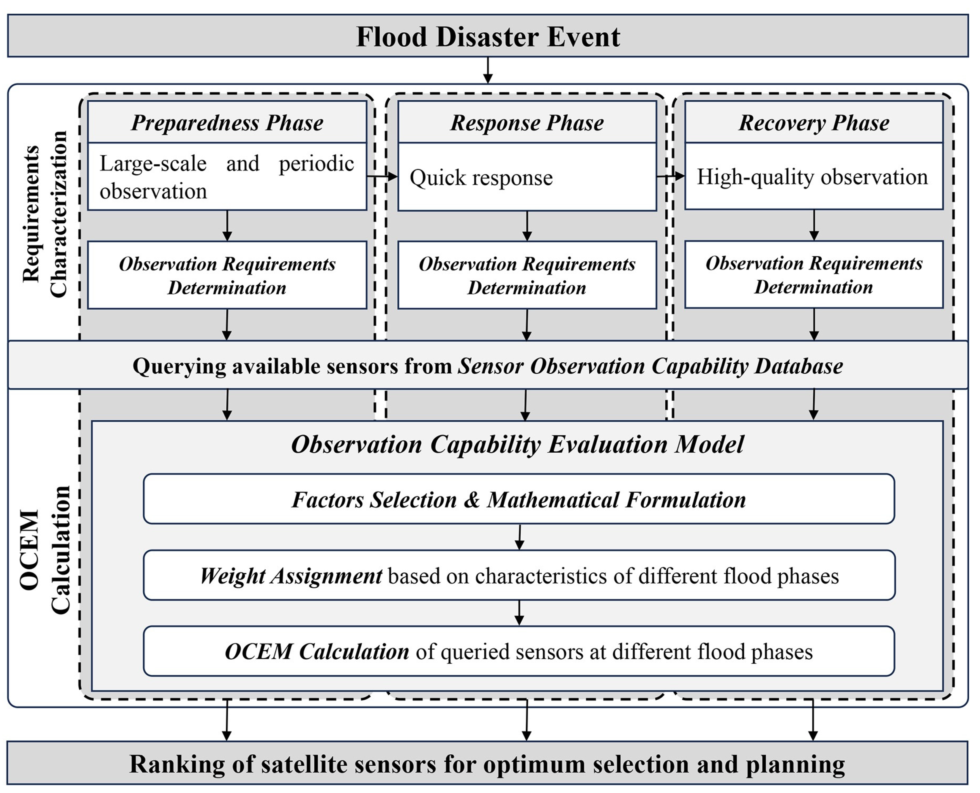
2.2.1. OCEM Framework

Given the abovementioned flood-water-observation-oriented optimum sensor selection problem, this study proposes the OCEM based on the analysis of flood-event-related studies [34,35,36]. Figure 1 shows the framework of the OCEM, which takes a flood disaster event as input and outputs a ranking of available satellite sensors by quantitatively evaluating their observation capabilities while accounting for the flood spatiotemporal characteristics of the flood. The framework consists of two components, requirements characterization and OCEM calculation, and the detail of each of them is as follows.

Requirements characterization: This aims to generate the flood observation requirements by considering the spatiotemporal characteristics of the flood event. Specifically, a flood disaster can be divided into three evolutionary phases [37], which are “preparedness”, “response”, and “recovery”. The preparedness phase usually requires large-scale and periodic observation, aiming to support flood detection and alerting by analyzing characteristics like water level rise and water changes. The response phase requires obtaining the flood water information as soon as possible due to the sudden strong and destructive flood water, thereby supporting the understanding of disaster situational information in time. The recovery phase requires the more high-quality observation data because the flood water state is relatively stable. Thus, the high-quality observation data are preferred to support the understanding of the detailed flood situation. Consequently, the observation requirements of each flood phase can be determined, which would include varying constraints on different observation capability factors, such as observation time, observation parameters, and spatial resolution.

OCEM calculation: This aims to quantitatively evaluate the expected observation performance of different satellite sensors using the proposed OCEM, which enables the optimal selection and planning of sensors for flood monitoring. To achieve this, as shown in Figure 1, we first mathematically formulate the OCEM by considering various flood-monitoring-related observation capability factors (e.g., observation space and spatial resolution). We then dynamically assign weights to these factors based on the spatiotemporal characteristics of the flood event (e.g., assigning a higher weight to spatial resolution during the recovery phase). Finally, we calculate the OCEM value for all satellite sensors queried from our constructed sensor observation capability database (SOCDB). Additionally, the rest of this chapter will focus on introducing the formalization and calculation of the OCEM.

2.2.2. OCEM Formulation

Equation (1) shows the mathematical formulation of the OCEM, which contains 10 observation capability factors related to flood water observation, and each ranges from 0 to 1. The quantified OCEM value can be calculated by applying linear and nonlinear operations on these factors.

$$\begin{gathered} OCEM=e^{(1+\alpha ·\mathrm{S}\mathrm{p}\mathrm{C}\mathrm{o})}\times e^{(1+\alpha ·\mathrm{T}\mathrm{h}\mathrm{C}\mathrm{o})}\times e^{(1+\alpha ·\mathrm{E}\mathrm{n}\mathrm{v})} \\ \times e^{{(1+\alpha ·(f}_1\times \mathrm{S}\mathrm{p}\mathrm{a}\mathrm{R}\mathrm{e}\mathrm{s}+f_2\times \mathrm{S}\mathrm{p}\mathrm{e}\mathrm{R}\mathrm{e}\mathrm{s}+f_3\times \mathrm{P}\mathrm{o}\mathrm{l}+f_4\times \mathrm{R}\mathrm{a}\mathrm{d}\mathrm{R}\mathrm{e}\mathrm{s}+f_5\times \mathrm{T}\mathrm{i}\mathrm{C}\mathrm{o}+f_6\times \mathrm{R}\mathrm{e}\mathrm{F}\mathrm{c}+f_7\times \mathrm{R}\mathrm{e}\mathrm{V}\mathrm{i}\left)\right)}. \end{gathered}$$

(1)

Table 1. Variables used in the OCEM and their descriptions.

Variable	Meaning
SpCo (spatial coverage)	The spatial coverage ratio of a sensor to the task area.
TiCo (time coverage)	The time coverage ratio of a sensor to the task time window.
ThCo (theme conformity)	The similarity between a sensor’s observation parameters and the task’s required parameters under a specific observation theme.
ReTi (response timeliness)	The response timeliness of a sensor to the task.
ReFc (revisit frequency)	The frequency of a sensor observing the task area within the task time window.
SpaRes (spatial resolution conformity)	The coincidence rate of a sensor’s spatial resolution to the task’s required one.
SpeRes (spectral resolution conformity)	The coincidence rate of a sensor’s spatial resolution to the task’s required one.
Pol (polarization mode conformity)	The coincidence rate of a sensor’s polarization resolution to the task’s required one.
RadRes (radiation resolution conformity)	The coincidence rate of a sensor’s radiation resolution to the task’s required one.
EnIm (environment impact)	The extent to which geographical environmental factors influence the observation quality.

shows the meaning of all the variables in the OCEM, all of which are selected and defined by considering the satellite sensor’s spatiotemporal validity, observation robustness, and observation quality. Specifically, SpCo, ThCo, and EnIm are decisive factors to the overall observation performance, whereas the seven other factors jointly determine the quality of the expected observation data. For example, a satellite sensor can definitely provide two times the amount of observation data if it can observe a two times larger area. Moreover, an assumption is made in terms of the linear relationships among these factors, that is, SpCo, ThCo, and EnIm are linearly independent, and the other seven factors are linearly correlated. Consequently, the OCEM is formulated as the multiplication of SpCo, ThCo, EnIm, and the linear weighted sum of the other seven factors.

However, a multiplication effect would emerge when the factor’s value is small. For example, 0.01 and 0.04 are extremely small, and the calculated OCEM values differ by a factor of four when multiplying by the two values. Intuitively, such an effect is extremely unreasonable and dangerous. Given this, the exponential method is applied to reduce such an effect, where $\alpha$ is an adjustable positive scaling factor (Equation (1)), and the tests show that it performs well when $\alpha =0.2$. Thus, a small factor value will not result in a large gap in the OCEM value, and a relatively large factor value can be accurately reflected. Notably, if the value of SpCo, ThCo, EnIm, or the last linear combination factor is equal to 0, the OCEM is equal to 0.

The weight vector $\mathit{f}=\{f_1,f_2,f_3,f_4,f_5,f_6,f_7\}({\sum }_{i=1}^7{f}_i=1,f_i\in (0,1\left)\right)$ can be set dynamically on the basis of the spatiotemporal characteristics of the flood event. For example, the weight of ReTi should be higher in the response phase. For this goal, an appropriate weight assignment method should be adopted, and the analytic hierarchy process (AHP) [33] was selected. A more detailed illustration is elaborated in Section 2.3.

2.3. OCEM Solving

In Figure 2, the solving workflow of the OCEM is represented, which mainly includes the following two steps.

First, as depicted in Figure 1, the available satellite sensors would be queried from the SOCDB based on the observation requirements specific to one particular flood phase. Then, the detail value of each observation capability factor (e.g., SpCo) of those queried sensors would be calculated. The detailed calculation of those factors will be introduced in Section 2.3.1.

Second, after calculating the observation capability factor values, the weights of those seven linearly correlated factors would be determined using the AHP method. Consequently, the OCEM value of all the sensors can be evaluated, and the detailed weight assignment procedure will be introduced in Section 2.3.2.

2.3.1. Calculation of Observation Capability Factors

This section presents the detailed calculations of these observation capability factors.

• SpCo: This can be calculated by using Equation (2), where $S_{Cover}$ is the sensor’s observation area and $S_{Task}$ is the whole task area.

  $$SpCo=\left\{\begin{array}{c}{S}_{Cover}/S_{Task},S_{Cover}\cap S_{Task}\ne \varnothing \\ 0,S_{Cover}\cap S_{Task}=\varnothing \end{array}\right.$$

  (2)
• TiCo: This can be calculated by using Equation (3), where $T_{Cover}$ is the sensor’s time window and $T_{Task}$ is the task’s required time window.

  $$TiCo=\left\{\begin{array}{c}{T}_{Cover}/T_{Task},T_{Cover}\cap T_{Task}\ne \varnothing \\ 0,S_{Cover}\cap S_{Task}=\varnothing \end{array}\right.$$

  (3)
• ThCo: This can be calculated by using Equations (4) and (5), where $w_i$ is the relevance degree of one specific observation parameter (e.g., land cover) to the flood, and $N$ is the number of the task’s required observation parameters. The relevance degrees are quantified into six values, which are sourced from the Observing System Capability Analysis and Review Tool (https://space.oscar.wmo.int/instruments (accessed on 1 September 2023)) released by the World Meteorological Organization.

  $$ThCo={\sum }_{i=1}^N{w}_i/N$$

  (4)

  $$w=\left\{\begin{array}{c}1,\mathit{primary}\\ 0.8,\mathit{high}\\ 0.6,\mathit{medium}\\ 0.4,\mathit{useful}\\ 0.2,\mathit{marginal}\\ 0,\mathit{else}\end{array}\right.$$

  (5)
• ReTi: This can be calculated by using Equation (6), where $T_{start}$ and $T_{end}$ are the start time and end time of the task, and $T$ is the time when the sensor can respond to the task.

  $$\mathit{ReTi}=(T_{end}-T)/(T_{end}-T_{start})$$

  (6)
• ReFc: This can be calculated by using Equation (7), where ${Rf}_i$ is the frequency of ${\mathrm{s}\mathrm{e}\mathrm{n}\mathrm{s}\mathrm{o}\mathrm{r}}_{\mathrm{i}}$, and a higher frequency can result in a better observation performance theoretically.

  $$\mathit{ReFc}={Rf}_i/\sqrt[2]{{\sum }_i{{Rf}_i}^2}$$

  (7)
• Observation quality: Observation quality is composed of four observation capability factors, namely, SpaRes, RadRes, SpeRes, and Pol. Each sensor only contains three of them because SpeRes only exists in optical sensors and Pol only exists in microwave sensors. Their detailed meanings and calculations are as follows:

  (1)

  SpaRes

  This refers to the size of one pixel on the ground, which determines how detailed a satellite image is [38]. SpaRes can be calculated by using Equation (8), where ${Spa}_{task}$ is the task’s required spatial resolution, and ${Spa}_i$ is the spatial resolution of ${\mathrm{s}\mathrm{e}\mathrm{n}\mathrm{s}\mathrm{o}\mathrm{r}}_{\mathrm{i}}$.

  $$SpaRes=\left\{\begin{array}{c}{Spa}_{task}/{Spa}_i,{Spa}_i\ge {Spa}_{task}\\ 1,{Spa}_i<{Spa}_{task}\end{array}\right.$$

  (8)

  (2)

  RadRes

  This reflects the capability of the sensor to recognize subtle changes in flood water radiation energy, which is represented by the radiometric quantization value of each image pixel [39]. RadRes can be obtained by using Equation (9), where ${Rad}_i$ is the radiometric quantization value of ${\mathrm{s}\mathrm{e}\mathrm{n}\mathrm{s}\mathrm{o}\mathrm{r}}_{\mathrm{i}}$, and ${Rad}_{task}$ is the task’s required radiometric quantization value. A higher radiometric quantization value results in a better observation performance.

  $$RadRes=\left\{\begin{array}{c}{Rad}_i/{Rad}_{task},{Rad}_i<{Rad}_{task}\\ 1,{Rad}_i\ge {Rad}_{task}\end{array}\right.$$

  (9)

  (3)

  SpeRes

  This reflects the capability of the sensor to recognize spectral features of ground objects [40], and a higher spectral resolution (smaller wavelength interval) facilitates better observation of complex flood scenarios, such as flood water, vegetations, and houses. SpeRes can be calculated by using Equation (10), where ${Spe}_{least}$ is the task’s required spectral resolution, $r_1$ is the task’s required wavelength range, $r_2$ is the wavelength range of the sensor, and $∆\left(r_1\cap r_2\right)$ is the wavelength range intersection of the task and sensor.

  $$SpeRes=\left\{\begin{array}{c}0,∆\left(r_1\cap r_2\right)=0\\ \begin{array}{c}{Spe}_{least}/∆(r_1\cap r_2),∆(r_1\cap r_2)\ge {Spe}_{least}\\ 1,∆(r_1\cap r_2)<{Spe}_{least}\end{array}\end{array}\right.$$

  (10)

  (4)

  Pol

  Different polarization modes cause different observation performance, for example, like polarization is more suitable for flood water identification when compared with cross-polarization [41,42], HH polarization is more effective than HV and VV polarization in recognizing the inundation area [43], and alternating polarization with co-polarization and cross-polarization is superior in flood mapping [44]. Consequently, on the basis of the review and analysis of related studies [43,45], Equation (11) is constructed to calculate Pol.

  $$Pol=\left\{\begin{array}{c}0.2,\mathit{VV}\\ 0.4,\mathit{VV}/\mathit{VH}\mathit{or}\mathit{HV}\mathit{or}\mathit{VH}\\ 0.6,\mathit{HH}\mathit{or}\mathit{HH}/\mathit{VV}\\ 0.8,\mathit{HH}/\mathit{HV}\\ 1,\mathit{HH}/\mathit{HV}/\mathit{VV}/\mathit{VH}\end{array}\right.$$

  (11)

• EnIm: A flood event is always accompanied by bad weather (e.g., heavy rainfall and thick clouds), which can have a great impact on satellite sensors. Geographical environmental factors, such as atmospheric refraction and topography, also influence the observation quality to some extent [42]. However, the impacts caused by atmospheric refraction or topography can be reduced or eliminated by using some existing mathematical approaches and physical models [46,47]. The thick clouds can only be reduced by using external satellite images or ground observations [48,49], which conflicts with the goal of planning sensors to acquire observation data.

Given the above analysis, this study only considers the impact caused by cloud cover, and EnIm can be calculated by using Equation (12), where Cl is the value of cloud cover. The EnIm of a microwave sensor is 1 because it is barely affected by cloud cover.

$$EnIm=\left\{\begin{array}{c}1-Cl,\mathit{optical}\\ 1,\mathit{microwave}\end{array}\right.$$

(12)

2.3.2. Weight Assignment of Observation Capability Factors

As described in Section 2.2.2, the weight vector $\{f_1,f_2,f_3,f_4,f_5,f_6,f_7\}$ for TiCo, ReTi, ReFC, SpaRes, SpeRes, Pol, and RadRes is determined dynamically using the AHP method. The AHP method is a subjective multi-criteria decision-making tool widely used in various fields for its structured approach to resolving complex problems. It allows decision makers to address complex decisions by breaking them down into a hierarchical structure. The procedure for assigning weights to those factors using AHP is as follows.

Establishing hierarchical structure: This involves creating a three-level hierarchical structure, including the main objective, criteria influencing the objective, and alternatives. In this study, the main objective is to quantitatively evaluate the satellite sensor’s observation capability during a specific flood phase. The criteria are those seven observation capability factors, and alternatives are the queried available satellite sensors.

Pairwise Comparison: The decision maker needs to perform pairwise comparisons for each criterion. The Saaty scaling method [50] is commonly used to quantify the relative importance between factors (

Table 2. Fundamental scale of absolute numbers.

Intensity of Importance	Definition	Explanation
1	Equal importance	Two activities contribute equally to the object
2	Weak or slight
3	Moderate importance	Experience and judgment favor slightly one activity over another
4	Moderate plus
5	Strong importance	Experience and judgment strongly favor one activity over another
6	Strong plus
7	Very strong or demonstrated importance	An activity is favored very strongly over another; its dominance is demonstrated in practice
8	Very, very strong
9	Extreme importance	The evidence favoring one activity over another is of the highest possible order of affirmation

). For example, SpaRes may be rated a 7 in terms of ReTi during the recovery phase. As a result, the pairwise comparison between all criteria can be represented as a matrix $A$ (Equation (13)), where each element $a_{ij}$ corresponds to the comparison result between the $i$-th criterion and $j$-th criterion.

$$A={\left(a_{ij}\right)}_{6\times 6}=\left[\begin{array}{cc}\begin{array}{cc}{a}_{11}& a_{12}\\ a_{21}& a_{22}\end{array}& \begin{array}{cc}\dots & a_{16}\\ \dots & a_{26}\end{array}\\ \begin{array}{cc}⋮& ⋮\\ a_{61}& a_{62}\end{array}& \begin{array}{cc}\ddots & ⋮\\ \dots & a_{66}\end{array}\end{array}\right]$$

(13)

Calculation of Relative Weights: This process calculates the weight of all criteria (factors) based on the matrix $A$. First, the maximum eignvalue ${\lambda }_{max}\in \mathbb{R}$ and its corresponding eignvector $e=[v_1,v_2,v_3,v_4,v_5,v_6,v_7]$ of $A$ should be calculated. Then, the consistency test is performed using Equation (14), where $n$ is number of criteria and $RI$ is a parameter that requires looking up in the table [50]. If the consistency test does not pass ($CR\le 0.10$), $A$ should be modified until the consistency test passes. Notably, the eignvector $e$ should be normalized to ensure that the sum of its elements equals 1.

$$CR=\frac{{\lambda }_{max}-n}{\left(n-1\right)\times RI}$$

(14)

3. Flood-Water-Observation-Oriented Satellite Sensor Selection Experiment

3.1. Flood Event and Observation Task Requirements

A heavy rainfall occurred in Henan Province, China, during 18 July and 21 July 2021, causing severe flood disasters, such as landslides and mudslides. In this flood disaster, 302 people lost their lives, 50 people were missing, more than 580,000 hectares of farmland were affected, and the economic loss was estimated to be approximately USD 18 billion [51]. This study selects this flood disaster as the background to conduct the flood-water-observation-oriented satellite sensor selection experiment, and Figure 3 shows the selected study area at longitude $111.5°\mathrm{W}–115°\mathrm{W}$ and $33.5°\mathrm{N}–36°\mathrm{N}$.

As shown in

Table 3. Observation requirements of the constructed three observation tasks.

Order	Phases	Time Window	Characteristics	Spatial Resolution	Spectral Resolution	Radiometric Resolution	Polarization Mode	Observation Parameters
1	Preparedness	13 July 0:00– 16 July 0:00	Large-scale and periodic observation	30 m	0.07 Micrometer (optical)	12 bits (radiometric quantization)	HH (microwave)	Land cover Precipitation intensity at surface (liquid or solid) Accumulated precipitation (over 24 h)
2	Response	19 July 0:00–24:00	Quick response	10 m
3	Recovery	23 July 0:00–24:00	High-quality observation	1 m

, three flood water observation tasks were constructed, corresponding to the three flood phases, and the detailed observation requirements were characterized and represented under the consideration of spatiotemporal characteristics of the three phases. For example, the spatial resolution requirement increased from 30 m to 1 m as the flood evolved.

3.2. Available Sensor Resources

By taking the spatiotemporal observation requirements of these three observation tasks as the query input, the SOCDB successfully discovered 16, 15, and 14 sensors, respectively (

Table 4. Overview of the available satellite sensors for the three observation tasks.

Flood Observation Task	#Available Optical Sensor	#Available Microwave Sensor
Preparedness phase	13	3
Response phase	13	2
Recovery phase	12	2

). More detailed observation capability information on these sensors can be found at http://www.bigdatasensing.cn/ocem/ (accessed on 1 October 2023).

3.3. OCEM Calculation for Supporting Satellite Sensor Selection

In accordance with the OCEM solving workflow depicted in Section 2.3, a three-step calculation is required for each observation task. First, the values of all 10 observation capability factors were calculated by using the calculation methods introduced in Section 2.2. Second, the weights of the seven linearly correlated factors were calculated by using the AHP. Third, the OCEM value of each sensor was calculated on the basis of the results of the former two steps, thus supporting the ranking and selection of the optimum sensor.

3.3.1. Calculation and Results of Observation Capability Factors

Despite the obtained observation capability information of these obtained sensors (Section 3.2), real-time weather information was further queried from WWO in 1 h resolution, and the observation parameter relevance information was queried from OSCAR accordingly to calculate the values of the 10 observation capability factors.

The values of all observation capability factors were calculated with respect to each observation task, which are represented in

Table 5. Values of the observation capability factors of each satellite sensor in the preparedness-phase task.

Sensor Type	Satellite Sensor	SpCo	ThCo	EnIm	SpaRes	SpeRes	Pol	RadRes	TiCo	ReTi	ReFc
Optics	Worldview 4_SpaceView-110	0.2057	0.2667	0.2600	1	1	/	1	0.2607	0.6153	0.2500
	Ziyuan1-02C_HRPC-2	0.4529	0	0.5400	1	0		1	0.2731	0.8539	0.2500
	KazEOSat-1_NAOMI (KazEOSat)	0.4836	0.2667	0.4700	1	1		1	0.2980	0.8449	0.2500
	RapidEye-1_REIS	0.3462	0.2667	0.4400	1	1		1	0.2731	0.5213	0.2500
	GeoEye-1_GIS	0.4081	0.2667	0.4700	1	1		1	0.2731	0.8413	0.2500
	SSOT_NAOMI(SSOT)	0.3771	0.2667	0.4700	1	1		1	0.2731	0.8437	0.2500
	Kompsat-2_MSC-Multi-Spectral Camera	0.4232	0.2667	0.3800	1	1		1	0.2855	0.5346	0.2500
	RapidEye-2_REIS	0.1573	0.2667	0.2500	1	1		1	0.1241	0.1893	0.2500
	Gaofen9_PMS-2	0.0734	0.2667	0.2100	1	1		1	0.0497	0.3547	0.2500
	Jilin-1_PMS-2	0.0891	0.2667	0.6100	1	1		1	0.0621	0.8624	0.2500
	Skysat-7_Skysat	0.2694	0.2667	0.2200	1	1		1	0.2607	0.6928	0.2500
	Gaofen-1-03_PMS	0.3846	0.2667	0.4700	1	1		1	0.2731	0.8411	0.2500
	Skysat-14_Skysat	0.2697	0.2667	0.5400	1	1		0.7500	0.2607	0.8496	0.2500
SAR	COSMO-Skymed 3_SAR-2000	0.3596	0.2000	1	1	/	0.8000	1	0.2607	0.9174	0.2500
	COSMO-Skymed 4_SAR-2000	0.3941	0.2000	1	1		0.8000	1	0.2855	0.7432	0.2500
	Coriolis_WindSat	0.5061	0.2667	1	1		0.8000	1	0.2855	0.2373	0.2500

,

Table 6. Values of the observation capability factors of each satellite sensor in the response-phase task.

Sensor Type	Satellite Sensor	SpCo	ThCo	EnIm	SpaRes	SpeRes	Pol	RadRes	TiCo	ReTi	ReFc
Optics	Worldview4_SpaceView-110	0.2045	0.2667	0.0300	1	1	/	1	0.2510	0.8414	0.2582
	Worldview2_WV110	0.4909	0.2667	0.0500	1	1		1	0.2869	0.5280	0.2582
	Kompsat-2_MSC—Multi-Spectral Camera	0.4245	0.2667	0	1	1		1	0.2749	0.6091	0.2582
	KazEOSat-2_KEIS	0.3742	0.2667	0	1	1		1	0.2630	0.0403	0.2582
	SkySat-2_SkySat	0.2232	0.2667	0	1	1		1	0.1554	0.1681	0.2582
	Worldview3_WV110	0.3887	0.2667	0	1	1		1	0.2749	0.0580	0.2582
	Pléiades HR1A_HiRI	0.4350	0.2667	0.0500	1	1		1	0.2749	0.5253	0.2582
	Ziyuan1-02C_HRPC-2	0.4927	0	0.0200	1	0		0.7500	0.2869	0.5664	0.2582
	Kompsat-3_AEISS	0.4269	0.2667	0.0900	1	1		1	0.2749	0.4361	0.2582
	Resurs-P1_ShMSA-VR	0.1671	0.2667	0.0200	0.8333	1		1	0.1554	0.5729	0.2582
	DubaiSat-2_HiRAIS	0.3615	0.2667	0	1	1		1	0.2630	0.6138	0.2582
	Gaofen-1-04_PMS	0.4049	0.2667	0.0700	1	1		1	0.2630	0.4619	0.2582
	Skysat-14_Skysat	0.2692	0.2667	0	1	1		1	0.2510	0.0681	0.2582
SAR	COSMO-Skymed1_SAR-2000	0.3771	0.2000	1	1	/	0.8000	1	0.2630	0.7607	0.2582
	Sentinel1A_SAR-C	0.4525	0.1333	1	1		0.8000	1	0.2869	0.7175	0.2582

and

Table 7. Values of the observation capability factors of each satellite sensor in the recovery-phase task.

Sensor Type	Satellite Sensor	SpCo	ThCo	EnIm	SpaRes	SpeRes	Pol	RadRes	TiCo	ReTi	ReFc
Optics	SkySat-1_SkySat	0.3547	0.2667	0.0500	1	1	/	1	0.2841	0.5304	0.2673
	DubaiSat-2_HiRAIS	0.3568	0.2667	0.2200	1	1		1	0.2841	0.1480	0.2673
	UK-DMC-2_SLIM6	0.3945	0.2667	0.0600	0.0455	0		1	0.2841	0.7429	0.2673
	Haiyang1C_CZI	0.1849	0.2667	0.0500	0.0040	1		1	0.1162	0.5325	0.2673
	Alsat2B_NAOMI	0.4210	0.2667	0.0200	0.4000	1		1	0.2970	0.5491	0.2673
	SkySat-13_SkySat	0.2524	0.2667	0.2100	1	1		1	0.2583	0.9386	0.2673
	SkySat-11_SkySat	0.2687	0.2667	0.1100	0.0008	0		1	0.2712	0.4215	0.2673
	Worldview3_WV110	0.3716	0.2667	0.0500	1	1		1	0.2841	0.5337	0.2673
	Skysat-5_SkySat	0.3068	0.2667	0.2400	1	1		1	0.2841	0.0804	0.2673
	SkySat-6_SkySat	0.1549	0.2667	0.2400	1	1		1	0.1550	0.0802	0.2673
	Landsat7_ETM+	0.0010	0.3333	0.1200	0.0667	11		1	0.2841	0.7657	0.2673
	RapidEye-2_REIS	0.3537	0.2667	0.2500	0.1538			1	0.2841	0.0953	0.2673
SAR	COSMO-Skymed3_SAR-2000	0.3775	0.2000	1	1	/	0.8000	1	0.2841	0.7607	0.2673
	Sentinel1B_SAR-C (Sentinel-1)	0.4336	0.1333	1	0.2500		0.8000	1	0.2970	0.2474	0.2673

. The satellite sensor column records the name of each satellite and its onboard sensor.

3.3.2. Weights Calculation and Results

Followed by the procedure of utilizing the AHP to calculate the weights of the seven observation capability factors, three relationship matrices were constructed on the basis of considering the spatiotemporal characteristics of the three observation tasks.

Table 8. Weight calculation result of the preparedness-phase task.

	ReTi	TiCo	ReFc	SpaRes	SpeRes/Pol	RadRes	Weight
ReTi	1	1/5	1/9	1/3	1/3	1/3	0.032
TiCo	5	1	1/5	5	5	5	0.236
ReFc	9	5	1	7	7	7	0.534
SpaRes	3	1/5	1/7	1	1	1	0.066
SpeRes/Pol	3	1/5	1/7	1	1	1	0.066
RadRes	3	1/5	1/7	1	1	1	0.066
${\lambda }_{max}$ = 6.340, CR = 0.055 < 0.1

,

Table 9. Weight calculation result of the response-phase task.

	ReTi	TiCo	ReFc	SpaRes	SpeRes/Pol	RadRes	Weight
ReTi	1	7	9	5	5	5	0.514
TiCo	1/7	1	3	1/3	1/3	1/3	0.057
ReFc	1/9	1/3	1	1/5	1/5	1/5	0.030
SpaRes	1/5	3	5	1	1	1	0.133
SpeRes/Pol	1/5	3	5	1	1	1	0.133
RadRes	1/5	3	5	1	1	1	0.133
${\lambda }_{max}$ = 6.190, CR = 0.031 < 0.1

and

Table 10. Weight calculation result of the recovery-phase task.

	ReTi	TiCo	ReFc	SpaRes	SpeRes/Pol	RadRes	Weight
ReTi	1	2	3	1/5	1/5	1/5	0.067
TiCo	1/2	1	2	1/7	1/7	1/7	0.042
ReFc	1/3	1/2	1	1/9	1/9	1/9	0.027
SpaRes	5	7	9	1	1	1	0.288
SpeRes/Pol	5	7	9	1	1	1	0.288
RadRes	5	7	9	1	1	1	0.288
${\lambda }_{max}$ = 6.051, CR = 0.008 < 0.1

show the matrices. As shown in Table 8, ReTi is more important than other factors in the response-phase task because all values are greater than one.

On the basis of these constructed matrices, the consistency tests were conducted, and the results are shown in the three tables. All consistency tests passed because all the CR values are less than 0.1. Their maximum eigenvalues ${\lambda }_{max}$ and corresponding eigenvectors (weights) are represented.

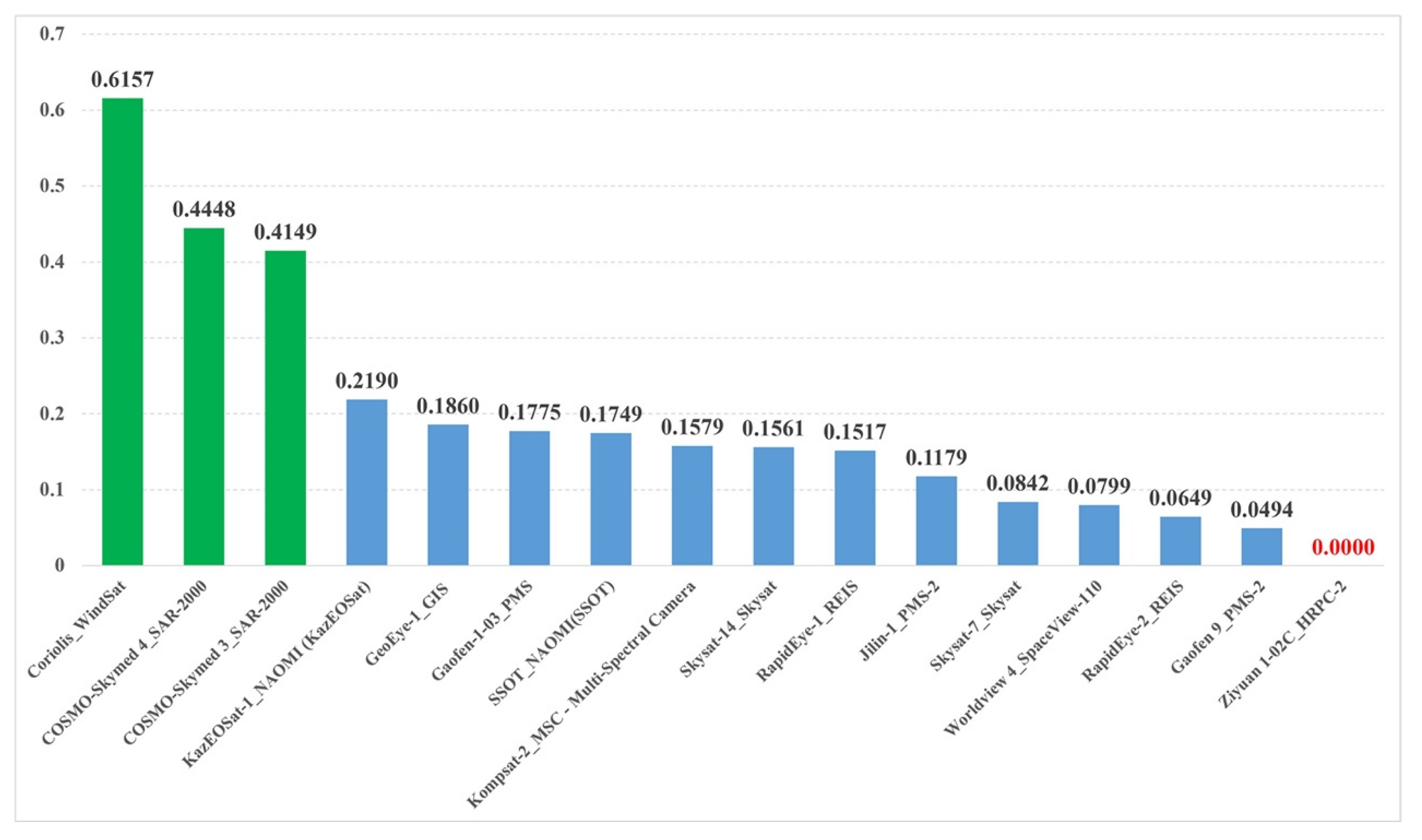
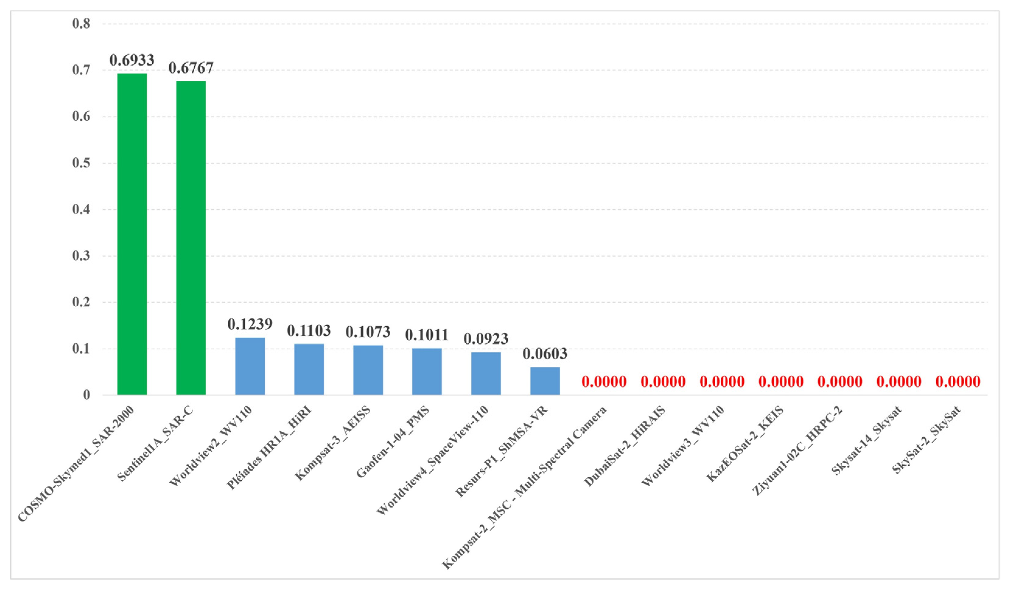
3.3.3. OCEM Calculation and Results

On the basis of the results of the former two subsections, the OCEM values of the satellite sensors of different observation tasks were calculated using Equation (1).

The OCEM calculation results of the three observation tasks are represented in Figure 4, Figure 5 and Figure 6, respectively. Moreover, the OCEM values for each task are standardized and represented in descending order.

As shown in Figure 4, the three microwave sensors were ranked as the top three in the preparedness-phase task, where the WindSat sensor carried by Coriolis ranked first, and the SAR-2000 sensor ranked second and third. The NAOMI sensor carried by KazEOSat-1 ranked first among the optical sensors, and the HRPC-2 sensor carried by Ziyuan 1-02C has an OCEM value of 0 because its ThCo value is 0. In terms of the response-phase task, the two microwave sensors were ranked as the top two (Figure 5), where the SAR-2000 sensor ranks first. Notably, Ziyuan 1-02C appears again and has an OCEM value of 0 for the same reason, and the other six sensors have an OCEM value of 0 due to the 100% cloud cover (EnIm = 0). Similarly, the only two existing microwave sensors ranked as the top two in the recovery-phase task, and the top one is SAR-2000 (Figure 6). Compared with the former two tasks, no sensor with an OCEM value of 0 was found. Based on the rankings shown in the three figures, the sensor planner should be able to select the optimum sensor to observe the flood water effectively.

4. Discussion

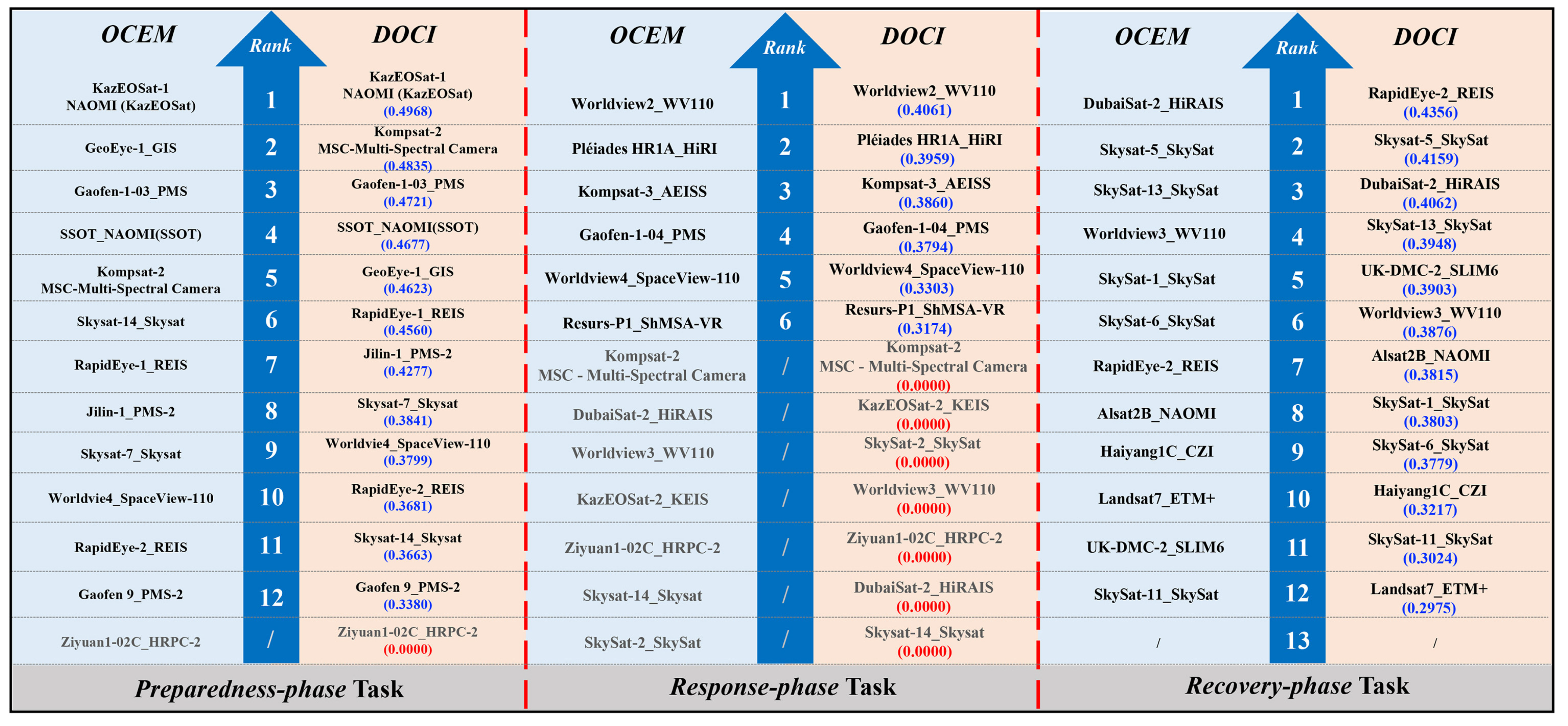
4.1. Supporting the Optimum Satellite Sensor Selection for Flood Observation

The experiment constructed three flood water observation tasks corresponding to the three evolutionary flood phases, and 16, 15, and 14 satellite sensors were discovered, evaluated, and ranked by utilizing the proposed OCEM to quantify their expected observation performances. The OCEM was effective in accurately quantifying the satellite sensor observation capability with spatiotemporal characteristics of the flood event considered, enabling the optimal selection of the flood-observation-oriented sensor, thereby supporting the real-time acquisition of flood observation information.

Taking the OCEM results of the preparedness-phase task (Figure 4) as an example, the results show that the three microwave sensors ranked the highest. As shown in Table 5, their high ranking is mainly because they are unaffected by clouds, whereas other optical sensors are greatly affected. Specifically, their EnIm values are 1, indicating that they have larger valid observations than optical sensors. Therefore, the proposed OCEM is more effective and accurate in practical application because it considers the impact of a real-time environmental influential factor (cloud cover). For example, six optical sensors with an OCEM value of 0 in the response-phase task (Figure 5) were found because their EnIm values are 0 (Table 6), indicating that optical sensors are completely unusable.

Benefiting from the flexible weight adjustment mechanism, the weights of the linearly correlated factors can be set dynamically on the basis of the spatiotemporal characteristics of a specific flood phase. Taking the recovery-phase task as an example, it prefers the sensor that can obtain high-quality observation data. As shown in Table 10, the weights of observation quality factors, SpaRes, SpeRes, and RadRes, account for 86.4% of the weight in total, and the three other factors only take up 13.6%, which complies with the high-quality observation requirement. Figure 6 shows a distinctive drop between NAOMI and CZI. As shown in Table 7, the optical sensors on the left of the drop have SpaRes values greater than 0.1, and sensors on the right of the drop have SpaRes values less than 0.1, proving the effectiveness of the weight adjustment mechanism indirectly.

Notably, there are various methods for assigning weights apart from the AHP. These methods generally fall into three categories: subjective, objective, and hybrid [52]. Subjective methods, such as the “Full Consistency Method” [53] and “Level Based Weight Assessment” [54], rely on the decision maker’s experiences and preferences. They are flexible but may be prone to biases and variations among decision makers. Objective methods like “Entropy” [55] and “Criterion Impact Loss” [56] calculate weights using quantitative data, statistical analysis, and mathematical models. These methods are more systematic and less biased. Hybrid methods like “Integrated Determination of Objective Criteria Weights” [56] and “Entropy-Critic-PROMETHEE” [57] combine aspects of both subjective and objective methods, offering a more comprehensive view and aiming to counter weaknesses found in individual approaches. Specifically, AHP was selected for several reasons. Firstly, the number of sensors (samples) queried each time is limited, which prevents the use of objective and hybrid methods for weight calculation. Moreover, different observation capability factors should be assigned different weights in different phases, while an objective approach may assign the same weight across phases. Although the AHP’s effectiveness has been demonstrated through experiments, the potential of other subjective methods in the OCEM should not be dismissed and warrants further exploration.

The flood response department can select the optimum sensor on the basis of the ranking of OCEM values. For example, the SAR-2000 sensor (microwave), manufactured by Thales Alenia Space, headquartered in Italy and France, is highly recommended because it ranks extremely high in all tasks.

4.2. Superiority of OCEM

This section aims to affirm the superiority of the OCEM by conducting both quantitative and qualitative comparisons with other relevant methodologies. Initially, the DOCI model [29] is selected for quantitative comparison because it is the most relevant and advanced sensor observation capability pre-evaluation model. Following this, the OCEM was qualitatively compared with seven related approaches. The details are as follows.

In Figure 7, the comparison between the DOCI and the OCEM across all three observation tasks is represented, focusing solely on optical sensors due to the DOCI’s exclusive compatibility with optical sensors.

In the response-phase task, the ranking of sensors based on the DOCI is same as that of the OCEM, demonstrating that the OCEM can substantially fulfill the role of the DOCI. Conversely, differences emerge in the preparedness-phase task when comparing the rankings depicted in Figure 7. While the DOCI-based sensor ranking resembles OCEM’s, specific discrepancies are notable. For instance, the GIS sensor from GeoEye-1 ranks second in the OCEM but fifth in the DOCI, while the Multi-Spectral Camera sensor from Kompsat-2 holds the second position in the DOCI but falls to fifth in the OCEM. Analyzing Table 5, the GIS’s EnIm surpasses that of the Multi-Spectral Camera by 9%, although the latter exhibits a 2% higher SpCo. Furthermore, despite the GIS’s ReTi being 30% higher than that of the Multi-Spectral Camera, this factor is of lesser importance. Thus, the GIS sensor is favored due to its broader valid spatial coverage, aligning with the spatiotemporal requirements of the preparedness-phase task and affirming the OCEM’s accuracy. Moving to the recovery-phase task comparison in Figure 6, disparities arise between the top-ranking optical sensors. HiRAIS from DubaiSat-2 secures the top spot in the OCEM but ranks third in the DOCI, whereas REIS from RapidEye-2 claims the first position in the DOCI but drops to seventh in the OCEM. Examining Table 7, while the SpCo, ThCo, and EnIm values for HiRAIS and REIS are largely similar, the significant difference lies in their SpaRes values. HiRAIS with a SpaRes value of 1 outweighs REIS, which registers a lower value of 0.1538. Notably, the recovery-phase task favors sensors capable of obtaining high-quality observation data, particularly with higher spatial resolution, reinforcing the OCEM’s accuracy over the DOCI.

Table 11. Comparison between the OCEM and other sensor observation capability evaluation and selection methods.

Methods	Applicable Scenario	Evaluation Mode	Spatiotemporal Characteristics Considered		Main Content
			Spatiotemporal Process	Environmental Impact
OCEM	Flood	Quantitative	√	√	Quantitatively evaluate the performance of satellite sensors in flood water observation tasks, considering the spatiotemporal characteristics of the flood event. This enables the optimum selection and planning of sensors
DOCI	General	Quantitative	×	√	Quantitatively evaluate the observation performance of satellite sensors in various scenarios to support their optimal selection and planning
SSCI	General	Quantitative	×	×	Cluster satellite sensors based on the evaluation of their static observation capability, enabling the recommendation of multiple sensors for different observation scenarios
SOCA Ontology	General	Qualitative	×	×	Create a semantic web where each satellite sensor is semantically linked to its multidimensional observation capabilities (e.g., {SensorA, hasObservationSpace, SpaceA}), supporting the fast and semantic discovery of satellite sensors
SOCO-Field	General	Qualitative	×	√	Establish the linkage between geographical locations and sensor observation capabilities based on the GIS object field model. This enables location-based discovery and qualitative cognition of sensors
SSOCEM	Astronomy	Quantitative	×	√	Evaluate the observation stability and accuracy of star sensors in hypersonic aerothermal conditions
EOPEM	General	Quantitative	×	×	Assess the degree of satisfaction of Earth observation sensor capabilities in meeting SGD demand, as well as its future potential
SBSM	Flood	Quantitative	×	×	Use the Elimination and Choice Expressing Reality method to select the optimal bands of sensors for flood area detection and mapping

Notes: √ means supported, × means unsupported.

illustrates the qualitative comparative results between the OCEM and seven other methods, including the DOCI, sensor static capability index (SSCI) [25], sensor observation capability association ontology (SOCA Ontology) [58], sensor observation capability object field (SOCO-Field) [15], star sensor observation capability evaluation model (SSOCEM) [32], Earth observation potential evaluation model (EOPEM) [33], and sensor band selection method (SBSM) [11]. An overview of these methods is included in the final column of the table.

Analyzing the “Evaluation Mode,” it is evident that SOCA Ontology and SOCO-Field solely support qualitative evaluation, lacking the ability to rank sensors for optimal selection and planning. In contrast, the OCEM, DOCI, SSCI, SSOCEM, EOPEM, and SBSM enable quantitative evaluation, providing support for optimal sensor selection and planning. Furthermore, considering the “Applicable Scenario” and “Spatiotemporal Characteristics Considered,” the OCEM stands out as the only model capable of simultaneously considering the spatiotemporal characteristics of an observation scenario (dynamic flood process and real-time environmental impacts on sensors), a feature lacking in other methods.

Based on the comprehensive quantitative and qualitative comparative analysis, it becomes evident that the OCEM excels in quantifying sensor observation capability with superior accuracy, also extending support for evaluating microwave sensors. Additionally, the qualitative comparative results underscore the OCEM’s effectiveness in supporting flood-water-monitoring-oriented sensor selection and planning due to its consideration of spatiotemporal characteristics in flood events.

5. Conclusions and Future Research

On the basis of the analysis of the spatiotemporal characteristics of floods and the multidimensional observation capabilities of satellite sensors, this study proposes the OCEM to quantitatively pre-evaluate each sensor’s observation performance, thus enabling the selection and planning of the optimum sensor for flood water monitoring. An experiment was conducted on the basis of a real flood disaster which occurred in Henan Province, China, to validate the effectiveness of the OCEM. Three distinct observation tasks were established to correspond with three flood phases: preparedness, response, and recovery. A total of 16, 15, and 14 satellite sensors were queried in relation to these respective phases. The evaluation process involved computing each sensor’s observation capability factor values, assigning appropriate weights to these factors based the spatiotemporal characteristics specific to each flood phase, and calculating each sensor’s OCEM value. The results show that in the preparedness, response, and recovery phases, three, two, and two microwave sensors, respectively, exhibited superior performance compared to other optical sensors. Moreover, terrible weather conditions rendered one and seven optical sensors completely ineffective, signified by an OCEM value of 0 in the preparedness and response observation tasks. In addition, quantitative and qualitative comparisons with other related methods demonstrated the superior efficacy, flexibility, and overall superiority of the OCEM in flood water observation tasks. In general, for disaster management agencies like the International Disaster Charter, which can dispatch and control satellite sensors, the OCEM can help in selecting and planning the most suitable sensors to gather real-time flood water observation data. This facilitates a more effective and reliable understanding of the flood situation and response.

Although the OCEM has achieved a more advanced performance in flood water observation tasks, it relies heavily on expert knowledge to determine the weights of these observation capability factors due to the lack of a “golden standard” or “knowledge base.” Therefore, future research will concentrate on utilizing the knowledge graph technology [59] to construct a sensor observation capability evaluation-oriented knowledge graph, which is expected to support the sensor planner to set the weights of various factors in a guided and intelligent manner.

References

1. Kundzewicz, Z.W.; Huang, J.; Pinskwar, I.; Su, B.; Szwed, M.; Jiang, T. Climate Variability and Floods in China-A Review. Earth-Sci. Rev. 2020, 211, 103434. [Google Scholar] [CrossRef]
2. Maranzoni, A.; D’Oria, M.; Rizzo, C. Quantitative Flood Hazard Assessment Methods: A Review. J. Flood Risk Manag. 2022, 16, e12855. [Google Scholar] [CrossRef]
3. Yu, Q.; Wang, Y.; Li, N. Extreme Flood Disasters: Comprehensive Impact and Assessment. Water 2022, 14, 1211. [Google Scholar] [CrossRef]
4. Chan, J.K.H.; Liao, K.-H. The Normative Dimensions of Flood Risk Management: Two Types of Flood Harm. J. Flood Risk Manag. 2022, 15, e12798. [Google Scholar] [CrossRef]
5. Iliadis, C.; Glenis, V.; Kilsby, C. Cloud Modelling of Property-Level Flood Exposure in Megacities. Water 2023, 15, 3395. [Google Scholar] [CrossRef]
6. Xiong, J.; Yin, J.; Guo, S.; Gu, L.; Xiong, F.; Li, N. Integrated Flood Potential Index for Flood Monitoring in the GRACE Era. J. Hydrol. 2021, 603, 127115. [Google Scholar] [CrossRef]
7. Zhang, X.; Chen, N.; Chen, Z.; Wu, L.; Li, X.; Zhang, L.; Di, L.; Gong, J.; Li, D. Geospatial Sensor Web: A Cyber-Physical Infrastructure for Geoscience Research and Application. Earth-Sci. Rev. 2018, 185, 684–703. [Google Scholar] [CrossRef]
8. Hu, C.; Tian, L.; Li, J.; Wang, K.; Chen, N. An Observation Capability Information Association Model for Multisensor Observation Integration Management: A Flood Observation Use Case in the Yangtze River Basin. IEEE Sens. J. 2019, 19, 11510–11525. [Google Scholar] [CrossRef]
9. Sacaleanu, D.I.; Adamescu, M.; Faur, D.; Cazacu, C.; Florea, B.C.; Griparis, A.; Racoviceanu, T.; Giuca, R. Integrated Platform for Ecosystems Monitoring Based on Remote and in Situ Measurements. In Proceedings of the IGARSS 2020—2020 IEEE International Geoscience and Remote Sensing Symposium, Waikoloa, HI, USA, 26 September–2 October 2020. [Google Scholar]
10. Bartolini, S.; Mecocci, A.; Pozzebon, A.; Zoppetti, C.; Bertoni, D.; Sarti, G.; Caiti, A.; Costanzi, R.; Catani, F.; Ciampalini, A.; et al. Augmented Virtuality for Coastal Management: A Holistic Use of In Situ and Remote Sensing for Large Scale Definition of Coastal Dynamics. ISPRS Int. J. Geo-Inf. 2018, 7, 92. [Google Scholar] [CrossRef]
11. Farhadi, H.; Esmaeily, A.; Najafzadeh, M. Flood Monitoring by Integration of Remote Sensing Technique and Multi-Criteria Decision Making Method. Comput. Geosci. 2022, 160, 105045. [Google Scholar] [CrossRef]
12. Thakur, P.K.; Ranjan, R.; Singh, S.; Dhote, P.R.; Sharma, V.; Srivastav, V.; Dhasmana, M.; Aggarwal, S.P.; Chauhan, P.; Nikam, B.R.; et al. Synergistic Use of Remote Sensing, GIS and Hydrological Models for Study of August 2018 Kerala Floods. Int. Arch. Photogramm. Remote Sens. Spat. Inf. Sci. 2020, XLIII-B3-2, 1263–1270. [Google Scholar] [CrossRef]
13. Zhu, W.; Cao, Z.; Luo, P.; Tang, Z.; Zhang, Y.; Hu, M.; He, B. Urban Flood-Related Remote Sensing: Research Trends, Gaps and Opportunities. Remote Sens. 2022, 14, 5505. [Google Scholar] [CrossRef]
14. Mohanta, N. How Many Satellites Are Orbiting the Earth in 2021. Available online: https://www.geospatialworld.net/blogs/how-many-satellites-are-orbiting-the-earth-in-2021/ (accessed on 24 September 2023).
15. Hu, C.; Li, J.; Xiao, C.; Wang, K.; Chen, N. SOCO-Field: Observation Capability Representation for GeoTask-Oriented Multi-Sensor Planning Cognition. Int. J. Geogr. Inf. Sci. 2020, 34, 205–228. [Google Scholar] [CrossRef]
16. Refice, A.; Zingaro, M.; D’Addabbo, A.; Chini, M. Integrating C- and L-Band SAR Imagery for Detailed Flood Monitoring of Remote Vegetated Areas. Water 2020, 12, 2475. [Google Scholar] [CrossRef]
17. Hu, Q.; Zhu, Y.; Hu, H.; Guan, Z.; Qian, Z.; Yang, A. Multiple Kernel Learning with Maximum Inundation Extent from MODIS Imagery for Spatial Prediction of Flood Susceptibility. Water Resour. Manag. 2022, 36, 55–73. [Google Scholar] [CrossRef]
18. Ban, H.-J.; Kwon, Y.-J.; Shin, H.; Ryu, H.-S.; Hong, S. Flood Monitoring Using Satellite-Based RGB Composite Imagery and Refractive Index Retrieval in Visible and Near-Infrared Bands. Remote Sens. 2017, 9, 313. [Google Scholar] [CrossRef]
19. Rahman, R.; Thakur, P.K. Detecting, Mapping and Analysing of Flood Water Propagation Using Synthetic Aperture Radar (SAR) Satellite Data and GIS: A Case Study from the Kendrapara District of Orissa State of India. Egypt. J. Remote Sens. Space Sci. 2018, 21, s37–s41. [Google Scholar] [CrossRef]
20. Franci, F.; Bitelli, G.; Mandanici, E.; Hadjimitsis, D.; Agapiou, A. Satellite Remote Sensing and GIS-Based Multi-Criteria Analysis for Flood Hazard Mapping. Nat. Hazards 2016, 83, 31–51. [Google Scholar] [CrossRef]
21. Nanda, T.; Sahoo, B.; Beria, H.; Chatterjee, C. A Wavelet-Based Non-Linear Autoregressive with Exogenous Inputs (WNARX) Dynamic Neural Network Model for Real-Time Flood Forecasting Using Satellite-Based Rainfall Products. J. Hydrol. 2016, 539, 57–73. [Google Scholar] [CrossRef]
22. Tekeli, A.E.; Fouli, H. Evaluation of TRMM Satellite-Based Precipitation Indexes for Flood Forecasting over Riyadh City, Saudi Arabia. J. Hydrol. 2016, 541, 471–479. [Google Scholar] [CrossRef]
23. Mason, D.C.; Bevington, J.; Dance, S.L.; Revilla-Romero, B.; Smith, R.; Vetra-Carvalho, S.; Cloke, H.L. Improving Urban Flood Mapping by Merging Synthetic Aperture Radar-Derived Flood Footprints with Flood Hazard Maps. Water 2021, 13, 1577. [Google Scholar] [CrossRef]
24. Li, X.-M.; Zhang, T.; Huang, B.; Jia, T. Capabilities of Chinese Gaofen-3 Synthetic Aperture Radar in Selected Topics for Coastal and Ocean Observations. Remote Sens. 2018, 10, 1929. [Google Scholar] [CrossRef]
25. Chen, N.; Xing, C.; Zhang, X.; Zhang, L.; Gong, J. Spaceborne Earth-Observing Optical Sensor Static Capability Index for Clustering. IEEE Trans. Geosci. Remote Sens. 2015, 53, 5504–5518. [Google Scholar] [CrossRef]
26. Casella, D.; Panegrossi, G.; Sanò, P.; Marra, A.C.; Dietrich, S.; Johnson, B.T.; Kulie, M.S. Evaluation of the GPM-DPR Snowfall Detection Capability: Comparison with CloudSat-CPR. Atmos. Res. 2017, 197, 64–75. [Google Scholar] [CrossRef]
27. Wu, C.; Liu, L. Comparison of the Observation Capability of an X-Band Phased-Array Radar with an X-Band Doppler Radar and S-Band Operational Radar. Adv. Atmos. Sci. 2014, 31, 814–824. [Google Scholar] [CrossRef]
28. Yokota, Y.; Ishikawa, T.; Watanabe, S.; Nakamura, Y. Crustal Deformation Detection Capability of the GNSS-A Seafloor Geodetic Observation Array (SGO-A), Provided by Japan Coast Guard. Prog. Earth Planet. Sci. 2021, 8, 63. [Google Scholar] [CrossRef]
29. Chen, N.; Zhang, X. A Dynamic Observation Capability Index for Quantitatively Pre-Evaluating Diverse Optical Imaging Satellite Sensors. IEEE J. Sel. Top. Appl. Earth Obs. Remote Sens. 2014, 7, 515–530. [Google Scholar] [CrossRef]
30. Liu, X.; Laporte, G.; Chen, Y.; He, R. An Adaptive Large Neighborhood Search Metaheuristic for Agile Satellite Scheduling with Time-Dependent Transition Time. Comput. Oper. Res. 2017, 86, 41–53. [Google Scholar] [CrossRef]
31. Zhang, S.; Xiao, Y.; Yang, P.; Liu, Y.; Chang, W.; Zhou, S. An Effectiveness Evaluation Model for Satellite Observation and Data-Downlink Scheduling Considering Weather Uncertainties. Remote Sens. 2019, 11, 1621. [Google Scholar] [CrossRef]
32. Chen, B.; Zheng, Y.; Xu, B.; Li, C.; Ge, F. An Evaluation Model of Star Sensor Observation Capability under Hypersonic Aerothermal Conditions. IEEE Access 2023, 11, 646–654. [Google Scholar] [CrossRef]
33. Jin, M.; Lin, M.; Liu, Y.; Bai, Y. An Earth Observation Potential Evaluation Model and Its Application to SDG Indicators. Int. J. Digit. Earth 2022, 15, 1187–1203. [Google Scholar] [CrossRef]
34. Ficchì, A.; Perrin, C.; Andréassian, V. Impact of Temporal Resolution of Inputs on Hydrological Model Performance: An Analysis Based on 2400 Flood Events. J. Hydrol. 2016, 538, 454–470. [Google Scholar] [CrossRef]
35. Špitalar, M.; Gourley, J.J.; Lutoff, C.; Kirstetter, P.-E.; Brilly, M.; Carr, N. Analysis of Flash Flood Parameters and Human Impacts in the US from 2006 to 2012. J. Hydrol. 2014, 519, 863–870. [Google Scholar] [CrossRef]
36. Wang, L.; Peng, Z.; Ma, X.; Zheng, Y.; Chen, C. Multiscale Gravity Measurements to Characterize 2020 Flood Events and Their Spatio-Temporal Evolution in Yangtze River of China. J. Hydrol. 2021, 603, 127176. [Google Scholar] [CrossRef]
37. Nengcheng, C.; Jizhen, L.; Xiang, Z. Quantitative Evaluation of Observation Capability of GF-1 Wide Field of View Sensors for Soil Moisture Inversion. J. Appl. Remote Sens. 2015, 9, 097097. [Google Scholar] [CrossRef]
38. Carbonneau, P.E.; Hervé, P. Introduction: The Growing Use of Imagery in Fundamental and Applied River Sciences. In Fluvial Remote Sensing for Science and Management; Wiley-Blackwell: Hoboken, NJ, USA, 2012. [Google Scholar]
39. Righini, M.; Surian, N. Remote Sensing as a Tool for Analysing Channel Dynamics and Geomorphic Effects of Floods. In Flood Monitoring through Remote Sensing; Springer: Berlin/Heidelberg, Germany, 2018; pp. 27–59. [Google Scholar]
40. Legleiter, C.J.; Fonstad, M.A. An Introduction to the Physical Basis for Deriving River Information by Optical Remote Sensing. In Fluvial Remote Sensing for Science and Management; Wiley Online Library: Hoboken, NJ, USA, 2012. [Google Scholar]
41. Crabbe, S.; Westra, T.; Wulf, R.D. Studying Flooded Grasslands in the Waza-Logone Region of Northern Cameroon Using Envisat ASAR Alternating Polarization Images. In Proceedings of the 2nd International Symposium on Recent Advances in Quantitative Remote Sensing, Valencia, Spain, 25–27 September 2006. [Google Scholar]
42. Qiu, S.; He, B.; Zhu, Z.; Liao, Z.; Quan, X. Improving Fmask Cloud and Cloud Shadow Detection in Mountainous Area for Landsats 4–8 Images. Remote Sens. Environ. 2017, 199, 107–119. [Google Scholar] [CrossRef]
43. Henry, J.B.; Chastanet, P.; Fellah, K.; Desnos, Y.L. Envisat Multi-polarized ASAR Data for Flood Mapping. Int. J. Remote Sens. 2006, 27, 1921–1929. [Google Scholar] [CrossRef]
44. Martinis, S.; Rieke, C. Backscatter Analysis Using Multi-Temporal and Multi-Frequency SAR Data in the Context of Flood Mapping at River Saale. Remote Sens. 2015, 7, 7732–7752. [Google Scholar] [CrossRef]
45. Manavalan, R. Review of Synthetic Aperture Radar Frequency, Polarization, and Incidence Angle Data for Mapping the Inundated Regions. J. Appl. Remote Sens. 2018, 12, 021501. [Google Scholar] [CrossRef]
46. Martins, V.S.; Barbosa, C.C.F.; De Carvalho, L.A.S.; Jorge, D.S.F.; Lobo, F.d.L.; Novo, E.M.L.d.M. Assessment of Atmospheric Correction Methods for Sentinel-2 MSI Images Applied to Amazon Floodplain Lakes. Remote Sens. 2017, 9, 322. [Google Scholar] [CrossRef]
47. Wu, Q.; Jin, Y.; Fan, H. Evaluating and Comparing Performances of Topographic Correction Methods Based on Multi-Source DEMs and Landsat-8 OLI Data. Int. J. Remote Sens. 2016, 37, 4712–4730. [Google Scholar] [CrossRef]
48. Li, X.; Wang, L.; Cheng, Q.; Wu, P.; Gan, W.; Fang, L. Cloud Removal in Remote Sensing Images Using Nonnegative Matrix Factorization and Error Correction. ISPRS J. Photogramm. Remote Sens. 2019, 148, 103–113. [Google Scholar] [CrossRef]
49. Shen, H.; Li, H.; Qian, Y.; Zhang, L.; Yuan, Q. An Effective Thin Cloud Removal Procedure for Visible Remote Sensing Images. ISPRS J. Photogramm. Remote Sens. 2014, 96, 224–235. [Google Scholar] [CrossRef]
50. Saaty, T.L. What Is the Analytic Hierarchy Process? In Mathematical Models for Decision Support; Springer: Berlin/Heidelberg, Germany, 1988; pp. 109–121. [Google Scholar]
51. Reuters. Death Toll from Floods in China’s Henan Province Rises to 302. Available online: https://www.reuters.com/world/china/death-toll-flooding-chinas-henan-province-rises-302-2021-08-02/ (accessed on 2 August 2023).
52. Ayan, B.; Abacioğlu, S.; Basilio, M.P. A Comprehensive Review of the Novel Weighting Methods for Multi-Criteria Decision-Making. Information 2023, 14, 285. [Google Scholar] [CrossRef]
53. Pamučar, D.; Stević, Ž.; Sremac, S. A New Model for Determining Weight Coefficients of Criteria in Mcdm Models: Full Consistency Method (Fucom). Symmetry 2018, 10, 393. [Google Scholar] [CrossRef]
54. Žižović, M.; Pamucar, D. New Model for Determining Criteria Weights: Level Based Weight Assessment (LBWA) Model. Decis. Mak. Appl. Manag. Eng. 2019, 2, 126–137. [Google Scholar] [CrossRef]
55. Zhu, Y.; Tian, D.; Yan, F. Effectiveness of Entropy Weight Method in Decision-Making. Math. Probl. Eng. 2020, 2020, 1–5. [Google Scholar] [CrossRef]
56. Zavadskas, E.K.; Podvezko, V. Integrated Determination of Objective Criteria Weights in MCDM. Int. J. Inf. Technol. Decis. Mak. 2016, 15, 267–283. [Google Scholar] [CrossRef]
57. Basilio, M.P.; Pereira, V.; Yigit, F. New Hybrid EC-Promethee Method with Multiple Iterations of Random Weight Ranges: Applied to the Choice of Policing Strategies. Mathematics 2023, 11, 4432. [Google Scholar] [CrossRef]
58. Hu, C.; Li, J.; Lin, X.; Chen, N.; Yang, C. An Observation Capability Semantic-Associated Approach to the Selection of Remote Sensing Satellite Sensors: A Case Study of Flood Observations in the Jinsha River Basin. Sensors 2018, 18, 1649. [Google Scholar] [CrossRef]
59. Chen, X.; Jia, S.; Xiang, Y. A Review: Knowledge Reasoning over Knowledge Graph. Expert Syst. Appl. 2020, 141, 112948. [Google Scholar] [CrossRef]
Figure 1. OCEM framework.
Applsci 13 12482 g001
Figure 2. Solving workflow of the OCEM.
Applsci 13 12482 g002
Figure 3. Bounding box of Henan Province, China.
Applsci 13 12482 g003
Figure 4. OCEM calculation results of the preparedness-phase task.
Applsci 13 12482 g004
Figure 5. OCEM calculation results of the response-phase task.
Applsci 13 12482 g005
Figure 6. OCEM calculation results of the recovery-phase task.
Applsci 13 12482 g006
Figure 7. Comparison between DOCI and OCEM in quantifying the observation capability of optical sensors in the three experimental observation tasks.
Applsci 13 12482 g007