Impact of Multi-Grade Localized Calcifications on Aortic Valve Dynamics under Helical Inflow: A Comparative Hemodynamic Study

Abstract

This study investigates the hemodynamic impacts of localized aortic valve calcification, utilizing immersed boundary-finite element (IBFE) method simulations with realistic inflow patterns of uniform and helical blood flow from the left ventricular outflow tract (LVOT). We modeled the aortic valve leaflets with varying grades of calcification, assessing their influence on valve performance, including transvalvular hemodynamics, wall shear stress (WSS) indices, and vortical structures. The findings highlighted that calcification significantly restricts leaflet motion, diminishes the orifice area, disrupts flow efficiency, and consequently increases the left ventricular workload. Advanced calcification resulted in elevated WSS, especially at the leaflet tips, which indicates a heightened risk of endothelial damage and further calcification. Asymmetrical calcifications redirect flow towards the ascending aorta wall, potentially inducing structural damage and increased stress on the remaining healthy leaflets. Calcification was also found to alter the naturally occurring helical blood flow patterns, affecting the system’s fluid transport efficiency and possibly contributing to cardiovascular disease progression. The study revealed a significant alteration in vortex formation, with calcification causing distorted and complex vortex structures, which may influence the dynamics of blood flow and valve function. These insights into the hemodynamic changes induced by calcification contribute to a better understanding of the progression of aortic valve diseases and could inform more effective diagnostic and treatment strategies.

1. Introduction

Aortic stenosis (AS) is one of the most common types of valvular heart disease (VHD) in the elderly population and is associated with heart failure. AS shares hemodynamical complexities with other types of stenosis, such as in the carotid artery, where different pulsatile inlet profiles can significantly affect blood flow properties [1]. Aortic valve (AV) stenosis has three different etiologies: congenital, rheumatic, and calcific, in which calcification plays a dominant role [2,3]. AS is a condition in which stiffened valve leaflets prevent blood flowing from the left ventricle into the body. In this pathological condition, calcium deposits are found on the aortic valve leaflets, leading to narrowed orifice areas. The initiation phase begins with the growth of a nodulus [4]. During this stage, high-flow shear and mechanical stresses damage the endothelial cells of the leaflets [5,6]. The severity of this disease is determined by measuring the orifice area of the aortic valve through transthoracic Doppler echocardiography (TDE) [7]. In severe cases of AS, there is a high risk of morbidity and mortality, and valve replacement is necessary for the patient’s treatment [8,9].

Using fluid–structure interaction (FSI) models, Luragghi et al. [8] studied potential complications associated with calcification patterns in transcatheter aortic valve replacements (TAVR). In another study, FSI models were developed by Sarbandi et al. [10] to examine the role of bio-transport in the calcification and thrombosis of aortic valves. According to their findings, there is a strong relationship between wall shear stress (WSS), flow vortices, and concentration patterns near and far from the leaflets. However, there is limited information regarding the three-dimensional formation of calcifications, the dynamics of leaflet flutter, and other pertinent hemodynamic factors. In numerous studies of FSI modeling of calcified aortic valves, the effect of calcification accounts for an increase in the leaflets’ stiffness or thickness with the assumption of a uniform distribution of the leaflets [11,12]. Using a patient-specific FSI simulation, Gilmanov et al. [11] investigated the effect of leaflet stiffness variation on transvalvular hemodynamics.

According to several studies, calcification patterns and their growth are not random. The spatial distribution of calcium deposits on the aortic valve of patients with calcified leaflets was found to follow two identifiable patterns [13]. A coaptation pattern is observed along the coaptation line of the leaflets, while a radial pattern is observed along the attachment line of the leaflets. Halevi et al. [14] developed a novel method for reconstructing the 3D geometry of calcium calcification initiation and growth that confirms the findings of Thubrikar et al. [13]. Their research revealed that calcification patterns affected the mechanical flexibility of leaflets and the size of the valve orifice area. The results of the FSI simulations conducted by Halevi et al. [4] were used to investigate the hemodynamic effects of 3D patient-specific calcification patterns of the aortic valve. Based on their findings, calcific deposits have a significant influence on flow shear stresses. They paved the way for the further study of the hemodynamic effects of calcification patterns; however, there has been little focus given to other hemodynamic parameters, such as the WSS and change of blood viscosity [15].

In recent years, the analysis of intra-cardiac flow dynamics has attracted considerable interest within the realm of cardiology. Numerous research efforts have examined the complexities of flow patterns within the left ventricle (LV), focusing on aspects such as vortical structures and their clinical implications. For example, some studies use numerical simulations and dynamic mesh techniques to analyze left ventricular flow patterns [16]. Bavo et al. [17] employed patient-specific computational fluid dynamics (CFD) models from 3D ultrasound data for comparison across clinical cases. Additional research has also explored phenomena like jet collisions and vortex reversal to understand the underlying hemodynamics [18]. In a healthy heart, the formation of a vortex during the diastolic phase enhances ventricular filling and reduces energy loss [19]. Moreover, in the systolic phase, this vortex aids in the ejection of blood by re-orienting off-center inflow in the direction of the left ventricular outflow tract (LVOT) [18,20], further reducing energy dissipation and the residence time [21,22]. Due to the existence of heart-related diseases, the characteristics of intra-ventricular flow could differ from the ideal or typical patterns, leading to compromised cardiac performance [17]. Anomalies such as a bicuspid aortic valve, congenital variations like altered aortoseptal angles (AoSAs), and disease conditions including aortic stenosis and hypertrophic cardiomyopathy can all contribute to helical flow in the LVOT [23,24,25]. Additionally, irregularities in the heart rate and rhythm or obstructions like ventricular thrombosis could also induce such flow patterns [26,27]. Observations have shown that the interaction between helical LVOT flow and the aortic valve leaflets can result in considerable flow disruptions, uneven stress distribution across the leaflets, and altered leaflet dynamics.

Expanding on the initial findings reported in our earlier conference paper [28], this research conducts a more detailed examination of localized calcifications in the aortic valve when subjected to a helical flow pattern, markedly broadening and deepening the range and insights of our previous work. The objective of this research is to investigate the impact of several grades of localized calcium deposits on aortic valve leaflets under both uniform and helical LVOT flow conditions. To model the aortic valve with various calcification grades, we employed the immersed boundary-finite element (IBFE) method [29] using Newtonian blood flow under realistic boundary conditions. These conditions encompass helical inflow velocity profiles and aortic outflow pressure, which is modeled using a three-element Windkessel framework. We conducted simulations using 3D geometries on leaflet surfaces to model different grades of deposition accumulation, categorized as Grades 1–6. This study focuses on a single aortic flow condition with the aortic pressure fluctuating between 120 and 80 mmHg, representing a healthy case. As calcification severity increases, the inflow pressure increases in graded cases, although the outflow pressure remains the same. In order to quantify the critical parameters of blood flow, numerous indices based on transvalvular hemodynamics and the WSS are calculated and analyzed. Further, the vortex structures of a flow field are investigated in relation to deposition patterns and inflow conditions. In the characterization of hemodynamic responses, we used a combination of transvalvular hemodynamic indices, such as energy loss, aortic jet velocity, kinetic energy, and the average magnitude of the vorticity, to investigate the effect of calcification severity on the aortic valve functioning. According to the authors’ best knowledge, this is the first attempt to analyze the comprehensive hemodynamic characteristics of localized aortic valve calcification using a range of calcification grades under uniform and helical flows. Finally, this work introduces a novel investigation into the effects of right-handed helical inflow originating from the LVOT on aortic valve leaflets, employing a comprehensive set of metrics such as helicity-based bulk flow descriptors.

2. Materials and Methods

To investigate the dynamics of the aortic valve for different grades of calcification severity and perform hemodynamic analyses, we implemented an FSI model. This section presents an overview of the mathematical model used in our hemodynamic FSI coupling algorithm. Subsequently, we will discuss the geometric features of the models, and the numerical scheme and boundary conditions associated with our hemodynamic simulation model.

2.1. Mathematical Modeling

For the FSI simulations in this study, the framework of IBFE [29] is adopted. In this formulation, the Navier–Stokes equations are used in an Eulerian framework to model the fluid dynamics; on the other hand, the stress, elasticity, and deformation of the whole structure are governed by Lagrangian equations. Consider a physical domain $\Omega \in {\mathbb{R}}^3$ with Cartesian coordinates x$=(x,y,z)\in \Omega$. The initial coordinate system for the structure is denoted as $\mathit{U}\subset {\mathbb{R}}^3$, and the curvilinear Lagrangian coordinates are represented as $(q,r,s)\in U$. At a given time t, the position of a material point $\mathbf{X}$ is described by $\chi (\mathbf{X},t)$. Therefore, the fluid and the structure occupy the domains ${\Omega }_f\left(t\right)=\Omega \setminus {\Omega }_s$ and $\chi (\mathbf{X},t)={\Omega }_s$, respectively. The governing equations for the coupled system are as follows:

$$\rho \left(\frac{\partial \mathbf{u}}{\partial t}(\mathbf{x},t)+\mathbf{u}(\mathbf{x},t)·\nabla \mathbf{u}(\mathbf{x},t)\right)=-\nabla p(\mathbf{x},t)+\mu {\nabla }^2\mathbf{u}(\mathbf{x},t)+\mathbf{f}(\mathbf{x},t)$$

(1)

$$\nabla ·\mathbf{u}(\mathbf{x},t)=0$$

(2)

$$\mathbf{f}(\mathbf{x},t)={\int }_U\mathbf{F}(\mathbf{X},t)\delta \left(\mathbf{x}-\chi (\mathbf{X},t)\right)\mathrm{d}\mathbf{X}$$

(3)

$$\frac{\partial \chi }{\partial t}(\mathbf{X},t)=\mathbf{u}\left(\chi (\mathbf{X},t),t\right)={\int }_{\Omega }\mathbf{u}(\mathbf{x},t)\delta \left(\mathbf{x}-\chi (\mathbf{X},t)\right)\mathrm{d}\mathbf{x}$$

(4)

Equations (1) and (2) represent the momentum and continuity equations for incompressible flow. In these equations, $\rho$ and $\mu$ stand for fluid density and dynamic viscosity, respectively. The Eulerian fields of velocity and pressure are denoted by $\mathbf{u}(\mathbf{x},t)$ and $p(\mathbf{x},t)$, and the Eulerian elastic force density exerted by the structure onto the fluid is given by $\mathbf{f}(\mathbf{x},t)$. Equations (3) and (4) describe the interaction between the Lagrangian and Eulerian frameworks using integral transformations with a three-dimensional Dirac delta function, denoted as $\delta \left(\mathbf{x}\right)=\delta \left(x\right)\delta \left(y\right)\delta \left(z\right)$. Specifically, Equation (3) converts the Eulerian force density $\mathbf{f}(\mathbf{x},t)$ into its Lagrangian elastic force density $\mathbf{F}(\mathbf{X},t)$. Equation (4) imposes the no-slip condition at the interface between the fluid and the structure, where, at the interface, both are forced to move with the same velocity.

2.2. Material Model

As the material model of the aortic valve, a neo-Hookean hyper-elastic model [30] is used, and its strain energy distribution function is taken as:

$$W=\frac{\mu }{2}(I_1-3)-\mu ln\left(det\left(\mathbb{F}\right))\right)+\frac{\lambda }{2}{\left(ln\left(det\left(\mathbb{F}\right)\right)\right)}^2$$

(5)

where $\lambda$, $\mu$ are Lame constants of linear elasticity and $\mathbb{F}$ is the deformation gradient. In our model, the aortic valve and the housing are considered to be incompressible $(det(\mathbb{F})=1)$. Thus, Equation (5) is further simplified to

$$W=\frac{\mu }{2}(I_1-3)$$

(6)

The first Piola–Kirchhoff stress tensor can be written as:

$$\mathbb{P}=\mu F+\left(\lambda ln(det(\mathbb{F}\left)\right)-\mu \right){\mathbb{F}}^{-T}$$

(7)

The housing is modeled as a semi-rigid tube. Calcified deposits are modeled as a linear elastic material [8] with a Young’s modulus of 2 $\mathrm{MPa}$ and a Poisson’s ratio of 0.45. Then, the first Piola–Kirchhoff stress tensor for a linear elastic model is:

$$\mathbb{P}=\mu (\mathbb{F}+{\mathbb{F}}^{-T}-2\mathbb{I})+\lambda \mathrm{tr}(\mathbb{F}-\mathbb{I})\mathbb{I}$$

(8)

The list of material parameters used is given in

Table 1. Material properties for the calcified aortic valve models.

Part	Material Model	Parameters
Aortic valve	Neo-Hookean, $\mu =140\mathrm{kPa}$	$\lambda =17\mathrm{MPa}$
Calcifications	Linear elastic, $E=2\mathrm{MPa}$	$\nu =0.45$

.

In our simulation, we implemented a more detailed approach to account for the impact of calcification on the mechanical properties of the aortic valve. Calcium deposits were introduced by merging them onto the surface of a healthy aortic valve. Distinct material properties and stiffness coefficients were assigned to these calcium and leaflet regions. To achieve this, first, the area of the interface between the calcium deposits and the leaflet was calculated. Then, to obtain a ratio, this interface area was divided by the total surface area of the leaflet. Adding this ratio to one and multiplying it by the native stiffness of the aortic valve leaflet yielded a new effective stiffness coefficient that was uniformly applied across the entire leaflet. With this methodology, we aimed to capture the overall mechanical changes that the calcified deposits impart to the valve, giving a more realistic representation of the valve’s behavior under pathological conditions.

2.3. Geometric Model

The geometric model employed in this study is based on the native aortic valve without calcification, adapted from the computer-aided design (CAD) framework proposed by Wang [31]. The model consists of an ascending aorta represented as a straight cylindrical tube illustrated in Figure 1, with dimensions as follows: a height of 0.116 $\mathrm{m}$, an inlet diameter of 0.025 $\mathrm{m}$ [32], and a wall thickness of 0.001 $\mathrm{m}$. The aortic valve, without calcification, was modeled with a uniform thickness of 0.0005 $\mathrm{m}$ and a height of 0.015 $\mathrm{m}$.

Based on clinical works in the literature, the calcification formation follows specific patterns. Thubrikar et al. [13] conducted research on the formation process of calcium buildup and determined that it is not a random occurrence. According to their findings, calcium deposits tend to form along the coaptation line of the cusps, a phenomenon known as the coaptation pattern. Alternatively, they may spread along the attachment zone in the abdominal area, referred to as the radial pattern. According to the physiological anatomy report of Otto et al. [6], calcification occurs regularly, progressing from the cusps toward the free edge of the leaflet. Bahler et al. [33] conducted a study in which they provided a classification system for assessing the severity of calcification, which can be categorized into several grades, as outlined below:

• Grade 1 corresponds to the absence of calcification;
• Grade 2 associates with specific regions displaying elevated reflectivity (calcification) but no zones of intense calcification;
• Grade 3 refers to a substantial enhancement in one leaflet’s reflectivity, with other leaflets showing comparable or less pronounced changes than those in Grade 2;
• Grade 4 characterizes by a significant increase in reflectivity in two leaflets, with the third leaflet exhibiting equivalent or lesser modifications than those noted in Grade 2;
• Grade 5 signifies a moderate enhancement in reflectivity across all leaflets;
• Grade 6 corresponds to a severe increase in reflectivity throughout all leaflets.

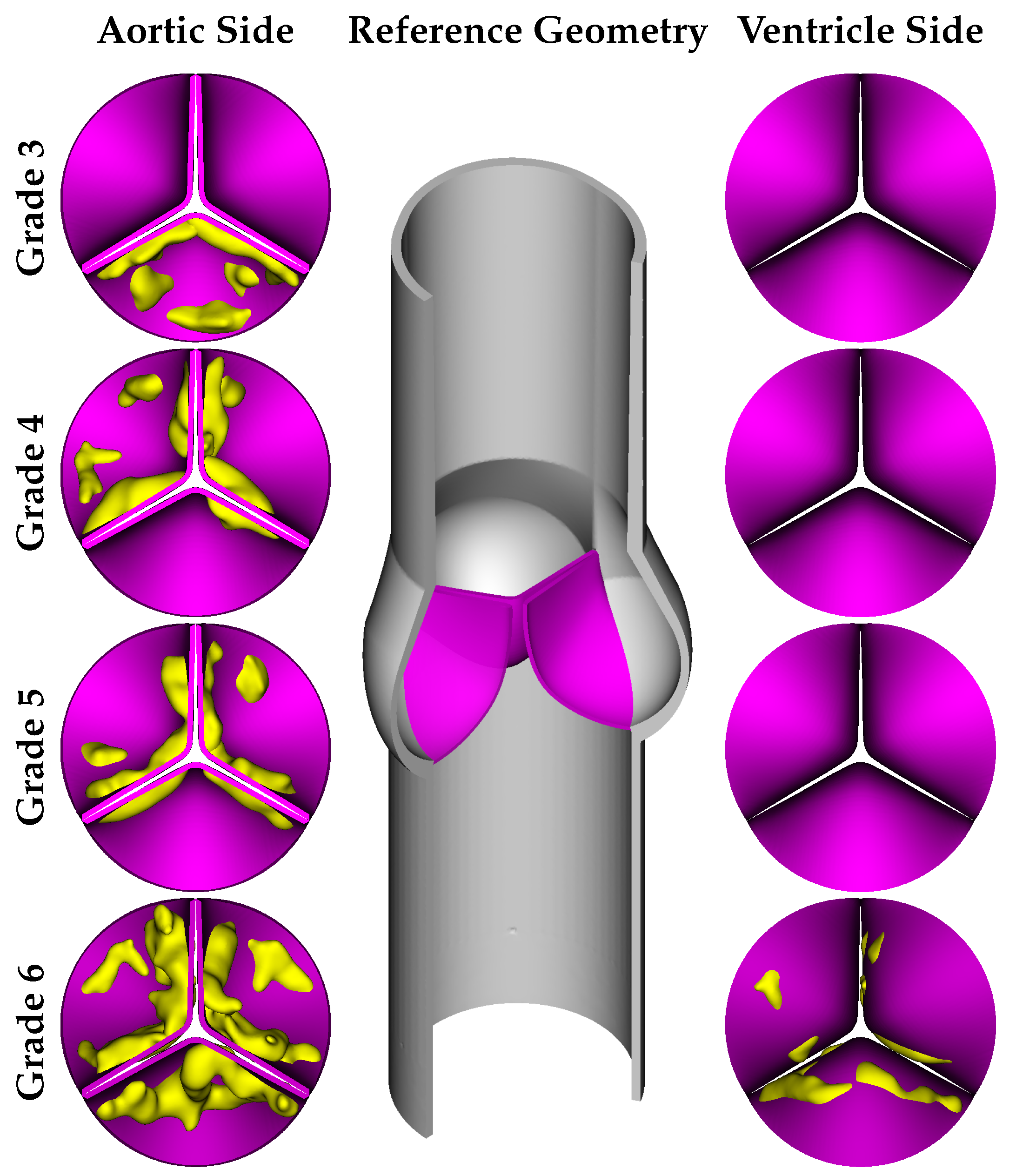
As Grade 2 calcification has a lower impact compared to the other grades, we did not include this grade in our simulations, and the calcified leaflet geometries were designed for Grades 3–6. As mentioned before, the main objective of our work was to analyze the influence of 3D calcification patterns on the hemodynamic behavior of aortic valve. For this goal, we adopted primary geometries of calcific deposits from the work of Lavon et al. [34] and combined them with the reference geometry of the native aortic valve. Model geometries were developed based on the various calcification patterns of several grades reported in the work of [33]. It should be noted that Grade 6 represents the most severe case, where the deposits are present on both the aortic and ventricular sides of the leaflets, as shown in Figure 1.

2.4. Numerical Schemes and Boundary Conditions

In our model, based on the immersed boundary finite element (IBFE) method, the fluid domain is discretized using a staggered block-structured fixed Cartesian grid. This grid is utilized to approximate the Eulerian variables, which include velocity, pressure, and force density, as described in Griffith and Luo [29]. Standard second-order accurate finite difference methods were employed to approximate the divergence, gradient, and Laplace operators [35]. For the convective term in the momentum equation, a version of the piecewise parabolic method (PPM) was used [36]. The Lagrangian variables corresponding to the immersed structure are represented by an unstructured finite element mesh. For the coupling between the Lagrangian and Eulerian variables, we used the four-point IB delta function kernel [37].

2.4.1. Fluid and Structure Domains Mesh

The fluid domain is a cubic box with dimensions of $0.116\mathrm{m}\times 0.116\mathrm{m}\times 0.116\mathrm{m}$ along the x, y, and z axes, respectively. We employed a $N\times N\times N$ Cartesian grid for the spatial discretization of the fluid region. The computational domain, which is based on Cartesian meshes with N selected as 78 and obtained through the mesh independence analysis presented in the following section, is shown in Figure 2. In order to improve the computational efficiency, a level of static mesh refinement was employed around the immersed structure, with a refinement ratio of four, resulting in a total grid size of approximately 4 million elements.

The reference aortic housing and valve structures were discretized using unstructured, first-order tetrahedral elements. Figure 3a–e displays the detailed view of solid regions and their meshes for the reference housing and for each grade of calcified aortic valve. In the IBFE method we adopted, the solution’s accuracy depends on the ratio between the Lagrangian element node spacing and the Eulerian grid spacing, referred to as the mesh factor or $M_{\mathrm{FAC}}$. Accordingly, we set the sizes of the structural mesh elements to achieve $M_{\mathrm{FAC}}$ values of approximately 1.0 near the wall and 0.5 around the valves [37]. The structural meshes consist of approximately 1.86 million elements for the native healthy aortic valve and 1.89, 1.88, 1.93, and 2.12 million elements for Grades 3 to 6, respectively.

2.4.2. Constraints and Boundary Conditions

To investigate the influence of both uniform and helical LVOT flow, we introduce an in-plane velocity profile to complement the through-plane waveform [38] at the inflow boundary. The amplitude of the in-plane waveform is set to half of the through-plane velocity during systole and zero during diastole. The through-plane velocity profile along the $+y$-direction and the in-plane velocity profile on the $xz$-plane, and the resulting Windkessel (WK) pressure profile at the outflow boundary, are given in Figure 4.

The velocity profile serving as the inflow boundary condition is imposed on the circular domain at the bottom wall of the computational box. The outlet pressure profile is dynamically determined using the three-element Windkessel (WK3) model, which is the most well-known Windkessel model with a proximal resistor ($R_p$) in series and a parallel combination of a distal resistor ($R_d$) and a capacitor (C). The three-element Windkessel model is governed by the following ordinary differential equation:

$$\left(1+\frac{R_p}{R_d}\right)Q\left(t\right)+C{R}_p\frac{dQ\left(t\right)}{dt}=\frac{P\left(t\right)}{R_d}+C\frac{dP\left(t\right)}{dt}$$

(9)

where $Q\left(t\right)$ is the flow rate, $P\left(t\right)$ is the pressure in $\mathrm{mmHg}$, $R_p$ is the characteristic impedance, C is the compliance, and $R_d$ is the peripheral resistance. The simulation initiates with an internal aortic pressure set at 70 $\mathrm{mmHg}$. The model parameters were selected as $R_p=0.033\mathrm{mmHg}·\mathrm{s}/\mathrm{mL}$, $R_d=0.79\mathrm{mmHg}·\mathrm{s}/\mathrm{mL}$, and $C=1.75\mathrm{mL}/\mathrm{mmHg}$ [38].

Equation (9) is discretized using a second-order backward finite difference scheme and divided into three parts as follows:

$$\mathit{LHS}=\frac{Q^n}{C}\left(1+\frac{R_p}{R_d}\right)+\frac{R_p}{\Delta t}\left(1.5Q^n-2Q^{n-1}+0.5Q^{n-2}\right)$$

(10)

$$\mathit{RHS}=\frac{1}{\Delta t}\left(-2P^{n-1}+0.5P^{n-2}\right)$$

(11)

$$\mathit{DNM}=\frac{1.5}{\Delta t}+\frac{1}{R_{d}C}$$

(12)

$$P^n=\frac{\mathit{LHS}-\mathit{RHS}}{\mathit{DNM}}$$

(13)

where n denotes the solution step and $P^n$ is the outflow pressure, which will be used as a Windkessel boundary condition in the following time step.

In cases involving calcification, the inlet flow rate is individually adjusted for each case using a unique factor with the goal of maintaining consistent aortic pressure above the valve while simulating increased LVOT pressure due to stenosis. Then, the flow rate factors for each calcification grade are defined as follows: $f_{\mathrm{No}-\mathrm{calcification}}=1$, $f_{G3}=0.75$, $f_{G4}=0.67$, $f_{G5}=0.67$, $f_{\mathrm{G}6}=0.48$.

2.4.3. Numerical Implementation

Since the blood flow in the aortic region is momentum-dominated, we used the Newtonian fluid model for blood, with dynamic viscosity and density values of $0.0035\mathrm{Pa}·\mathrm{s}$ and $1056\mathrm{kg}/{\mathrm{m}}^3$, respectively [39]. The simulations accounted for transient flow and initially covered two cardiac cycles, equivalent to $1.6\mathrm{s}$. We employed an explicit version of the Crank–Nicolson Adams–Bashforth scheme for time-stepping, with a time-step size of $\Delta t=1\times {10}^{-5}\mathrm{s}$, resulting in a maximum CFL number below 0.6 for all simulations. The linear system of equations given in Equations (1)–(4) for the flow velocity, pressure, and the location of the structure was solved via the flexible generalized minimal residual method (FGMRES) algorithm [40] with a projection method-based pre-conditioner [35]. The convergence of the solver was controlled by the relative residual tolerance, which was taken as ${10}^{-12}$ for all simulations, and this led to approximately 10 iterations for each time step and a maximum system residual below ${10}^{-6}$ for the continuity, velocity, and pressure of the system.

We conducted grid convergence studies to determine the consistency and accuracy of our numerical results. By generating four distinct mesh resolutions corresponding to an $N\times N\times N$ grid, with a one-level local refinement at a ratio of four, we compared the results for N values of 58, 68, 78, and 88. Our refinement approach ensured that the background Cartesian grid contained approximately one structural mesh node for each grid cell, leading to maximum element edge lengths for the finest grid at 0.5, 0.43, 0.37, and 0.33 mm for each respective N value. Considering the sensitivity of the IB method due to the coupling of Eulerian and Lagrangian variables, defining convergence for the numerical method is challenging [41]. Even minor alterations in the simulations, such as in grid spacing or time-step size, can significantly impact flow velocities and subsequent displacements. Our accuracy assessment involved comparing the average fluid velocity near peak systole across the aforementioned grid sizes.

Figure 5 represents this average fluid velocity, ranging from a time of $t=0.05\mathrm{s}$, to a final time of $t=0.2\mathrm{s}$. Across all tested grid resolutions, we observed consistent values. Though convergence is not explicit, and since the flow is transient, we expected that the average flow velocity would show convergence as t approached infinity. While our results are fairly well resolved for large-scale flow measurements, peak flow velocities in coarser cases exceed those in finer ones. These discrepancies in peak flow velocities stem from the numerical scheme employed to couple the Lagrangian and Eulerian variables in our IB method [42]. Such differences tend to diminish with grid refinement, as corroborated by our grid convergence observations. For greater accuracy, the mesh factor ($M_{\mathrm{FAC}}$) should be below one, meaning that the structural mesh must be refined correspondingly when the fluid grid is refined. However, due to the substantial computational costs of the $N=88$ case—which comprises roughly 6 million fluid mesh elements and 4.25 million structure mesh elements—we chose $N=78$ as the basis for our model.

We carried out our simulations at the National Center of High-Performance Computing of Turkey (UHeM) using the IBAMR 0.9.0 software framework [43]. The computing cluster was equipped with an InfiniBand^®-based network, AMD EPYC 7742 2.24 GHz CPUs, and 256 GB of RAM. Each typical simulation took approximately 240 h of wall clock time on one node with 128 cores, equivalent to roughly 30,000 CPU hours.

2.5. Comprehensive Quantification of Transvalvular Hemodynamic, Wall Shear Stress-Based Indices, and Helicity Descriptors

In this section, a comprehensive analysis is conducted to quantify various hemodynamic indices [11], WSS-based indices, and helicity descriptors pertinent to transvalvular flow. Traditional parameters such as the geometric orifice area, maximum jet velocity, kinetic energy, energy dissipation, and the magnitude of vorticity are studied. WSS-based indices such as time-averaged wall shear stress (TAWSS), oscillatory shear index (OSI), relative residence time (RRT), and transverse wall shear stress (transWSS) are also examined. In order to quantify the helical flow in the whole domain, helicity descriptors ($h_1$, $h_2$, …, $h_6$) are employed.

The geometric orifice area (GOA) at a time instant t is defined as the region on the aortic cross-sectional plane that is enclosed by the projected curves of the leaflet commissures, representing the opening through which blood flows on the plane of leaflet attachment.

Another key indicator of transvalvular hemodynamics is the peak jet velocity $\left(V_{\max }\right)$ passing the orifice area of the aorta. This metric serves as a basis for estimating the pressure differential across the valve, typically calculated via a simplified form of the Bernoulli equation. The $V_{\max }$ not only provides insights into flow dynamics but also has clinical implications for evaluating valve function and potential stenosis.

The next index for assessing transvalvular hemodynamics is the energy dissipation rate, which quantifies the real-time power depletion in the flow of blood. Expressed in Watts, and computationally derived as:

$${\dot{E}}_{\mathrm{diss}}\left(t\right)=\frac{d{E}_{\mathrm{diss}}}{dt}\left(t\right)={\int }_V\Phi dV$$

(14)

In this formula, $\Phi =\mathit{\tau }\otimes \nabla \mathbf{v}$ symbolizes a dissipation function, where $\mathit{\tau }$ denotes the viscous shear stress tensor. ${\dot{E}}_{\mathrm{diss}}\left(t\right)$ accounts for the power loss within the Valsalva sinus, extending into the ascending aorta, thereby providing insights into the energy loss associated with blood viscosity and the presence of aortic stenosis.

Another crucial hemodynamic variable is the kinetic energy of the blood flow, denoted by $E_{\mathrm{kin}}\left(t\right)$, which can be calculated using the formula:

$$E_{\mathrm{kin}}\left(t\right)=\frac{1}{2}{\rho }_f{\int }_V{\mathbf{v}}^{2}dV$$

(15)

where the integration is carried out over the volume of the aorta. $E_{\mathrm{kin}}\left(t\right)$ serves as an indicator of the blood flow’s mechanical energy, which interchanges with both the pressure and viscous dissipation components.

The final index for evaluating transvalvular hemodynamics is the mean magnitude of vorticity, assessed within the aortic volume. The vorticity magnitude can be calculated using the expression:

$${\Omega }_a\left(t\right)=\frac{1}{V}{\int }_V|\Omega |dV$$

(16)

which averages the vorticity over the aortic volume. This quantity is derived from $|\Omega |=\sqrt{w_x^2+w_y^2+w_z^2}$, which is the square root of the sum of the squares of the individual components of the vorticity vector $\Omega$, defined as the curl of the velocity vector $\mathbf{v}$.

The next critical category of hemodynamic metrics encompasses WSS-based indices. These parameters characterize the viscous forces acting upon the vascular wall by the surrounding fluid, described by the WSS. Mathematically, the magnitude of the WSS is represented as ${\mathit{\tau }}_w=\mathrm{WSS}=n_i·{\tau }_{ij}$, where $n_i$ is the surface normal vector and ${\tau }_{ij}$ denotes the viscous stress tensor.

The metrics of the TAWSS, OSI [44], RRT [45], and transWSS [46] were computed based on the subsequent formulas:

$$\begin{array}{cc}\hfill & \mathrm{TAWSS}=\frac{1}{T}{\int }_0^T{\mathit{\tau }}_{w}dt,\hfill \\ \hfill & \mathrm{OSI}=0.5\left(1-\frac{\left|{\int }_0^T{\mathit{\tau }}_{w}dt\right|}{{\int }_0^T\left|{\mathit{\tau }}_w\right|dt}\right),\hfill \\ \hfill & \mathrm{RRT}=\frac{1}{(1-2\times \mathrm{OSI})\times \mathrm{TAWSS}},\hfill \\ \hfill & \mathrm{transWSS}=\frac{1}{T}{\int }_0^T\left|{\mathit{\tau }}_w·\left(\mathbf{n}\times \frac{{\int }_0^T{\mathit{\tau }}_{w}dt}{\left|{\int }_0^T{\mathit{\tau }}_{w}dt\right|}\right)\right|dt.\hfill \end{array}$$

(17)

The helicity $H\left(t\right)$ of a fluid flow within a three-dimensional domain S is defined as follows [47]:

$$H\left(t\right)={\int }_S\mathbf{v}(\mathbf{x},t)·\mathbf{\omega }(\mathbf{x},t)dV={\int }_S{H}_k(\mathbf{x},t)dV$$

(18)

In this expression, $\mathbf{v}(\mathbf{x},t)$ and $\mathbf{\omega }(\mathbf{x},t)$ denote the velocity and vorticity vectors, respectively, while $H_k$ represents the helicity density. The sign of $H_k$ serves as an indicator of the rotational direction. Specifically, helical structures with a positive (negative) $H_k$ value are classified as right (left)-handed, with a clockwise (counter-clockwise) rotation when the thumb is oriented in the direction of the flow. The LVOT peak pressure gradient is predominantly used as a hemodynamic descriptor in patients with hypertrophic cardiomyopathy (HCM). However, in these patients, secondary alterations in aortic blood flow have not been extensively described. The presence of helical flow in the LVOT and the ascending aorta (AAO), as an indicator of flow derangement, can serve as a valuable marker. To assess the aortic bulk flow with respect to its helical characteristics and flow topology, we define six helicity-based descriptors as follows: [47]:

$$\begin{array}{ccc}{h}_1\hfill & =\frac{1}{T{W}_i{V}_i}{\int }_{T{W}_i}{\int }_{V_i}{H}_{k}dVdt,\hfill & h_2=\frac{1}{T{W}_i{V}_i}{\int }_{T{W}_i}{\int }_{V_i}\left|H_k\right|dVdt,\hfill \\ h_3\hfill & =\frac{h_1}{h_2},\hfill & h_4=\frac{|h_1|}{h_2},\hfill \\ h_5\hfill & =\frac{{\int }_{T{W}_i}{\int }_{V_{id}}dVdt}{{\int }_{T{W}_i}{\int }_{V_{im}}dVdt},\hfill & h_6=\frac{1/V_{id}{\int }_{T{W}_i}{\int }_{V_{id}}{H}_{k}dVdt}{1/V_{im}{\int }_{T{W}_i}{\int }_{V_{im}}{H}_{k}dVdt}.\hfill \end{array}$$

(19)

where $V_i$ denotes the volumetric domain under consideration, and $T{W}_i$ signifies the temporal window for integration. Additionally, $V_{id}$ is the volume corresponding to the predominant rotational direction, while $V_{im}$ is the volume associated with the less dominant rotational direction.

3. Results

Calcification of valve leaflets can adversely impact the aortic valve’s structural integrity, contributing to the diminished lifespan of bioprosthetic heart valves (BHV) and overall valve functionality. These calcified formations can induce shifts in transverse pressure gradients and shear forces, potentially leading to more severe medical complications. Therefore, understanding the hemodynamic changes around the aortic valve caused by localized calcification is crucial for addressing issues related to VHD. In the subsequent sub-sections, we conduct an analysis that spans multiple aspects, from the dynamic kinematics of the aortic valve to the evolving flow patterns across different grades of calcification. We also examine transvalvular hemodynamic indices and WSS-related parameters, and explore the complex vortex structures formed under two different LVOT flow conditions.

3.1. Valve Kinematics

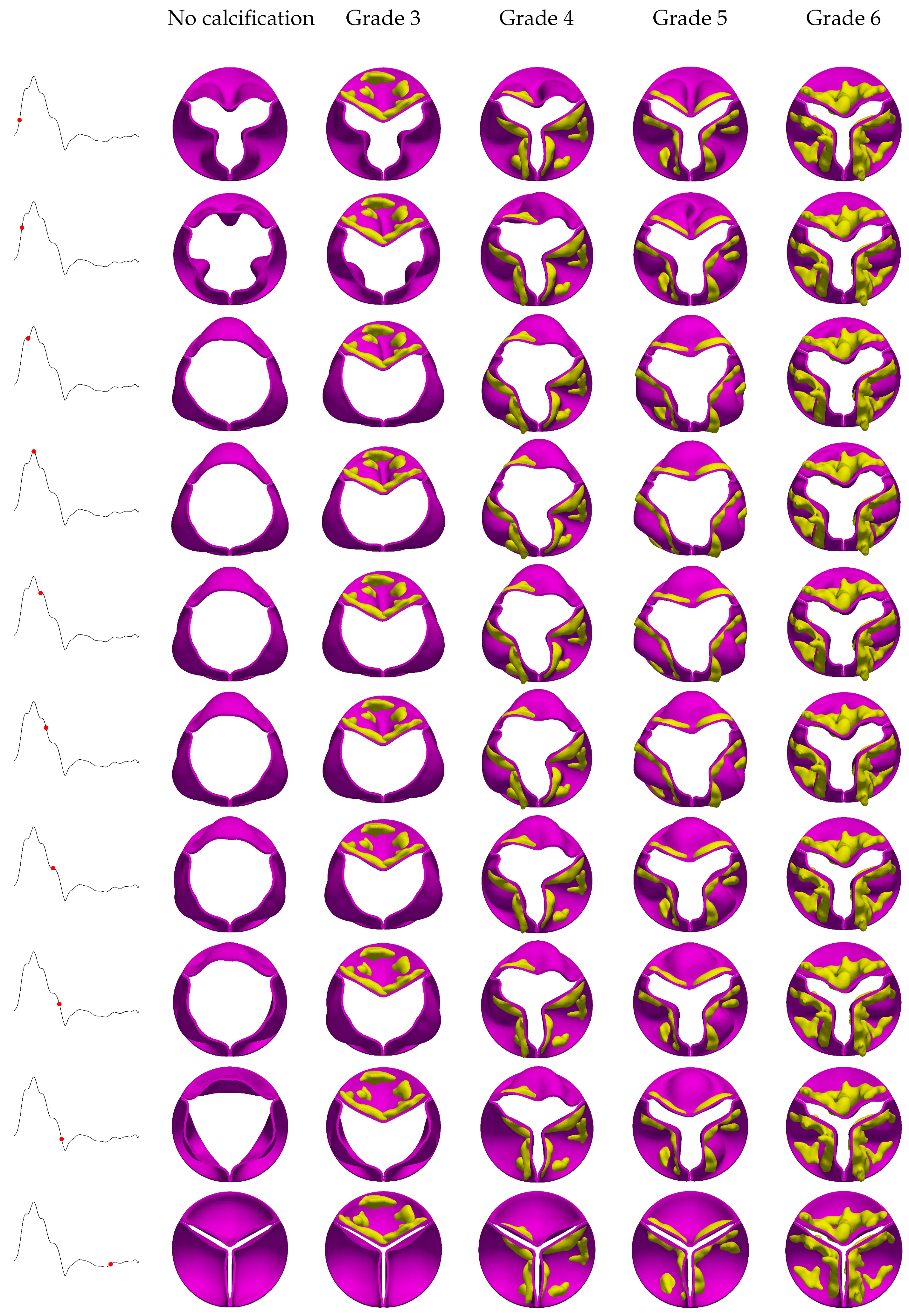
The stages of opening and closing for the aortic valve, observed across different calcification grades under both uniform and helical flow conditions, are illustrated in Figure 6 and Figure 7. One expected observation is that calcification disrupts the nearly symmetrical circular orifice observed in the absence of calcification. Figure 6 shows the evolution of valve kinematics over a cardiac cycle for various grades of aortic valve calcifications under uniform flow conditions. For instance, this asymmetrical behavior in Grade 3 shows itself as the restricted mobility of the heavily calcified leaflets forces the remaining leaflets to open excessively, a phenomenon readily apparent at peak systole. Conversely, in Grade 4, where two leaflets are significantly calcified, the third leaflet is forced into extreme opening, evidenced by its visibly distended shape. A comparison of calcific deposits in the coaptation zone and the belly region reveals more limited valve motion in the latter, with leaflets exhibiting convex shapes when deposits are localized to their coaptation areas. For Grades 5 and 6, where calcification is more uniformly distributed, symmetrical opening and closure were observed; however, increasing calcification severity correspondingly reduces the orifice area. As previously noted, LVOT flow can occasionally manifest as a helical pattern rather than a uniform one due to different anomalies such as HCM. Our simulations indicate that right-handed helical LVOT flow exerts a discernible influence on leaflet kinematics and morphology, as shown in Figure 7. Specifically, we observed a subtle counter-clockwise rotational tendency in the leaflets, along with occasional increases in their convex shaping.

These alterations are likely attributed to the helical flow’s additional radial components and their resultant interactions with the valve structure. Furthermore, the impact of helical flow on leaflet displacement and dynamics diminishes as the severity of calcification increases. The difference between leaflet behavior in helical and uniform inflow conditions is most pronounced in the absence of calcification and becomes progressively reduced as calcification reaches Grade 6.

3.2. Hemodynamic Flow Patterns in the Presence of Aortic Valve Calcification

To better understand the impact of localized calcification on valve leaflets, we analyzed 3D velocity streamlines at various intra-cardiac time points. Figure 8 shows these streamlines for the no-calcification case under uniform flow, and Figure 9 does the same for helical flow. In both cases, the simulations were conducted over two cardiac cycles, with the displayed results taken from the second cardiac cycle. In the no-calcification case of Figure 8, the aortic valve leaflets remain closed until the pressure in the left ventricle surpasses that in the aorta, prompting the valve to open approximately at $t=0.035\mathrm{s}$. Subsequently, the valve exhibits a fully circular orifice area where the maximum velocities occur right above the Valsalva sinus until the flow velocity reaches its peak during the systole phase. Up to this point, blood flows through the valve into the ascending aorta without noticeable resistance. Following peak systole, as the jet velocity diminishes, multiple vortices form due to flow separation at the leaflet tips and interact with the inner surface of ascending aorta. During early diastole, the aortic valve leaflets begin to close as the pressure in the left ventricle decreases below that in the aorta. This pressure difference initiates a deceleration of blood flow, and thus a loss of momentum and limited backflow towards the Valsalva sinus, aiding in the complete closure of the valve. Figure 8 shows that the spatial and temporal alignment of the Arantius nodules and coaptation lines of the no-calcification case are well coordinated and close in a timely manner.

As outlined in Section 2.3, Grade 3 represents a case where only one leaflet is affected by calcification. This condition leads to spatially asymmetric blood flow as the affected leaflet undergoes unstable displacement as expected. Unlike the symmetric flow observed in the no-calcification case, this asymmetry redirects the disturbed flow toward the inner wall of the ascending aorta. As a result, the flow circulates back toward the calcified leaflet, a phenomenon evident in vectorized flow plots of Figure 10 from the late systolic and velocity streamlines plots of the early diastolic phases in Figure 8. This circulating flow pattern contributes to the earlier closure of the calcified leaflet, as presented in the early diastole plots in Figure 8 and Figure 9. Furthermore, the magnitude of velocity in the ascending aorta reaches relatively higher values, likely attributable to the reduction in the valve orifice area. In contrast, the no-calcification case features a uniform jet flow through the orifice, whereas the presence of a constrained leaflet disrupts this flow, leading to a more chaotic jet stream.

In Grade 4 of the calcified aortic valve, two leaflets exhibit significant calcium deposits on their surfaces facing the ascending aorta. Increased calcifications, mostly located on the coaptation lines, generated greater valve opening resistance, leading to a reduced orifice area and elevated jet velocity. Unlike the uniform distribution observed in the no-calcification scenario, the jet in Grade 4 becomes narrower, and the magnitude of the velocity slightly increases in the centralized flow direction. As with Grade 3, the flow displays asymmetry, primarily due to the restricted mobility of the calcified leaflets. This results in a shift of the flow toward the third uncalcified leaflet during the flow acceleration phase. More chaotic flow patterns are evident during the deceleration phase, as shown in Figure 10, where asymmetric flow contributes to the earlier closure of the calcified leaflets, further increasing flow eccentricity with a highly chaotic turbulent behavior at the ascending aorta, as is evident in the early diastole plots in of Figure 8. This deviation in flow ultimately creates a strong vortex in the ascending aorta region, leading to increased energy dissipation.

In the Grade 5 scenario, an increase in calcification severity leads to a more powerful jet flow and unstable leaflet closure, as seen in Figure 8 and Figure 10. Due to the reduced orifice area, the jet’s width also narrows. In this grade, the calcification pattern is distributed almost symmetrically, resulting in a more balanced blood flow compared to Grade 4.

For the Grade 6 calcification scenario, the most severe among the studied cases, the highest jet flow velocity was observed as illustrated in Figure 8 and Figure 10, showing an increase of approximately 30% compared to Grade 3. This grade also has the longest and most sustained aortic jet, owing to the smallest $\mathrm{GOA}$, where the jet width is at its narrowest value. The deposits are relatively symmetrically distributed across all three leaflets, leading to nearly symmetrical leaflet opening and closure. However, this grade experiences the latest valve opening, with the smallest $\mathrm{GOA}$ generating the most intense vortex structures. The narrow jet flow results in more powerful backflow circulations toward the leaflets in the ascending aorta. Consequently, we observed that an increase in calcification severity leads to not only more disordered and turbulent flow patterns in the ascending aorta, but also more irregular leaflet dynamics, leading to shifted opening and closing.

Upon analyzing the temporal sequences of right-handed helical flow over a cardiac cycle, a discernible counter-clockwise rotational flow pattern manifests during both the acceleration and deceleration phases, as seen in Figure 9. In contrast to peak systole plots in a non-calcified context, the helical flow introduces a perturbation in the ascending aortic flow field, deviating from the nearly unidirectional behavior observed in uniform inflow scenarios; this results in a more turbulent flow regime with a higher $Re$ number (∼15,300). For the calcified cases during the deceleration phase, the aortic jet undergoes radial expansion, attributed to the inherent helical flow dynamics. This phenomenon engenders elevated levels of retrograde flow into the Valsalva sinus, as can be confirmed by visualizations at the early diastolic stage as shown in Figure 9 and Figure 10. The volume rendered velocity magnitude animations for each case are available in the Supplementary Materials section.

3.3. Transvalvular Hemodynamic Indices

The temporal variation of the GOA for both non-calcified and calcified aortic valves over a cardiac cycle taken from the second period of the simulations is illustrated in Figure 11. Due to the non-zero velocity profile during the diastole phase, which is a result of the chosen inflow profile, the valves remain slightly open before the onset of the second period. According to clinical data published by Thubrikar [48], the aortic valve area for a healthy valve falls within the range of 3.9 ± 1.2 ${\mathrm{cm}}^2$, where our results for the non-calcified case align with this range. It is evident that calcification significantly impacts leaflet opening, resulting in a substantial reduction in the orifice area. Our results indicate that increased calcification leads to delayed leaflet openings. In a healthy aortic valve, the leaflets typically open around 0.035 $\mathrm{s}$ during the first period. However, in diseased cases, the opening time exceeds this value, ranging between 0.038 and 0.47 $\mathrm{s}$ for Grades 3–6. This delay is primarily attributable to the increased resistance from the calcified leaflets. Additionally, an examination of the GOA curves for the calcified cases reveals that increasing calcification levels lead to more gradual leaflet closure, especially in the uniform flow case. A sudden spike in GOA was observed in the Grade 3 case under uniform flow due to the reversal of flow towards the uncalcified leaflets caused by flow deflection towards the wall by the calcified leaflet not occurring in the helical flow case. Similar to the opening phase, delays in leaflet closure were observed in calcified cases under a uniform flow pattern, resulting in severe regurgitation and insufficient blood flow to the ascending aorta. Upon examining the GOA curves under helical flow conditions, we observed a slight increase in GOA, and the delayed opening is evident, while all closings improved in these cases, referring to a slight improvement in regurgitation. However, the delay in closure is more uniform across all cases, occurring approximately at $t=1.125\mathrm{s}$.

In Figure 12, the maximum velocities of fluid flow through the orifice area are depicted for both uncalcified and calcified cases under uniform and helical inflow patterns. The velocity magnitudes of the jets were measured at a height of 0.068 $\mathrm{cm}$ from the inlet, indicating that the severity of calcification directly influences the jet velocities. Specifically, an increase in calcification severity leads to an elevated jet velocity, which can be attributed to the reduction in the orifice area required to maintain a constant flow rate. Interestingly, a pronounced spike in velocity was observed in Grade 3 during the valve’s closure phase. This phenomenon is due to a strong retrograde flow directed toward the valve, a result of the aortic valve’s asymmetric calcification pattern.

In the case of helical flow, the velocity trends largely mirror those observed under uniform flow conditions up to the point of peak systole. During the deceleration phase, however, a very slight increment in velocity was observed, on the order of 2–3%. This subtle difference is most noticeable when the velocity curves for uniform and helical flows are superimposed and could be attributed to the presence of additional radial velocity components. Moreover, the abrupt spike observed in uniform flow conditions is not present in the helical flow pattern. This absence may be due to the additional rotational velocity and the altered jet flow pattern in the helical case.

In Figure 13, the variations in kinetic energy in the Valsalva sinus and ascending aorta for different degrees of aortic calcification are illustrated under reduced flow conditions, which correspond to the role of severe aortic stenosis. In our computational simulations, kinetic energy was calculated in the volumes of the Valsalva sinus and the ascending aorta. We observed an unexpected decrease in kinetic energy as the severity of aortic calcification increased.

These findings are best understood within the context of our specific simulation parameters. Our model utilized a reduced flow rate to mimic the diminished cardiac output commonly associated with severe aortic stenosis. This reduction directly impacts kinetic energy, as $1/2\rho V^2$, leading to lower kinetic energy values, especially in areas distant from the stenotic orifice. Notably, the Valsalva sinus and ascending aorta are areas where kinetic energy could inherently be lower due to factors like the sinus’s expansion and the more disturbed flow in the ascending aorta. These regions may also experience further reductions in kinetic energy due to flow disturbances induced by calcification, except in Grade 3, which shows a sudden jump at the diastole phase due to severe asymmetry at a single leaflet in uniform flow. The same jump in Grade 3 is not visible in the case of helical flow, as seen in Figure 13.

Figure 14 and Figure 15 show the variations in the energy dissipation rate and the magnitude of vorticity in aortic valves with varying calcifications under uniform and helical flow conditions, respectively, over a cardiac cycle. The trends for both metrics are similar, suggesting that increased calcification in aortic valves contributes to the formation of more intense vortices and a corresponding rise in energy loss. For the non-calcified case, these metrics generally exhibit the lowest values, owing to the least resistance to blood flow. However, a slight increase in both the energy dissipation rate and vorticity magnitude was observed under helical flow conditions. Interestingly, the energy dissipation among the calcified leaflets does not follow a straightforward increase with the grade of calcification. Here, the influence of localized calcifications and their asymmetrical form with helical flow patterns becomes apparent. For example, Grade 3, which has only one calcified leaflet, shows a spike in both vorticity and energy dissipation during peak systole and backflow periods, likely due to intense fluttering of the free leaflets due to strong pattern asymmetry. Under uniform inflow, a second peak in these metrics is noticeable for all calcified cases during the valve-closure phase. However, this is not the case under helical flow for Grades 5 and 6, which show a more regular pattern. Grades 3 and 4, however, still exhibit a second peak, indicating that asymmetric calcification can have a negative impact on the vortical structures and consequent energy dissipation.

3.4. WSS-Based Hemodynamic Indices

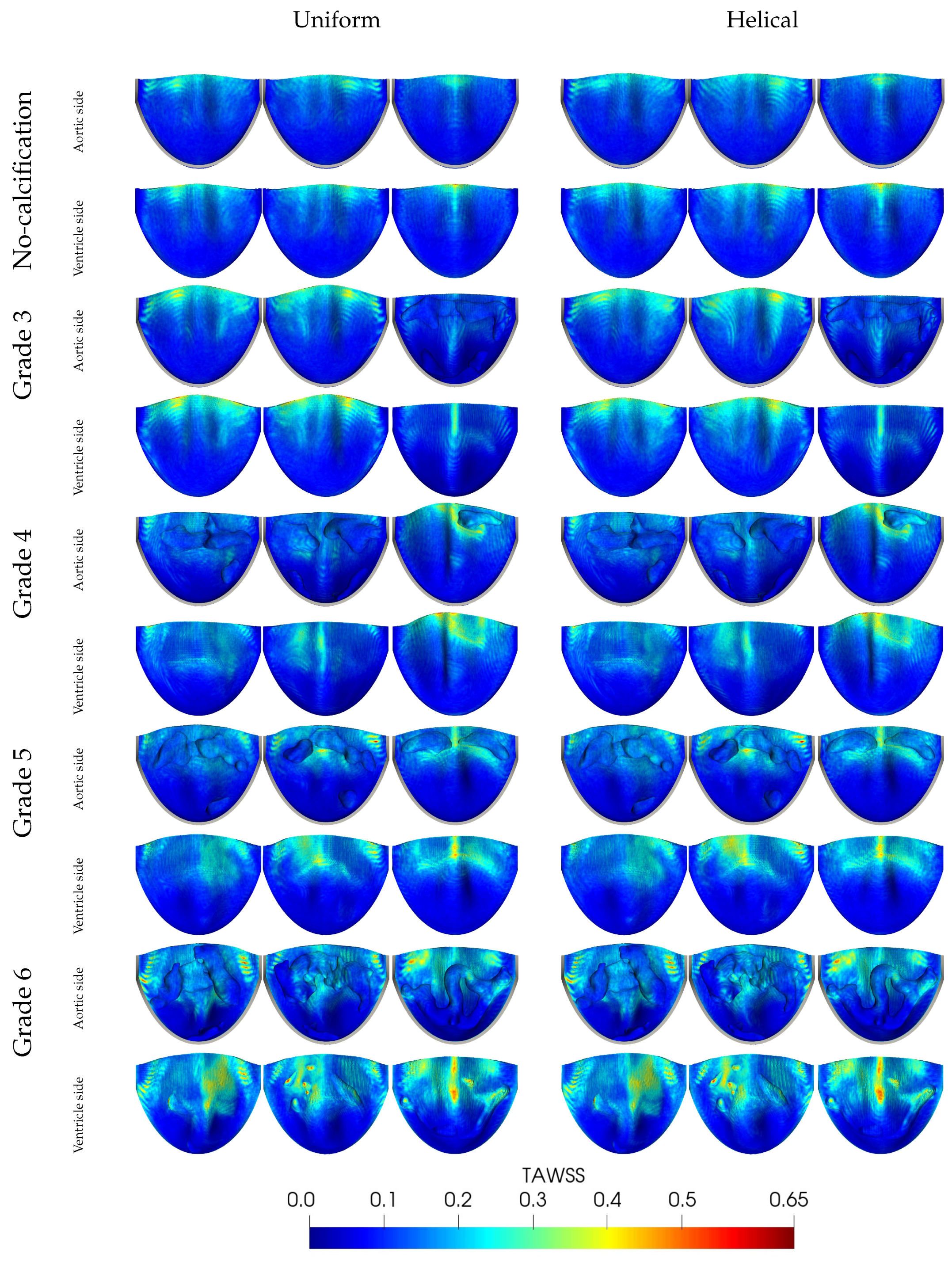
Since we use a Newtonian blood flow model, it is worth mentioning that non-Newtonian flow models appear at low strain rates; whereas aortic flow mostly generates mid- and high-strain rates where Newtonian blood flow treatment is considered to be a reasonable approximation. Therefore, we assume that the Newtonian flow model predicts WSS-based index values with an acceptable level of accuracy. TAWSS represents the cyclic average of the magnitudes of instantaneous WSS vectors. This index is presented in Figure 16 and shows significant variations with increasing calcification severity and different flow patterns. For instance, the tips of the leaflets are exposed to elevated TAWSS values due to greater fluttering, particularly when compared to the belly and root regions. As calcification becomes more severe, the increase in the TAWSS extends towards the belly region and mid-sections of leaflets. The presence of helical flow also slightly elevates TAWSS values and enriches the observed distribution patterns. The effect of calcification on the TAWSS also depends on the distribution, i.e., symmetry patterns of deposits. In Grades 3 and 4, where only one or two leaflets are calcified, the unoccupied leaflets demonstrate larger TAWSS values, possibly due to more intense contact and fluttering. Conversely, in Grades 5 and 6, all leaflets are calcified, resulting in a uniform TAWSS distribution across the leaflets.

We believe that one potential erroneous contribution to the asymmetric TAWSS contours in the no-calcification case resulted from placing the fluid domain’s staggered grid, with its 90-degree box shape, alongside the aortic valve and housing’s inherent 120-degree symmetry. This mismatch in grid symmetries led to asymmetry in the TAWSS for one leaflet, where normally, we would expect a similar distribution pattern with the other leaflets.

The OSI in Figure 17 serves as an indicator of the degree of reversing direction of the WSS within a cardiac cycle [49]. Thus, the OSI expresses the size of the changes in the direction and magnitude of the WSS. While the OSI reveals whether the WSS contains oscillatory components, it does not differentiate between unidirectional stress with varying magnitude and stress that changes in both magnitude and direction. A high OSI value, approaching 0.5, signifies an unsteady flow and is associated with a heightened risk of endothelial dysfunction and atherosclerosis in humans [45].

Generally, the OSI tends to inversely correlate with the TAWSS. In the case without calcification, the leaflets’ high and unrestricted flutter leads to OSI values close to 0.5, except in areas experiencing a high TAWSS at the tips. Calcification restricts leaflet movements, resulting in lower OSI values where the most heavily calcified Grade 6 leaflets exhibit the larger calcified areas with smaller OSI values. As expected, OSI values are generally lower on the ventricle side due to its exposure to more consistent unidirectional flow compared to the aortic side, which experiences more oscillatory flow due to vortex formation and retrograde flow. For helical flow, a slight but negligible change in OSI values was observed on both the aortic and ventricle sides. This suggests that the impact of helical flow on the OSI is minimal, at least within the scope of the conditions examined in this study.

The RRT, by definition, is an indicator of disturbed blood flow, marked by a low magnitude and high oscillatory WSS. In other words, it represents the time of residence the blood spent at the endothelium for the further formation of atherosclerosis localization. As shown in Figure 18, maximum RRT values are found at the roots of the leaflets, while minimum values occur at the leaflet edges due to the short blood residence time there. Increased calcification correlates with elevated RRT values, particularly at the roots of calcified leaflets. This suggests that blood stays longer behind calcification deposits. Notably, in Grade 5, where calcification is aligned along the coaptation line, elevated RRT values were observed in the belly region on both the aortic and ventricular sides. This can be attributed to the limited motion of leaflet tips during acceleration and deceleration, resulting in a concave leaflet shape that tends to keep blood for extended periods. Generally, RRT values are lower on the ventricular side due to continuously streaming blood flow as expected. Comparisons between uniform and helical flow reveal that RRT values decrease in helical flow scenarios, likely due to enhanced blood washout in the Valsalva sinus region. Moreover, the OSI and the RRT, which are both derived from the wall shear stresses, were used as further indicators of the increased risk of thrombus formation. Specifically, the regions with low OSI and high RRT values are good candidates for this.

The last WSS-based hemodynamic index analyzed in this study is transWSS, which measures the average of the WSS components perpendicular to the temporal mean WSS vector over a cardiac cycle. A low transWSS value indicates that the flow remains predominantly parallel to an axis along the main flow direction throughout the cardiac cycle. In contrast, a high transWSS suggests significant fluctuations in the radial flow direction. As displayed in Figure 19, calcification generally leads to increased transWSS values near the leaflet tips and belly region. Enhanced transWSS patterns were notably seen along the coaptation line due to the high flutter in this valve region. Higher transWSS values were observed in both Grade 3, with two leaflets without calcification, and Grade 4, featuring one with slight calcification. A broader transWSS distribution extending to the belly region was observed in Grade 6, likely due to reduced flutter at the leaflets’ tips and decoupled leaflet interactions with the ventricular blood flow. The results show that helical flow also contributes to elevated transWSS values on both ventricle and aortic sides. This is expected as transWSS primarily evaluates stress variations in directions perpendicular to the main flow. Thus, increases in transWSS arise from greater lateral load components, particularly in cases with generally asymmetric calcification patterns that induce temporally and spatially unstable fluctuations.

3.5. Quantification of the Helicity

The results so far show that helicity, in general, is considered to have favorable physiological effects as it promotes efficient transportation of blood, reduces flow disruptions, and helps prevent the accumulation of blood stasis behind the leaflets and aortic sinuses. In Section 2.5, six helicity-based bulk flow descriptors are presented. The helicity descriptors for both uncalcified and calcified aortic valve scenarios, under both uniform and helical flow conditions, are summarized in

Table 2. Helicity descriptors for the calcification grades under uniform and helical inflow.

Helicity Descriptors	Uniform					Helical
	No Calcification	Grade 3	Grade 4	Grade 5	Grade 6	No Calcification	Grade 3	Grade 4	Grade 5	Grade 6
$h_1$	−0.204	0.352	−1.381	0.989	1.206	14.550	9.368	3.816	6.803	5.372
$h_2$	0.418	1.521	1.606	1.866	1.398	71.374	82.921	86.552	75.592	95.855
$h_3$	−0.488	0.231	−0.860	0.530	0.863	0.204	0.113	0.044	0.090	0.056
$h_4$	0.488	0.231	0.860	0.530	0.863	0.204	0.113	0.044	0.090	0.056
$h_5$	0.996	1.024	0.983	1.025	1.013	1.261	1.101	1.051	1.039	0.955
$h_6$	−0.994	−1.000	−0.977	−1.067	−1.021	−0.883	−0.928	−0.877	−0.934	−1.025

. These values, obtained from the Valsalva sinus and ascending aorta, were integrated over the second period. The helicity-based descriptors offer valuable insights into the intricate flow changes and helical characteristics of flow topology induced by aortic valve calcifications.

The first descriptor, $h_1$, gives the time-averaged helicity, normalized by $V_i$, serving as an integrated measure of helical flow that takes into account the changes in the sign of $H_k$. For uniform flow, the $h_1$ descriptor suggests that the severity of calcification directly correlates with an increase in helical flow. A zero $h_1$ value signifies reflectional symmetry in the flow. While a $h_1$ value of $-0.204$ for the no-calcification case indicates a minor left-handed helical flow, this case is the closest to having reflectional symmetry among all the considered scenarios. Interestingly, the Grade 4 case has a left-handed flow trend, whereas Grades 3, 5, and 6 exhibit right-handed helical flows. In the context of helical inflow, $h_1$ values see a dramatic rise due to the inherent characteristics of the flow patterns. However, as the calcification grade increases, $h_1$ values tend to decrease. This suggests that higher grades of calcification disturb the flow, thereby reducing its helicity. Specifically, the lowest $h_1$ value for Grade 4 indicates a shift toward a left-handed helical flow. The second descriptor, $h_2$, shows the integration of the absolute value of $H_k$, reflecting the total helical flow in the domain without considering its direction. The $h_2$ values rise along with the severity of calcification, implying that helical flow structures are intensified due to the increased stiffness of the valve leaflets and asymmetric flow conditions. Notably, the elevated $h_2$ values for Grades 3 and 4, when compared to Grade 5, highlight the impact of localized calcification on one or two leaflets. The third descriptor, $h_3$, ranges from −1 to 1 and indicates the presence of left-handed (negative) or right-handed (positive) helical structures within the domain. The descriptor $h_4$ emphasizes the balance between opposing rotational structures and disregards the major rotation direction. The descriptors $h_3$ and $h_4$ tend toward zero as the calcification grade increases, suggesting that the natural helical flows set by inflow conditions become increasingly disrupted, resulting in less coherent vortices. The fifth descriptor, $h_5$, computes the proportion between the volumes of $V_{id}$ and $V_{im}$, while the sixth, $h_6$, calculates the ratio of $H_k$ values across the same volumes. Values of $h_5$ exceeding one for the uncalcified and Grades 3–5 cases suggest a higher volume occupied by the dominant rotational direction. Conversely, lower $h_6$ values for these grades indicate a lower rotational intensity. In contrast, Grade 6 shows a higher volume occupied by the minor rotational direction, as indicated by $h_5$, while $h_6$ reveals higher intensity in the dominant rotational direction. Overall, these findings strongly indicate that each case of aortic valve calcification generates a distinct helical flow tendency, which is significantly amplified by the presence of the helical inflow pattern, with likely implications for the progression of cardiovascular diseases.

3.6. Vortex Dynamics

To better understand the dynamics of the flow field and identify coherent structures during valve opening, we employed the Q-criterion, which essentially identifies vortices in areas where the vorticity magnitude exceeds the magnitude of the strain rate. Figure 20 illustrates the iso-surfaces of the instantaneous Q-criterion, which is used to visualize the instantaneous vortical structures at $t_1=0.05\mathrm{s}$, $t_2=0.06\mathrm{s}$, and $t_3=0.125\mathrm{s}$ during the systole phase. As the valve begins to open from a fully closed position, distinct vortex rings develop around the initial jet. Just after the valve opens, a three-lobed starting vortex emerges from the leaflet tips. As the flow accelerates, the vortex patterns become more intricate. At $t_1=0.05\mathrm{s}$, the primary vortex ring at the front of the jet and the subsequent second ring are evident in the no-calcification case under uniform inflow. As the jet progresses, additional vortex rings form due to the roll-up of the unstable shear layer surrounding the jet. The third vortex ring in the no-calcification case is visible behind the second one at $t_2=0.06\mathrm{s}$. These rings occasionally connect loosely, forming an approximate closed loop. Moreover, these rings are not entirely distinct; instead, they are connected by vortex filaments where the distances between the rings appear to grow gradually, a result of the increasing flow speed. As the flow rate climbs and peaks at $t_3=0.125\mathrm{s}$, vortex rings cease to form, and instead, vortices rapidly disintegrate into longitudinal filaments that lack clear structure. The presence of calcification impacts the formation of vortical structures, causing the normally circular vortex rings in a healthy valve to become asymmetric and tortuous in all calcified cases. With increasing calcification grades, the number of small-scale vortices among the vortex rings rises, and their interference with the rings makes the latter challenging to discern. Both the distance between the vortex rings and their width decrease, which can be attributed to the reduced orifice area and constrained leaflet dynamics of the valve. It should be noted that these snapshots are taken from the first period of the inlet profile. This is because the valves are initially closed at the start of the simulation, making vortex shedding more evident. In contrast, at the beginning of the second period, the valves are slightly open due to the specific diastole velocity used, causing unclear vortex formations from the CFD standpoint. Furthermore, results show that when calcification grades increase, the formation of the vortices delays and decreases in size, and the formation of small-size vortices drastically increases and fills the gaps due to the asymmetric and constrained dynamics of the valve leaflets. The increase in jet velocity and asymmetric leaflet dynamics at time $t_3=0.125\mathrm{s}$ cause a drastic increase in small-scale vertices in the ascending aorta during the systolic phase.

4. Discussion

We studied the hemodynamic implications of localized aortic valve calcifications in comparison to a healthy valve, using both uniform and helical blood inflow with realistic boundary conditions. To further understand the effects of helical LVOT flow, we incorporated an in-plane velocity profile alongside the through-plane waveform at the inflow boundary. For the outlet boundary condition on the aortic side, we employed the traditional three-element Windkessel model. Although this model does not capture pulse wave propagation, it offers a straightforward approach to ensuring an accurate physiological pressure at the outlet. To assess the impact of calcification on aortic valve performance, we utilized FSI simulations, through which we examined a range of hemodynamic parameters encompassing transvalvular flow fields, indices, WSS-based metrics such as TAWSS, OSI, RRT, and transWSS, and analyzed the intricacies of helical flow by quantifying helicity using various descriptors.

In localized calcifications, we observed restricted leaflet movement and a decreased orifice area, fundamentally altering the valve’s hemodynamics. Leaflet stiffening restricts the valve’s opening, compromising blood transport efficiency and subsequently imposing additional stress on the left ventricle, aligning with clinical findings. The constricted valve opening in calcified valves leads to a flow jet at the orifice, which, in turn, promotes circulatory flow and intensifies turbulence within the aortic sinuses. The aortic orifice area typically ranges from 3.9 ± 1.2 ${\mathrm{cm}}^2$ for healthy conditions to 1.0–1.5 ${\mathrm{cm}}^2$, in cases of moderate stenosis, and our findings confirm these metrics, consistent with clinical observations detailed in [4]. These different levels of calcification are notably correlated with significant disparities in resulting flow patterns, the magnitude of vorticities, and, consequently, the forces exerted on the aorta walls and valve leaflets. The asymmetrical formation of calcification deposits on one or two leaflets leads to additional stress on the remaining non-calcified leaflets. Unlike previous studies [11,50,51] that focused on uniformly calcified leaflets, our findings indicate that localized calcification directs the flow towards the ascending aorta’s wall, and the study by [52] suggests this redirection has the potential to cause harm to the wall. Some research suggests this redirection has the potential to cause harm to the wall [52]. This redirection results in periodic elevated WSS, which may accelerate endothelial erosion and nitric oxide (NO) release over time [53]. Increasing calcification severity also leads to the formation of stronger vortices and, consequently, greater energy dissipation rates. These findings align with prior works, specifically, the studies by Halevi et al. [4] and Gilmanov et al. [11], but offer a more in-depth perspective by examining the localization of calcification.

Alterations in blood flow directly influence the distribution of WSS on the leaflets, a factor significant for calcification progression [54]. Our simulations demonstrate that, compared to healthy scenario, calcified leaflets undergo markedly elevated WSS. Our study revealed a marked impact on WSS-based indices, with a higher TAWSS being associated with more advanced calcification grades, suggesting an increased risk of endothelial damage. The leaflet’s base region, proximate to the aortic root, maintains a fairly stable and low TAWSS irrespective of calcification levels. Conversely, the calcified leaflet’s tip undergoes prolonged exposure to elevated WSS and demonstrates a significant susceptibility to calcification grades. As calcification intensifies, the leaflets encounter increasingly spatially complex shear stresses, amplifying the TAWSS disparity between tip and base regions. In scenarios of pronounced calcification, the leaflet tips are subjected to exceptionally high shear stresses. As expected, varying calcification patterns instigate distinct flow behaviors and vorticity intensities, subsequently affecting shear stress magnitudes and distributions, especially adjacent to the leaflets—a phenomenon affirmed by our results. The aortic side experiences significantly reduced WSS in contrast to the ventricular side, with the difference amplifying as calcification escalates. In alignment with prior studies highlighting the aortic side (or fibrosa) to be more susceptible to calcification than the ventricle side (or ventricularis) [4,10,55], our results support this finding, substantiating that diminished TAWSS levels on the aortic side foster calcific particle deposition on the fibrosa layer. Thrombosis tends to form in regions with low flow or stasis, where shear stresses are reduced [56,57,58]. Given these insights, it is beneficial to have a high probability of elevated shear stress close to the leaflet. Conversely, a decreased probability of such stress is undesirable, as regions with diminished shear stress have a greater risk of thrombus formation [58]. OSI values are generally lower on the ventricle side compared to the aortic side, which experiences more oscillatory flow due to vortex formation and retrograde flow. A slight but negligible increase in OSI values is observed for helical flow. RRT values are lower on the ventricular side due to transit blood flow, and similarly, helical flow RRT values decrease due to enhanced blood washout in the Valsalva sinus region. Simultaneously observing higher values of RRT in the attachment line on the ventricle side of the healthy valve, which is consistent with the findings presented by Sarbandi et al. [10], we also noted an escalation of RRT values in the vicinity of the aortic root with increasing calcification; this is crucial as certain clinical data highlight the potential for thrombus formation within the attachment region of transcatheter aortic valves [59]. Calcification notably elevates transWSS values, especially in leaflet tip regions, with distinct patterns and variations arising across different calcification grades and regions. Enhanced transWSS is prominently observed along the coaptation line and is influenced by both leaflet flutter and helical flow. Notably, asymmetrical calcification patterns cause unstable fluctuations, impacting stress variations and lateral load components.

We found nuanced shifts in helical flow characteristics with increasing calcification severity; specifically, higher grades of calcification suppress the helicity while increasing its intensity in the ascending aorta. Aortic helical flow, commonly seen in healthy individuals, stems from the cardiovascular system’s innate ability to optimize fluid transport processes [60]. Localized calcification disrupts the naturally formed helicity in the flow field of the aortic domain, potentially affecting blood transport efficiency and contributing to further cardiovascular disease progression. A deeper exploration of the helical flow patterns is undertaken through helicity descriptors. Our results indicate that helicity has favorable physiological implications, as it promotes efficient blood transportation, minimizes flow disruptions, and reduces the accumulation of blood stasis behind the leaflets and aortic sinuses.

Finally, investigating the vortical structure formations, distinct vortex rings become evident as the valve opens, with their complexity growing as flow increases. We found that calcification noticeably impacts these vortex formations. In healthy valves, symmetrical vortex rings are evident, while in the presence of calcification, these rings become distorted. The increasing presence of small vortices with rising calcification grades further obscures these vortex structures. This is intensified at $t=0.125\mathrm{s}$, which is attributed to a heightened jet velocity and altered leaflet dynamics, resulting in a significant increase in smaller vortices in the ascending aorta during systole.

Our model has some limitations, such as the assumption of uniform deposit volumes and the absence of in vivo validation. Future research should aim for more realistic fluid–structure interaction (FSI) models with various calcium deposit stiffnesses, patient-specific calcification patterns with different aortic root diameters, and flow conditions. Further validations for both the long-term clinical impact of altered hemodynamics and in vivo results are suggested.