

Bisection Constraint Method for Multiple-Loading Conditions in Structural Topology Optimization

Abstract
:1. Introduction
1.1. Topology Optimization (TO)
1.2. Topology Optimization Considering Multiple-Loading Conditions
2. Topology Optimization under Single- and Multiple-Loading Conditions
2.1. SIMP Approach
2.2. Single-Loading Condition
2.3. Multiple-Loading Conditions
2.4. The Min–Max Compliance Problem in TO Considering Multiple-Loading Conditions
3. Bisection Constraint Method for Topology Optimization Considering Multiple-Loading Conditions
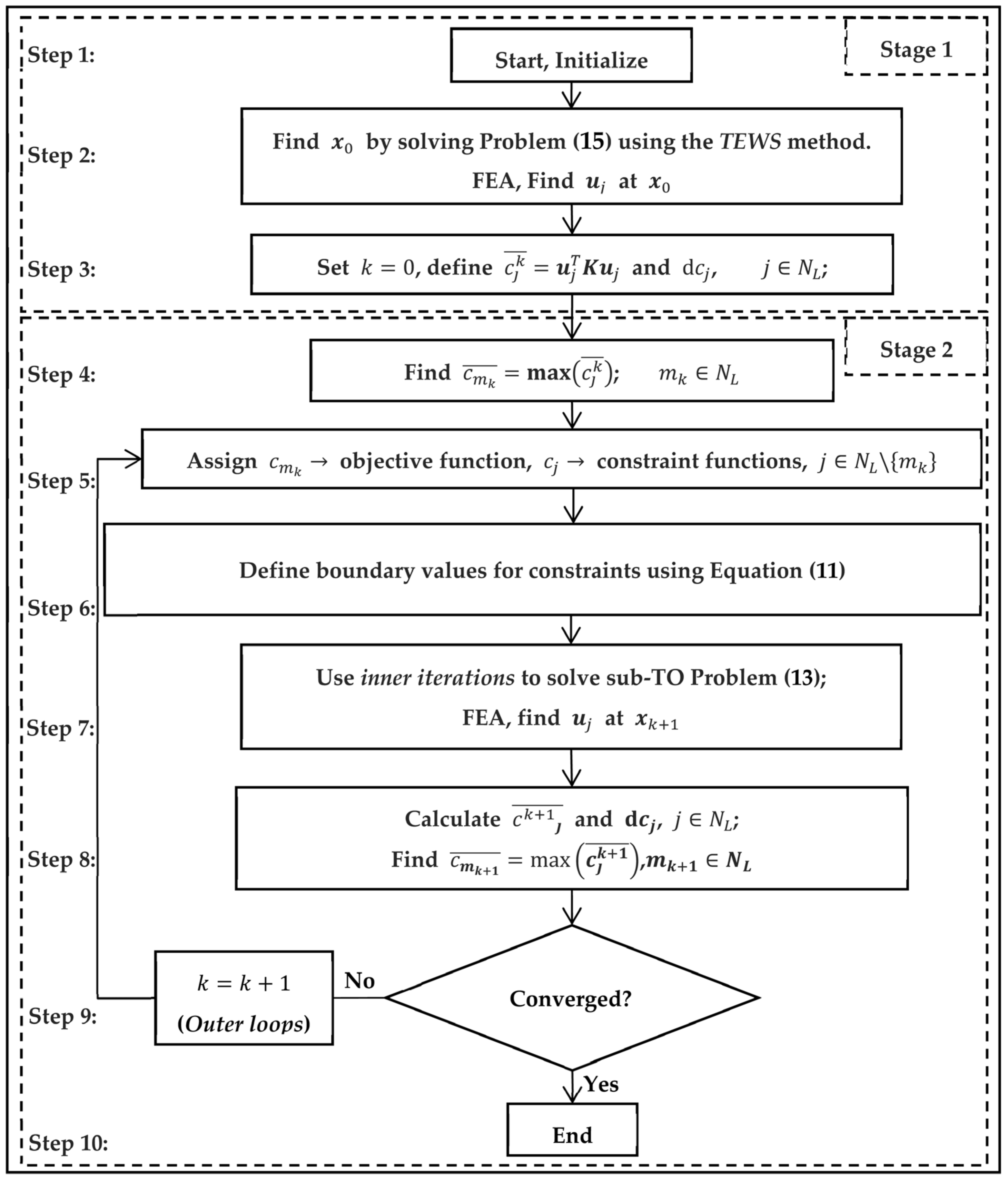
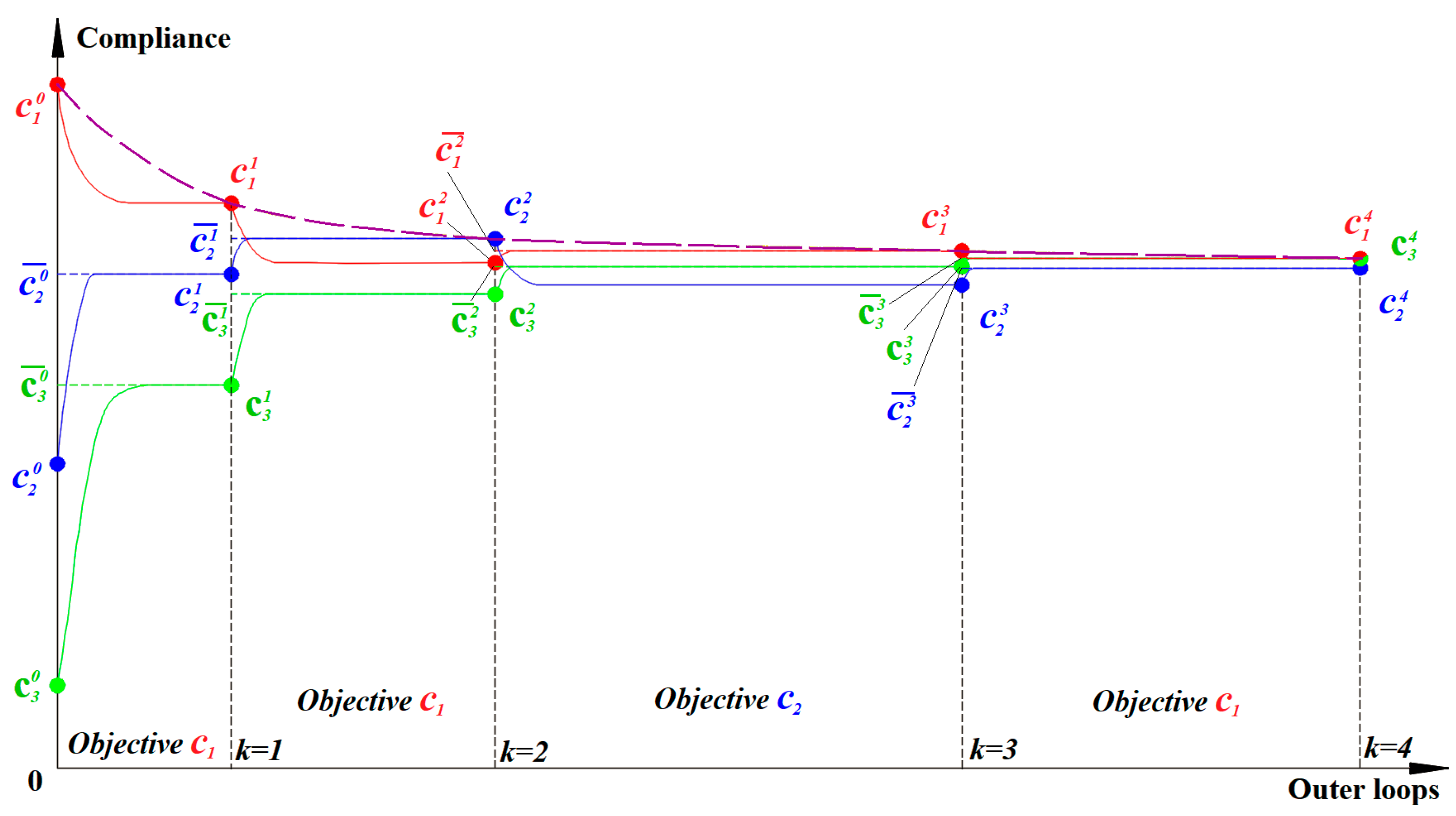
3.1. The Bisection Constraint Method
3.2. Starting Point
3.3. Termination Criterion
4. Application of the Proposed Method
4.1. Case Study 1
4.2. Case Study 2
5. Comparison of the Proposed Method with the Weighted Sum Methods
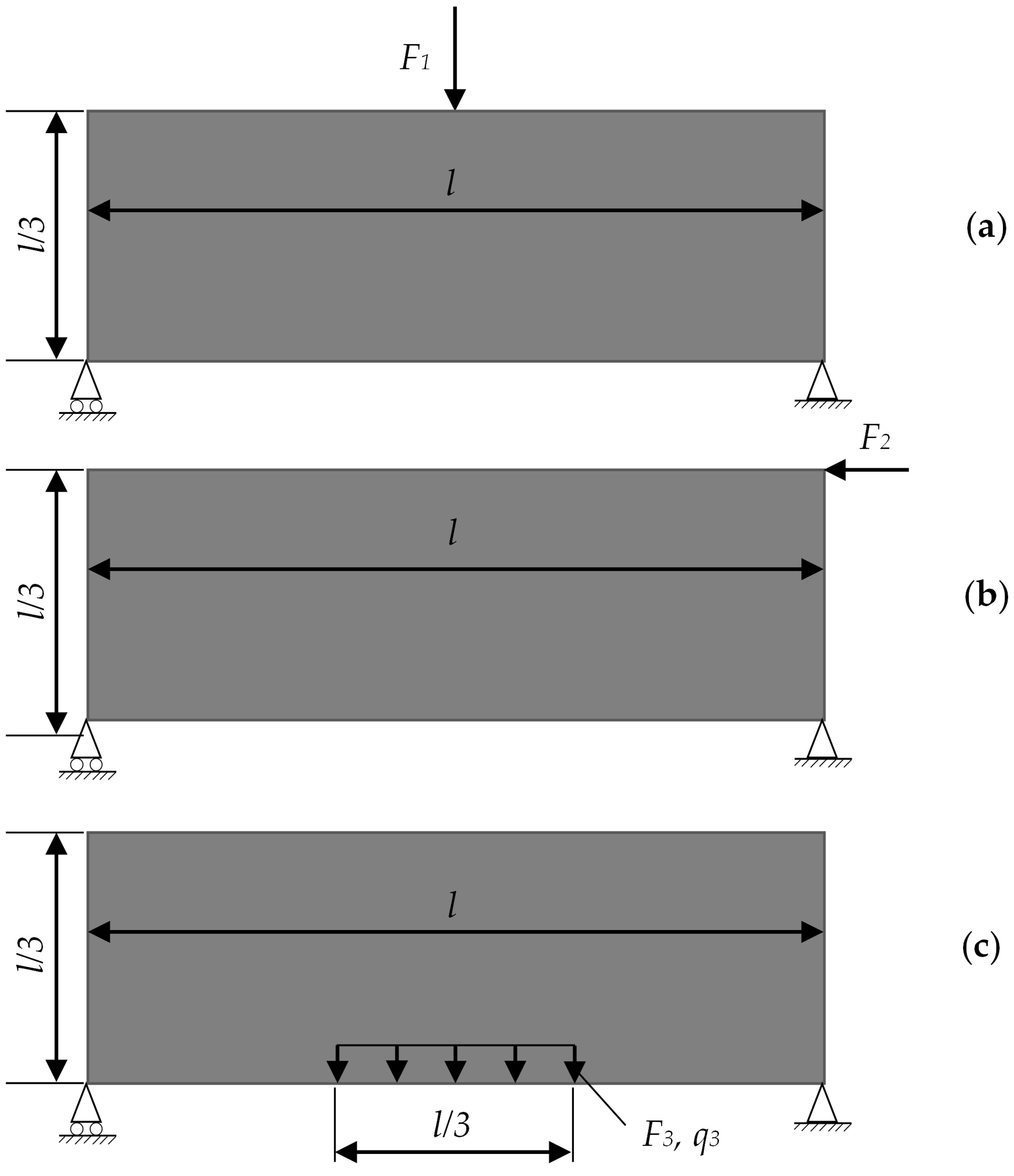
5.1. Loads Are Borne by the Entire Structure
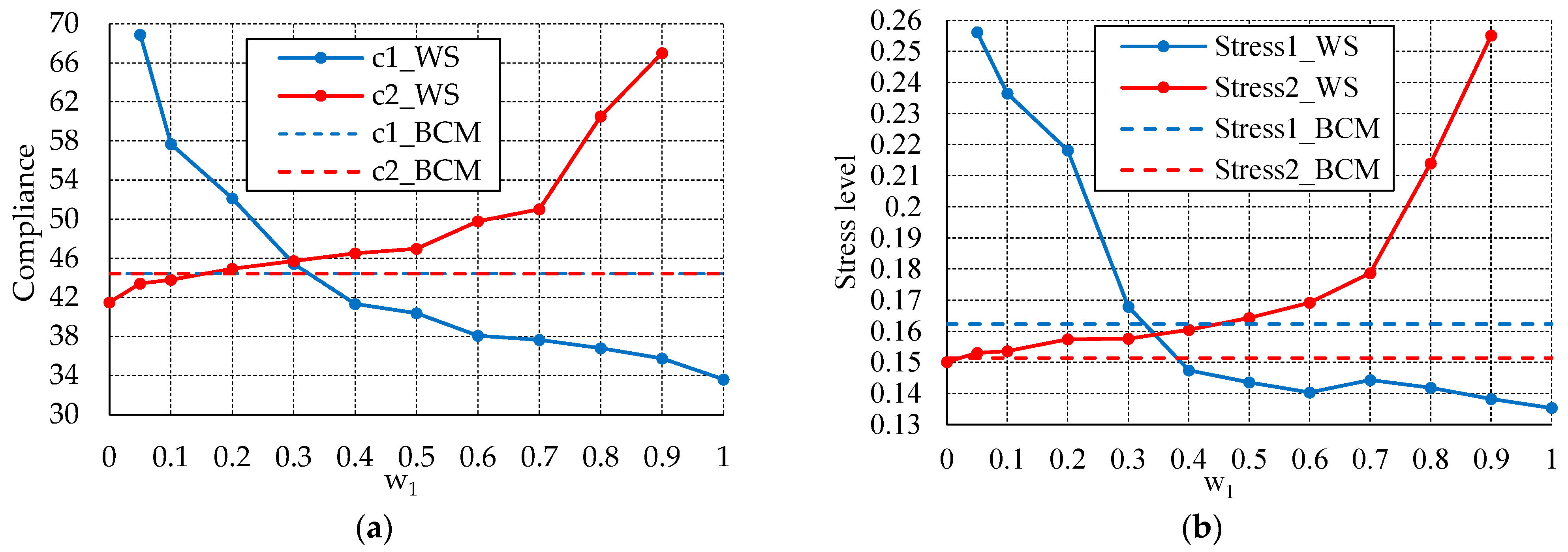
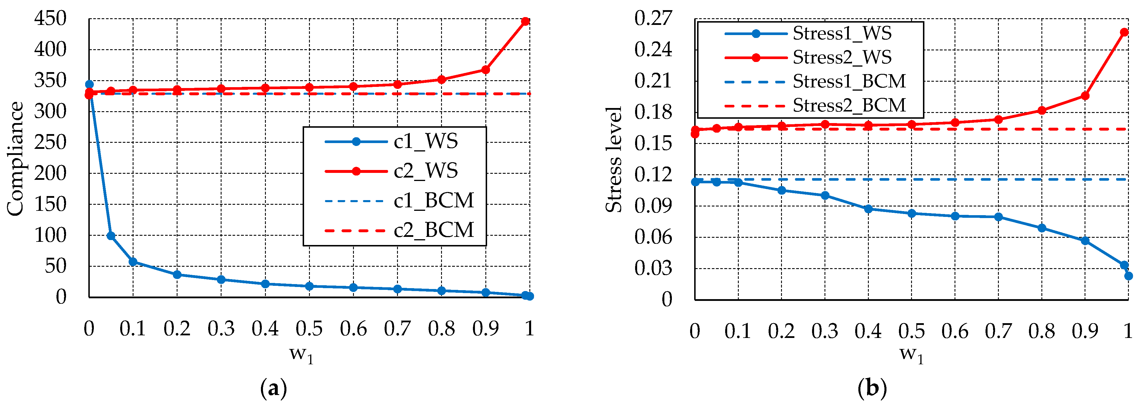
5.1.1. Problem 1
- (a)
- When and
- (b)
- When and
- (c)
- When and
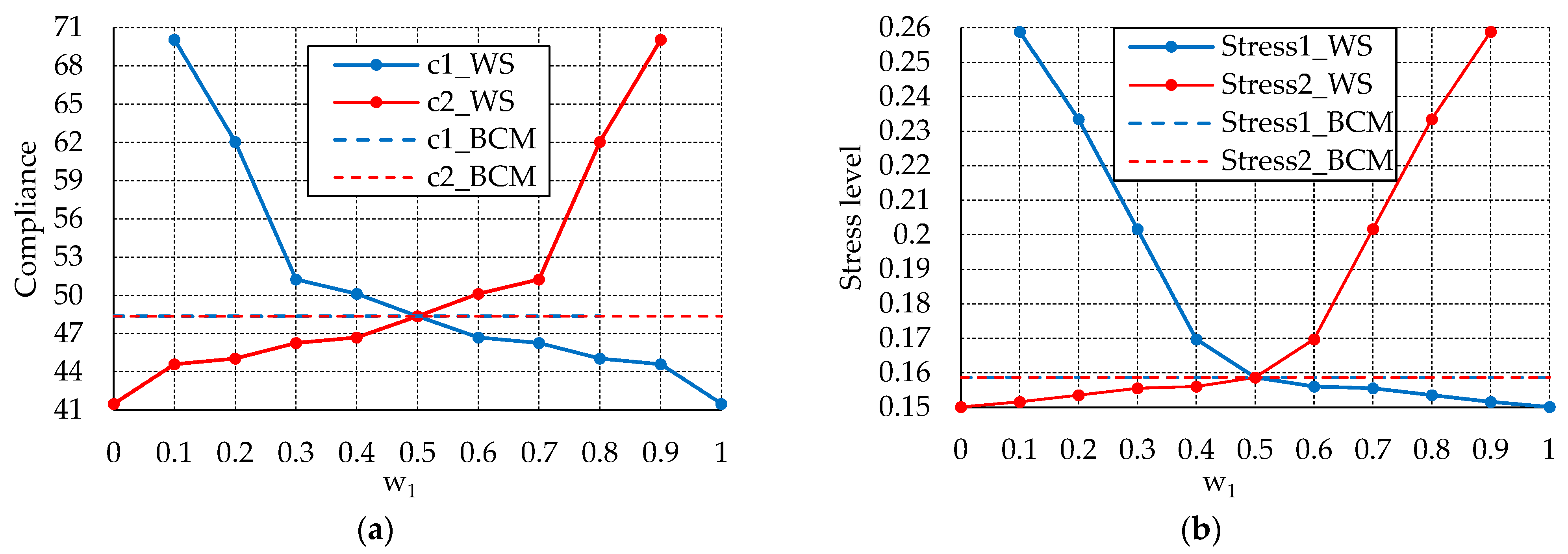
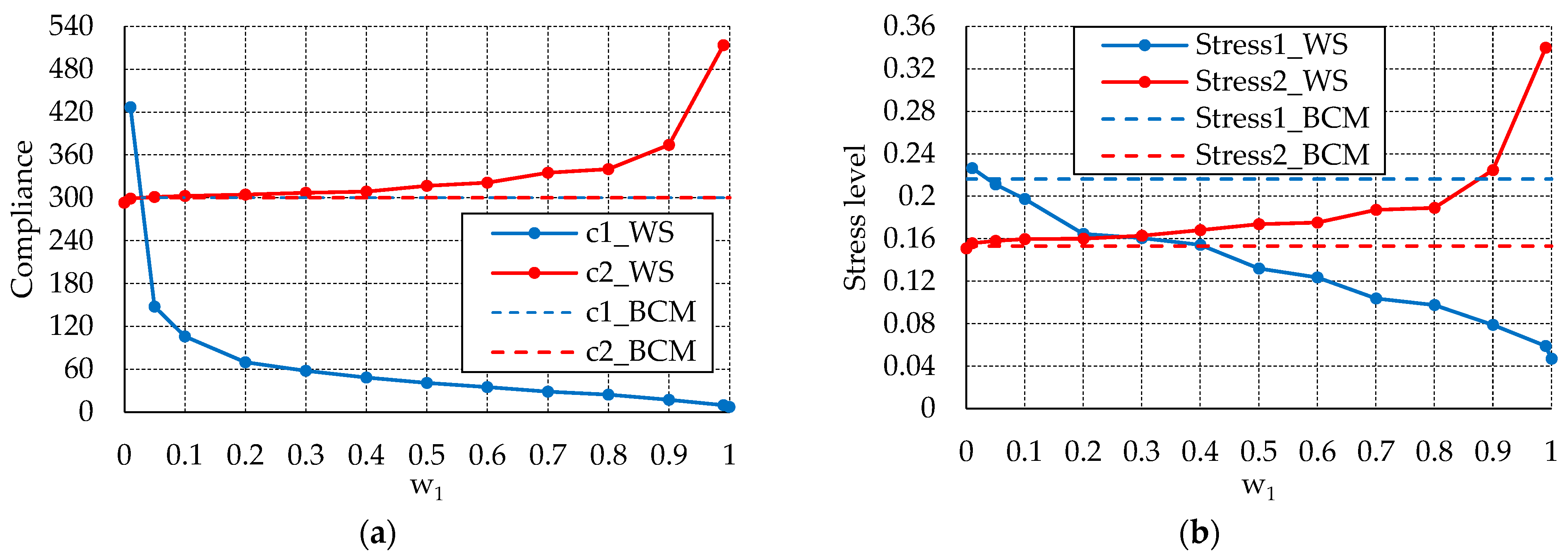
5.1.2. Problem 2
- (a)
- When and
- (b)
- When and
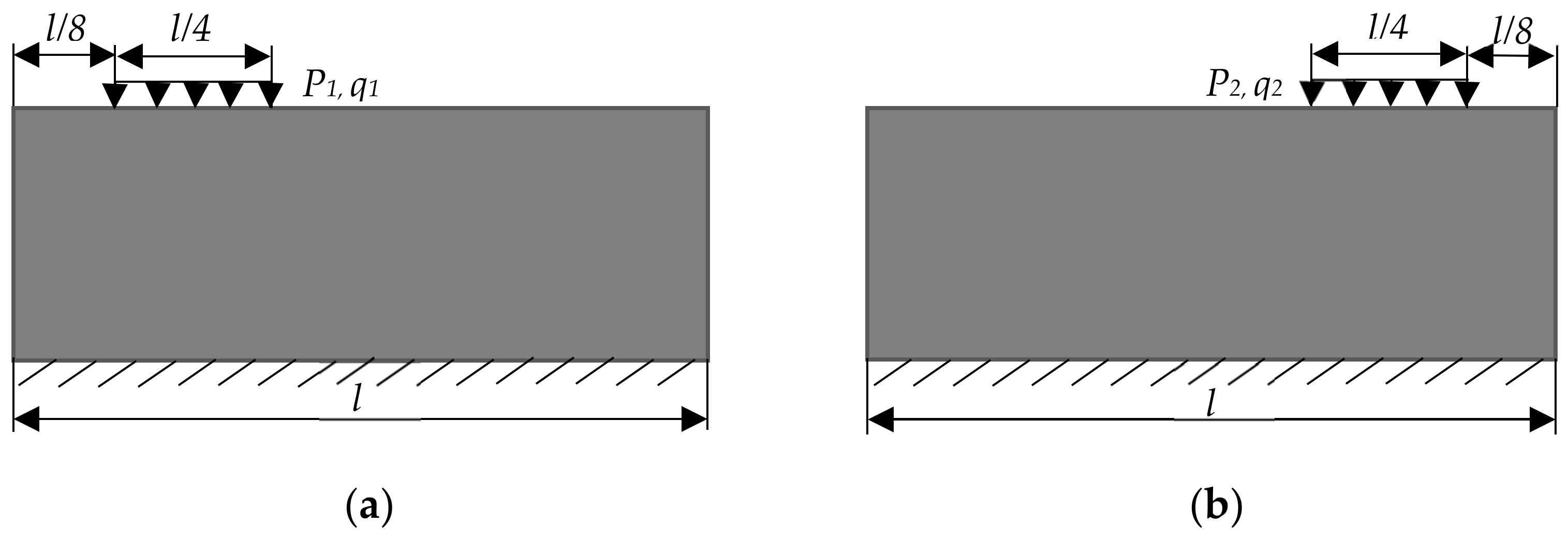
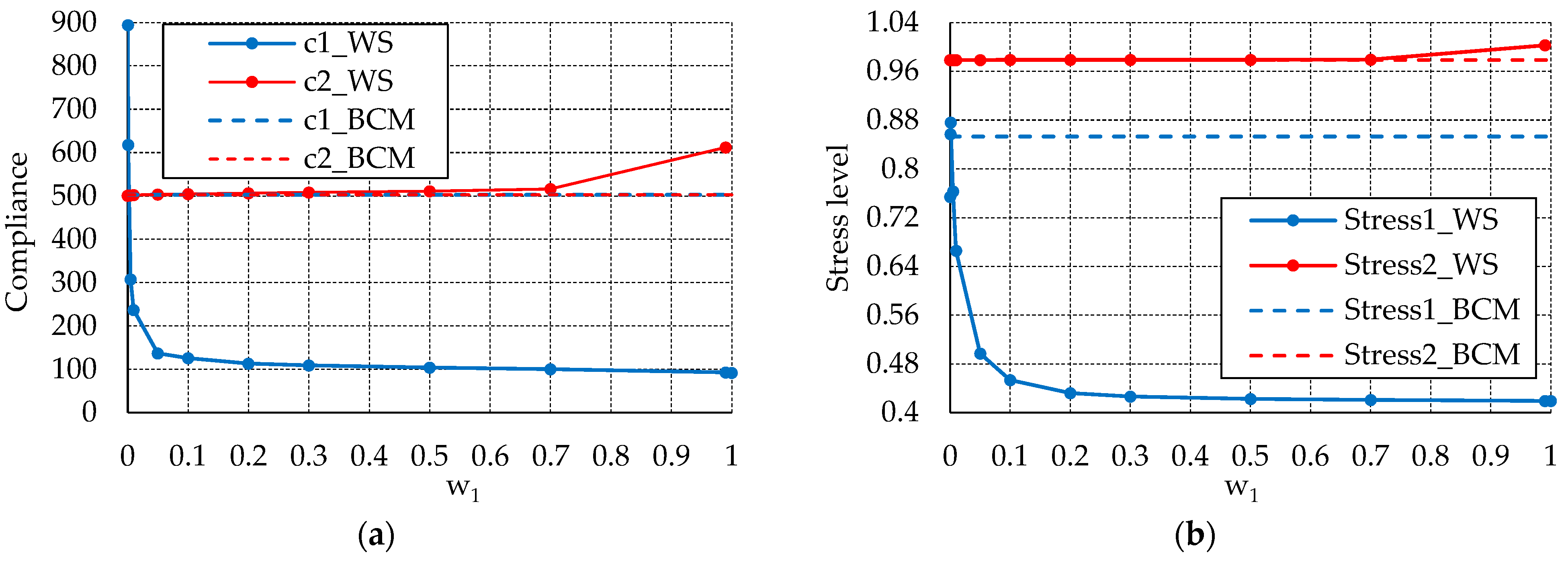
5.2. Loads Are Borne by a Local Region of the Structure
5.2.1. Problem 3
5.2.2. Problem 4
6. Conclusions
Author Contributions
Funding
Institutional Review Board Statement
Informed Consent Statement
Data Availability Statement
Conflicts of Interest
References
- Bendsøe, M.P.; Sigmund, O. Topology Optimization—Theory, Methods and Applications; Springer Science & Business Media: Berlin/Heidelberg, Germany, 2003. [Google Scholar]
- Bendsøe, M.P.; Kikuchi, N. Generating optimal topologies in structural design using a homogenization method. Comput. Methods Appl. Mech. Eng. 1998, 71, 197–224. [Google Scholar] [CrossRef]
- Suzuki, K.; Kikuchi, N. A homogenization method for shape and topology optimization. Comput. Methods Appl. Mech. Eng. 1991, 93, 291–318. [Google Scholar] [CrossRef]
- Torigaki, T.; Hagiwara, I.; Kitagawa, Y.; Ueda, M.; Ma, Z.D.; Kikuchi, N. Development and application of a shape-topology optimization system using a homogenization method. SAE Trans. 1994, 103, 1217–1223. [Google Scholar] [CrossRef]
- Allaire, G.; Belhachmi, Z.; Jouve, F. The homogenization method for topology and shape optimization. Single and multiple loads case. Rev. Eur. Élém. Finis 1996, 5, 649–672. [Google Scholar] [CrossRef]
- Groen, J.P.; Sigmund, O. Homogenization-based topology optimization for high-resolution manufacturable microstructures. Int. J. Numer. Methods Eng. 2018, 113, 1148–1163. [Google Scholar] [CrossRef]
- Xie, Y.M.; Steven, G.P. Shape and layout optimization via an evolutionary procedure. In Proceedings of the International Conference on Computational Engineering Science, Hong Kong, 17–22 December 1992; Volume 471. [Google Scholar]
- Xie, Y.M.; Steven, G.P. A simple evolutionary procedure for structural Optimization. Compurers Struct. 1993, 49, 885–896. [Google Scholar] [CrossRef]
- Huang, X.; Xie, Y.M. A further review of ESO type methods for topology optimization. Struct. Multidiscip. Optim. 2010, 41, 671–683. [Google Scholar] [CrossRef]
- Yang, X.Y.; Xie, Y.M.; Steven, G.P.; Querin, O.M. Bidirectional evolutionary method for stiffness optimisation. In Proceedings of the 7th AIAA/USAF/NASA/ISSMO Symposium on Multidisciplinary Analysis and Optimization, St. Louis, MO, USA, 2–4 September 1999; Volume 37, pp. 1483–1488. [Google Scholar] [CrossRef]
- Querin, O.M.; Young, V.; Steven, G.P.; Xie, Y.M. Computational efficiency and validation of bi-directional evolutionary structural optimization. Comput. Methods Appl. Mech. Eng. 2000, 189, 559–573. [Google Scholar] [CrossRef]
- Huang, X.; Xie, Y.M.; Burry, M.C. A new algorithm for bi-directional evolutionary structural optimization. JSME Int. J. Ser. C Mech. Syst. Mach. Elem. Manuf. 2007, 49, 1091–1099. [Google Scholar] [CrossRef]
- Wang, M.Y.; Zhou, S. Phase field: A variational method for structural topology optimization. Comput. Model. Eng. Sci. 2004, 6, 547–566. [Google Scholar] [CrossRef]
- Takezawa, A.; Nishiwaki, S.; Kitamura, M. Shape topology optimization based on the phase field method sensitivity analysis. J. Comput. Phys. 2010, 229, 2697–2718. [Google Scholar] [CrossRef]
- Luise, B.; Harald, G.; Lavinia, S.; Tarin, S.; Vanessa, S.A.V. Phase-field Approaches to Structural Topology Optimization. Constrained Optim. Optim. Control Partial Differ. Equ. 2012, 160, 245–256. [Google Scholar] [CrossRef]
- Blank, L.; Garcke, H.; Hassan Farshbaf-Shaker, M.; Styles, V. Relating phase field and sharp interface approaches to structural topology optimization. ESAIM—Control Optim. Calc. Var. 2014, 20, 1025–1058. [Google Scholar] [CrossRef]
- Auricchio, F.; Bonetti, E.; Carraturo, M.; Hömberg, D.; Reali, A.; Rocca, E. A phase-field-based graded-material topology optimization with stress constraint. Math. Models Methods Appl. Sci. 2020, 30, 1461–1483. [Google Scholar] [CrossRef]
- Osher, S.J.; Santosa, F. Level Set Methods for Optimization Problems Involving Geometry Constraints, I. Frequencies of a Two-Density Inhomogeneous Drum. J. Comput. Phys. 2001, 171, 272–288. [Google Scholar] [CrossRef]
- Allaire, G.; Jouve, F.; Toader, A.M. A level-set method for shape optimization, C.R. Acad. Sci. Paris. 2002, 334, 1125–1130. [Google Scholar] [CrossRef]
- Van Dijk, N.P.; Yoon, G.H.; Van Keulen, F.; Langelaar, M. A level-set based topology optimization using the element connectivity parameterization method. Struct. Multidiscip. Optim. 2010, 42, 269–282. [Google Scholar] [CrossRef]
- Wei, P.; Li, Z.; Li, X.; Wang, M.Y. An 88-line MATLAB code for the parameterized level set method based topology optimization using radial basis functions. Struct. Multidiscip. Optim. 2018, 58, 831–849. [Google Scholar] [CrossRef]
- Wei, P.; Paulino, G.H. A parameterized level set method combined with polygonal finite elements in topology optimization. Struct. Multidiscip. Optim. 2020, 61, 1913–1928. [Google Scholar] [CrossRef]
- Cui, M.; Luo, C.; Li, G.; Pan, M. The parameterized level set method for structural topology optimization with shape sensitivity constraint factor. Eng. Comput. 2021, 37, 855–872. [Google Scholar] [CrossRef]
- Lin, Y.; Zhu, W.; Li, J.; Ke, Y. Structural topology optimization using a level set method with finite difference updating scheme. Struct. Multidiscip. Optim. 2021, 63, 1839–1852. [Google Scholar] [CrossRef]
- Guo, X.; Zhang, W.; Zhong, W. Doing topology optimization explicitly geometrically-a new moving morphable components based framework. J. Appl. Mech. Trans. ASME 2014, 81, 081009. [Google Scholar] [CrossRef]
- Zhang, W.; Yuan, J.; Zhang, J.; Guo, X. A new topology optimization approach based on Moving Morphable Components (MMC) and the ersatz material model. Struct. Multidiscip. Optim. 2016, 53, 1243–1260. [Google Scholar] [CrossRef]
- Bendsøe, M.P. Optimal shape design as a material distribution problem. Struct. Optim. 1989, 1, 193–202. [Google Scholar] [CrossRef]
- Sigmund, O. On the Design of Compliant Mechanisms Using Topology Optimization. J. Struct. Mech. 1997, 25, 493–524. [Google Scholar] [CrossRef]
- Sigmund, O. A 99 line topology optimization code written in matlab. Struct. Multidiscip. Optim. 2001, 21, 120–127. [Google Scholar] [CrossRef]
- Andreassen, E.; Clausen, A.; Schevenels, M.; Lazarov, B.S.; Sigmund, O. Efficient topology optimization in MATLAB using 88 lines of code. Struct. Multidiscip. Optim. 2011, 43, 1–16. [Google Scholar] [CrossRef]
- Ma, J.; He, Y.; Zhao, Z.L.; Xie, Y.M. Topology optimization of ribbed slabs and shells. Eng. Struct. 2023, 277, 115454. [Google Scholar] [CrossRef]
- Golecki, T.; Gomez, F.; Carrion, J.; Spencer, B.F. Bridge topology optimization considering stochastic moving traffic. Eng. Struct. 2023, 292, 116498. [Google Scholar] [CrossRef]
- Shah, V.; Pamwar, M.; Sangha, B.; Kim, I.Y. All-terrain vehicle chassis design using multi-material topology optimization. Struct. Multidiscip. Optim. 2023, 66, 45. [Google Scholar] [CrossRef]
- Min, S.; Nishiwaki, S.; Kikuchi, N. Unified topology design of static and vibrating structures using multiobjective optimization. Comput. Struct. 2000, 75, 93–116. [Google Scholar] [CrossRef]
- Li, Y.; Yang, Q.; Chang, T.; Qin, T.; Wu, F. Multi-load cases topological optimization by weighted sum method based on load case severity degree and ideality. Adv. Mech. Eng. 2020, 12, 1–15. [Google Scholar] [CrossRef]
- Diaz, A.R.; Bendsoe, M.P. Shape optimization of structures for multiple loading conditions using a homogenization method. Struct. Optim. 1992, 4, 17–22. [Google Scholar] [CrossRef]
- Bendsøe, M.P.; Diaz, A.R.; Lipton, R.; Taylor, J.E. Optimal design of material properties and material distribution for multiple loading conditions. Int. J. Numer. Methods Eng. 1995, 38, 1149–1170. [Google Scholar] [CrossRef]
- Krog, L.; Tucked, A.; Kemp, M.; Boyd, R. Topology optimization of aircraft wing box ribs. In Proceedings of the 10th AIAA/ISSMO Multidisciplinary Analysis and Optimization Conference, Albany, NY, USA, 30 August–1 September 2004; Volume 3, pp. 2020–2030. [Google Scholar] [CrossRef]
- Pedersen, P. Aspects of 3D Shape and Topology Optimization with Multiple Load Cases. In Proceedings of the III European Conference on Computational Mechanics, Lisbon, Portugal, 5–8 June 2006; Springer: Dordrecht, The Netherlands, 2006; p. 492. [Google Scholar] [CrossRef]
- Marler, R.T.; Arora, J.S. The weighted sum method for multi-objective optimization: New insights. Struct. Multidiscip. Optim. 2010, 41, 853–862. [Google Scholar] [CrossRef]
- Sun, Y.; Lueth, T.C. Enhancing Torsional Stiffness of Continuum Robots Using 3-D Topology Optimized Flexure Joints. IEEE/ASME Trans. Mechatron. 2023, 28, 1844–1852. [Google Scholar] [CrossRef]
- Dämmer, G.; Gablenz, S.; Neumann, R.; Major, Z. Design, Topology Optimization, and Additive Manufacturing of a Pneumatically Actuated Lightweight Robot. Actuators. 2023, 12, 266. [Google Scholar] [CrossRef]
- Guo, Y.; Du, Z.; Liu, C.; Zhang, W.; Xue, R.; Guo, Y.; Tang, S.; Guo, X. Explicit topology optimization of three-dimensional geometrically nonlinear structures. Acta Mech. Sin. 2023, 39, 423084. [Google Scholar] [CrossRef]
- Rong, X.; Zheng, J.; Jiang, C. Topology optimization for structures with bi-modulus material properties considering displacement constraints. Comput. Struct. 2023, 276, 106952. [Google Scholar] [CrossRef]
- Chen, M.; Zuo, W.; Chen, Y.; Zhao, O.; Cheng, B. Parametric topology optimization design and analysis of additively manufactured joints in spatial grid structures. Eng. Struct. 2024, 300, 117123. [Google Scholar] [CrossRef]
- Haug, E.J.; Arora, J.S. Applied Optimal Design; J. Wiley and Sons: New York, NY, USA, 1979. [Google Scholar]
- Achtziger, W. Multiple-load truss topology sizing optimization: Some properties of minimax compliance. J. Optim. Theory Appl. 1998, 98, 255–280. [Google Scholar] [CrossRef]
- Rao, S.S. Game theory approach for multiobjective structural optimization. Comput. Struct. 1987, 25, 119–127. [Google Scholar] [CrossRef]
- Tseng, C.H.; Lu, T.W. Minimax multiobjective optimization in structural design. Int. J. Numer. Methods Eng. 1990, 30, 1213–1228. [Google Scholar] [CrossRef]
- Coello, C.A.C. Using the min-max method to solve multiobjective optimization problems with genetic algorithms. In Progress in Artificial Intelligence—IBERAMIA 98. IBERAMIA 1998; Lecture Notes in Computer Science; Springer: Berlin/Heidelberg, Germany, 1998; Volume 1484, pp. 303–313. [Google Scholar] [CrossRef]
- Cherkaev, E.; Cherkaev, A. Principal Compliance Robust Optimal Design. J. Elast. 2003, 72, 71–98. [Google Scholar] [CrossRef]
- Cherkaev, E.; Cherkaev, A. Minimax optimization problem of structural design. Comput. Struct. 2008, 86, 1426–1435. [Google Scholar] [CrossRef]
- Lógó, J.; Balogh, B.; Pintér, E. Topology optimization considering multiple loading. Comput. Struct. 2018, 207, 233–244. [Google Scholar] [CrossRef]
- Nowak, M.; Sokołowski, J.; Żochowski, A. Biomimetic Approach to Compliance Optimization Multiple Load Cases. J. Optim. Theory Appl. 2020, 184, 210–225. [Google Scholar] [CrossRef]
- Haimes, Y.V.; Lasdon, L.S.; Wismer, D.A. On a bicriterion formation of the problems of integrated system identification and system optimization. IEEE Trans. Syst. Man Cybern 1971, SMC-1, 296–297. [Google Scholar] [CrossRef]
- Mavrotas, G. Effective implementation of the ε-constraint method in Multi-Objective Mathematical Programming problems. Appl. Math. Comput. 2009, 213, 455–465. [Google Scholar] [CrossRef]
- Chircop, K.; Zammit-Mangion, D. On Epsilon-Constraint Based Methods for the Generation of Pareto Frontiers. J. Mech. Eng. Autom. 2013, 3, 279–289. [Google Scholar]
- Jaouadi, Z.; Lahmer, T. Topology optimization of structures subjected to multiple load cases by introducing the Epsilon constraint method. In Proceedings of the Digital Proceedings, International Conference on the Applications of Computer Science and Mathematics in Architecture and Civil Engineering, Weimar, CA, USA, 20–22 July 2015; pp. 84–90. [Google Scholar] [CrossRef]
- Hübner, D.; Wein, F.; Stingl, M. Two-scale optimization of graded lattice structures respecting buckling on micro- and macroscale. Struct. Multidiscip. Optim. 2023, 66, 163. [Google Scholar] [CrossRef]
- Azegami, H. Shape Optimization Problems; Springer: Singapore, 2020. [Google Scholar]
- Luo, Z.; Yang, J.; Chen, L.-P.; Zhang, Y.-Q.; Abdel-Malek, K. A new hybrid fuzzy-goal programming scheme for multi-objective topological optimization of static and dynamic structures under multiple loading conditions. Struct. Multidiscip. Optim. 2006, 31, 26–39. [Google Scholar] [CrossRef]
- Kumar, P. HoneyTop90: A 90-line MATLAB code for topology optimization using honeycomb tessellation. Optim. Eng. 2003, 24, 1433–1460. [Google Scholar] [CrossRef]
- Bendsoe, M.P.; Olhoff, N.; Taylor, J.E. AVariational Formulation for Multicriteria Structural Optimization. J. Struct. Mech. 1983, 11, 523–544. [Google Scholar] [CrossRef]
- Olhoff, N. Multicriterion structural optimization via bound formulation and mathematical programming. Struct. Optim. 1989, 1, 11–17. [Google Scholar] [CrossRef]
- Lasdon, L.S.; Waren, A.D.; Sarkar, S.; Palacios, F. Solving the Pooling Problem Using Generalized Reduced Gradient and Successive Linear Programming Algorithms. ACM Sigmap Bull. 1979, 27, 9–15. [Google Scholar] [CrossRef]
- Nocedal, J.; Wright, S.J. Numerical Optimization; Springer: New York, NY, USA, 2006. [Google Scholar]
- Liu, J.; Gaynor, A.T.; Chen, S.; Kang, Z.; Suresh, K.; Takezawa, A.; Li, L.; Kato, J.; Tang, J.; Wang, C.C.L.; et al. Current and future trends in topology optimization for additive manufacturing. Struct. Multidiscip. Optim. 2018, 57, 2457–2483. [Google Scholar] [CrossRef]
- Subedi, S.C.; Verma, C.S.; Suresh, K. A review of methods for the geometric post-processing of topology optimized models. J. Comput. Inf. Sci. Eng. 2020, 20, 060801. [Google Scholar] [CrossRef]
- Stankiewicz, G.; Dev, C.; Steinmann, P. Coupled topology and shape optimization using an embedding domain discretization method. Struct. Multidiscip. Optim. 2021, 64, 2687–2707. [Google Scholar] [CrossRef]


| Method | |||
|---|---|---|---|
| TEWS | 61.17191 | 52.23056 | 85.39076 |
| BCM | 76.93185 | 77.27681 | 77.27835 |
| Method | |||
|---|---|---|---|
| TEWS | 30.26961 | 285.3740 | 93.13086 |
| BCM | 63.27235 | 271.6586 | 231.3640 |
| Method | Stress Level 1 | Stress Level 2 | ||
|---|---|---|---|---|
| TEWS | 40.36 | 46.96 | 0.1435 | 0.1642 |
| BCM | 44.42 | 44.43 | 0.1623 | 0.1514 |
| Load Combination | Method | Topology | Stress Level 1 | Stress Level 2 | ||
|---|---|---|---|---|---|---|
| , | TEWS (Stage 1) |  | 3.44 | 43.37 | 0.050 | 0.153 |
| BCM (Stage 2) |  | 41.94 | 41.94 | 0.053 | 0.151 | |
| , | TEWS (Stage 1) |  | 15.64 | 45.07 | 0.118 | 0.158 |
| BCM (Stage 2) |  | 42.43 | 42.43 | 0.135 | 0.152 | |
| , | TEWS (Stage 1) |  | 40.36 | 46.96 | 0.143 | 0.164 |
| BCM (Stage 2) |  | 44.42 | 44.43 | 0.162 | 0.151 | |
| , | TEWS (Stage 1) |  | 48.37 | 48.37 | 0.159 | 0.159 |
| BCM (Stage 2) |  | 48.37 | 48.37 | 0.159 | 0.159 |
| Method | Stress Level 1 | Stress Level 2 | ||
|---|---|---|---|---|
| TEWS | 18.005 | 339.063 | 0.08307 | 0.16844 |
| BCM | 328.697 | 328.702 | 0.11578 | 0.16400 |
| Method | Stress Level 1 | Stress Level 2 | ||
|---|---|---|---|---|
| TEWS | 41.03794 | 316.71307 | 0.13203 | 0.17372 |
| BCM | 300.23040 | 300.23161 | 0.21627 | 0.15325 |
| Load Combination | Method | Topology | Stress Level 1 | Stress Level 2 | ||
|---|---|---|---|---|---|---|
| , | TEWS (Stage 1) |  | 18.00 | 339.06 | 0.083 | 0.168 |
| BCM (Stage 2) |  | 328.70 | 328.70 | 0.116 | 0.164 | |
| , | TEWS (Stage 1) |  | 41.04 | 316.71 | 0.132 | 0.173 |
| BCM (Stage 2) |  | 300.23 | 300.23 | 0.216 | 0.153 | |
| , | TEWS (Stage 1) |  | 129.94 | 235.84 | 0.223 | 0.190 |
| BCM (Stage 2) |  | 196.70 | 196.70 | 0.291 | 0.143 | |
| , | TEWS (Stage 1) |  | 254.30 | 154.19 | 0.299 | 0.183 |
| BCM (Stage 2) |  | 206.89 | 206.841 | 0.262 | 0.274 | |
| , | TEWS (Stage 1) |  | 341.27 | 121.18 | 0.344 | 0.178 |
| BCM (Stage 2) |  | 285.97 | 285.76 | 0.302 | 0.337 | |
| , | TEWS (Stage 1) |  | 448.23 | 91.66 | 0.399 | 0.180 |
| BCM (Stage 2) |  | 379.85 | 379.86 | 0.350 | 0.321 | |
| , | TEWS (Stage 1) |  | 546.24 | 77.81 | 0.424 | 0.187 |
| BCM (Stage 2) |  | 481.98 | 481.98 | 0.391 | 0.184 |
| Load Combination | Method | Topology | Stress Level 1 | Stress Level 2 | ||
|---|---|---|---|---|---|---|
| , .0 | TEWS |  | 49.56 | 662.47 | 0.285 | 1.119 |
| BCM |  | 635.91 | 654.71 | 0.614 | 1.118 | |
| , | TEWS |  | 104.04 | 511.08 | 0.423 | 0.9789 |
| BCM |  | 503.04 | 503.04 | 0.853 | 0.9787 | |
| , | TEWS |  | 271.911 | 271.911 | 0.7007 | 0.7007 |
| BCM |  | 271.911 | 271.911 | 0.7007 | 0.7007 | |
| , | TEWS |  | 662.47 | 49.56 | 1.119 | 0.285 |
| BCM |  | 654.71 | 635.91 | 1.118 | 0.614 | |
| , | TEWS |  | 833.06 | 14.75 | 1.2584 | 0.1626 |
| BCM |  | 827.99 | 806.55 | 1.2583 | 0.3133 |
| Load Combination | Method | Topology | Stress Level 1 | Stress Level 2 | ||
|---|---|---|---|---|---|---|
| , .0 | TEWS |  | 11.425 | 65.029 | 0.04171 | 0.06162 |
| BCM |  | 58.655 | 59.568 | 0.22641 | 0.05960 | |
| , | TEWS |  | 18.469 | 53.520 | 0.04483 | 0.05567 |
| BCM |  | 46.853 | 46.844 | 0.13768 | 0.05380 | |
| , | TEWS |  | 25.433 | 43.472 | 0.04648 | 0.04942 |
| BCM |  | 37.698 | 37.665 | 0.08742 | 0.04704 | |
| , | TEWS |  | 33.863 | 33.863 | 0.04952 | 0.04952 |
| BCM |  | 33.863 | 33.863 | 0.04952 | 0.04952 | |
| , | TEWS |  | 38.400 | 29.768 | 0.048445 | 0.04744 |
| BCM |  | 34.779 | 34.776 | 0.04519 | 0.06684 | |
| , | TEWS |  | 77.637 | 5.200 | 0.06717 | 0.03589 |
| BCM |  | 75.793 | 70.078 | 0.06630 | 0.18600 |
Disclaimer/Publisher’s Note: The statements, opinions and data contained in all publications are solely those of the individual author(s) and contributor(s) and not of MDPI and/or the editor(s). MDPI and/or the editor(s) disclaim responsibility for any injury to people or property resulting from any ideas, methods, instructions or products referred to in the content. |
© 2023 by the authors. Licensee MDPI, Basel, Switzerland. This article is an open access article distributed under the terms and conditions of the Creative Commons Attribution (CC BY) license (https://creativecommons.org/licenses/by/4.0/).
Share and Cite
Pham-Truong, T.; Kawamura, Y.; Okada, T. Bisection Constraint Method for Multiple-Loading Conditions in Structural Topology Optimization. Appl. Sci. 2023, 13, 13005. https://doi.org/10.3390/app132413005
Pham-Truong T, Kawamura Y, Okada T. Bisection Constraint Method for Multiple-Loading Conditions in Structural Topology Optimization. Applied Sciences. 2023; 13(24):13005. https://doi.org/10.3390/app132413005
Chicago/Turabian StylePham-Truong, Thi, Yasumi Kawamura, and Tetsuo Okada. 2023. "Bisection Constraint Method for Multiple-Loading Conditions in Structural Topology Optimization" Applied Sciences 13, no. 24: 13005. https://doi.org/10.3390/app132413005
APA StylePham-Truong, T., Kawamura, Y., & Okada, T. (2023). Bisection Constraint Method for Multiple-Loading Conditions in Structural Topology Optimization. Applied Sciences, 13(24), 13005. https://doi.org/10.3390/app132413005