Robust Elastic Full-Waveform Inversion Based on Normalized Cross-Correlation Source Wavelet Inversion

Abstract

The elastic full-waveform inversion (EFWI) method efficiently utilizes the amplitude, phase, and travel time information present in multi-component seismic recordings to create detailed parameter models of subsurface structures. Within full-waveform inversion (FWI), accurate source wavelet estimation significantly impacts both the convergence and final result quality. The source wavelet, serving as the initial condition for the wave equation’s forward modeling algorithm, directly influences the matching degree between observed and synthetic data. This study introduces a novel method for estimating the source wavelet utilizing cross-correlation norm elastic waveform inversion (CNEWI) and outlines the EFWI algorithm flow based on this CNEWI source wavelet inversion. The CNEWI method estimates the source wavelet by employing normalized cross-correlation processing on near-offset direct waves, thereby reducing the susceptibility to strong amplitude interference such as bad traces and surface wave residuals. The proposed CNEWI method exhibits a superior computational efficiency compared to conventional L2-norm waveform inversion for source wavelet estimation. Numerical experiments, including in ideal scenarios, with seismic data with bad traces, and with multi-component data, validate the advantages of the proposed method in both source wavelet estimation and EFWI compared to the traditional inversion method.

1. Introduction

The full-waveform inversion (FWI) method can build high-precision velocity models of subsurface media using observed seismic data [1,2]. The FWI method was originally proposed based on acoustic media [3,4]. By matching the synthetic data simulated by the scalar acoustic wave equation with the observed data, the FWI method finally obtains a high-resolution P-wave velocity model of an underground medium [5]. The key point of the FWI algorithm is the calculation of the derivative of the objective function with respect to the model parameter to be determined, which is known as the gradient of FWI [6]. The adjoint-state method reduces the computational complexity of the gradient calculation, making practical application of the FWI algorithm possible [7]. In recent years, acoustic FWI has successfully inverted industrial-scale real 3D marine data [8] and refracted waves in ocean bottom node data [9]. However, modeling of elastic wave propagation through elastodynamic theory is required for reflection analysis [10,11]. In real cases, when seismic waves propagate in underground media, if they encounter a reflecting interface, energy conversion will occur and converted waves will be generated. The elastic wave equation can better describe the actual wavefield propagation characteristics and laws than the acoustic wave equation [12,13].

The elastic full-waveform inversion (EFWI) method was first implemented in 1986 [14] and practical data applications appeared in 1990 [15]. Due to the consideration of multiple parameters, the nonlinearity of EFWI is stronger than that of acoustic FWI and the computational complexity is higher [16,17]. To reduce the nonlinearity of EFWI, a good strategy is to choose a more convex objective function, which can help to mitigate the cycle-skipping issue during inversion [18]. The objective function of FWI is initially the L2 norm of the residuals between observed and synthetic data. When the travel time difference between the synthetic and observed data is greater than half a cycle, the cycle-skipping phenomenon will occur, resulting in the inversion falling into a local minimum. In addition to the differences in velocity models, many factors may result in cycle skipping during inversion, such as amplitude errors caused by data acquisition or processing, source wavelet errors, etc. To mitigate the cycle-skipping issue caused by amplitude errors, the cross-correlation objective function was proposed [19]. Using normalized global cross-correlation to construct the objective function can overcome the impact of the entire trace amplitude errors on FWI. The local cross-correlation objective function can further overcome the impact of local amplitude errors on inversion [20]. In addition, Laplace domain waveform inversion [21] and envelope inversion [22,23] can construct large-scale velocity models of subsurface media when seismic data lack low-frequency information. The multiscale FWI strategy based on these methods can obtain high-precision velocity models [24]. Oh and Alkhalifah [25] combined the cross-correlation operation and the envelope operation to construct a new objective function, which can simultaneously overcome the effects of amplitude errors and missing low frequencies on the inversion. Zhang et al. [26] extended this method to elastic media and added the convolution operation to construct a new objective function, simultaneously overcoming the effects of amplitude errors, missing low frequencies, and source wavelet inaccuracy on the inversion.

The source wavelet is another key factor affecting the accuracy of EFWI. For frequency-domain FWI, source wavelet estimation can be performed relatively simply according to the L2 norm inversion method [27,28]. During the inversion process, the source wavelet needs to be updated simultaneously with the velocity. To overcome the impact of source inaccuracy on inversion, source-independent inversion strategies were first proposed in frequency-domain FWI, including convolution-based inversion methods [29,30] and deconvolution-based inversion methods [31,32,33,34]. In the time domain, source-independent inversion methods are usually constructed based on convolved wavefields [35]. This method can obtain good inversion results under ideal circumstances, and the same is true for EFWI [36]. However, the convolved wavefield method may amplify low-frequency noise due to the convolution operation used. Moreover, when there are bad traces in the data, this method cannot avoid their impact on the final inversion results. In the time domain, the waveform inversion method based on the L2 norm objective function can still be used to invert the source wavelet function [37,38]. This kind of source wavelet inversion method has been used in FWI and reverse time migration [39,40,41]. However, just like traditional FWI, this source wavelet inversion method will also be affected by many factors, among which the amplitude error is one of the key factors [42]. When there are amplitude errors or bad traces in the seismic data, inversion will be significantly affected. The above research is mainly focused on acoustic media. This paper proposes a source wavelet estimation method using multi-component seismic data in elastic media.

In this paper, we first review the basic principles of EFWI and the source wavelet inversion method based on the L2 norm objective function. Aiming at solving the effects of bad traces, surface wave residuals, and amplitude errors on source wavelet inversion in elastic media, a source wavelet inversion method using multi-component seismic data based on the cross-correlation elastic waveform inversion method is proposed. Finally, numerical tests are conducted to verify the effectiveness of the proposed method.

2. Methods

2.1. Elastic Full-Waveform Inversion (EFWI)

EFWI can provide high-resolution multi-parameter models of underground media by fitting the full wave information of multi-component seismic data. The objective function of EFWI using multi-component seismic data can be written as follows [12],

$${\sigma }_1\left(\lambda ,\mu ,v_p,v_s\right)={\displaystyle \sum _i^{ns}{\displaystyle \sum _j^{nr}\left[{‖u_{i,j}^x\left(\lambda ,\mu ,v_p,v_s\right)-d_{i,j}^x‖}^2+{‖u_{i,j}^z\left(\lambda ,\mu ,v_p,v_s\right)-d_{i,j}^z‖}^2\right]}} ,$$

(1)

where ${\sigma }_1$ denotes the objective function value; $i$ and $j$ denote the source and receiver index, respectively; $ns$ and $nr$ denote the total number of sources and receivers, respectively; $u_{i,j}^x$ and $u_{i,j}^z$ denote the x- and z-component of the synthetic data in the time domain, respectively; $d_{i,j}^x$ and $d_{i,j}^z$ denote the x- and z-component of the observed data in the time domain, respectively; $\lambda$ and $\mu$ are lame constants; and $v_p$ and $v_s$ denote P-wave velocity and S-wave velocity, respectively. In Equation (1), the density parameter is assumed to be constant. Equation (1) represents the objective function, which assesses waveform matching by computing the L2-norm of the residuals between observed and synthetic data. Amplitude errors in the observed data can lead to waveform differences not solely attributable to the velocity model. Consequently, the inversion process may converge to a local minimum, impeding reliable inversion outcomes. To address this issue, employing an objective function reliant on cross-correlation operations proves advantageous, given that [19]

$${\sigma }_2\left(\lambda ,\mu ,v_p,v_s\right)={\displaystyle \sum _i^{ns}{\displaystyle \sum _j^{nr}\left[-{\widehat{u}}_{i,j}^x\left(\lambda ,\mu ,v_p,v_s\right)\cdot {\widehat{d}}_{i,j}^x-{\widehat{u}}_{i,j}^z\left(\lambda ,\mu ,v_p,v_s\right)\cdot {\widehat{d}}_{i,j}^z\right]}},$$

(2)

where ${\widehat{u}}_{i,j}^x$ and ${\widehat{u}}_{i,j}^z$ denote the normalized x- and z-component of the synthetic data, respectively, i.e., ${\widehat{u}}_{i,j}^x=u_{i,j}^x/‖u_{i,j}^x‖$, ${\widehat{u}}_{i,j}^z=u_{i,j}^z/‖u_{i,j}^z‖$, and ${\widehat{d}}_{i,j}^x$ and ${\widehat{d}}_{i,j}^z$ denote the normalized x- and z-component of the observed data, respectively, i.e., ${\widehat{d}}_{i,j}^x=d_{i,j}^x/‖d_{i,j}^x‖$, ${\widehat{d}}_{i,j}^z=d_{i,j}^z/‖d_{i,j}^z‖$. According to the adjoint-state method [7], the derivative of ${\sigma }_2$ with respect to the lame constants $\lambda$ and $\mu$ can be written as

$$\frac{\partial {\sigma }_2}{\partial \lambda }=-{\displaystyle {\int }_0^T\left(\frac{\partial u_x}{\partial x}+\frac{\partial u_z}{\partial z}\right)\left(\frac{\partial u_x^{+}}{\partial x}+\frac{\partial u_z^{+}}{\partial z}\right)dt},$$

(3)

$$\frac{\partial {\sigma }_2}{\partial \mu }=-{\displaystyle {\int }_0^T\left\{2\left(\frac{\partial u_x}{\partial x}\cdot \frac{\partial u_x^{+}}{\partial x}+\frac{\partial u_z}{\partial z}\cdot \frac{\partial u_z^{+}}{\partial z}\right)+\left(\frac{\partial u_z}{\partial x}+\frac{\partial u_x}{\partial z}\right)\left(\frac{\partial u_z^{+}}{\partial x}+\frac{\partial u_x^{+}}{\partial z}\right)\right\}dt,}$$

(4)

where $u_x$ and $u_z$ denote the x- and z-component of the source forward propagated wavefield, respectively, and $u_x^{+}$ and $u_z^{+}$ denote the x- and z-component of the adjoint source backward-propagated wavefield, respectively. The x- and z-component of the adjoint source can be calculated by

$$A_x=\frac{1}{‖u_{i,j}^x‖}\left[{\widehat{u}}_{i,j}^x\left({\widehat{u}}_{i,j}^x\cdot {\widehat{d}}_{i,j}^x\right)-{\widehat{d}}_{i,j}^x\right],$$

(5)

$$A_z=\frac{1}{‖u_{i,j}^z‖}\left[{\widehat{u}}_{i,j}^z\left({\widehat{u}}_{i,j}^z\cdot {\widehat{d}}_{i,j}^z\right)-{\widehat{d}}_{i,j}^z\right].$$

(6)

According to the petrophysics relationship, we can know that the P-wave velocity $v_p$ and the S-wave velocity $v_s$ can be calculated by

$$v_p=\sqrt{\frac{\lambda +2\mu }{\rho }},$$

(7)

$$v_s=\sqrt{\frac{\mu }{\rho }},$$

(8)

where $\rho$ denotes density. From Equations (7) and (8), we can easily obtain the formulas of $\lambda$ and $\mu$ as

$$\lambda =\rho v_p^2-2\rho v_s^2,$$

(9)

$$\mu =\rho v_s^2.$$

(10)

The derivative of the objective function ${\sigma }_2$ with respect to the P-wave velocity and S-wave velocity can be calculated by the chain rule as

$$\frac{\partial {\sigma }_2}{\partial v_p}=\frac{\partial {\sigma }_2}{\partial \lambda }\cdot \frac{\partial \lambda }{\partial v_p}=2\rho v_p\frac{\partial {\sigma }_2}{\partial \lambda },$$

(11)

$$\frac{\partial {\sigma }_2}{\partial v_s}=\frac{\partial {\sigma }_2}{\partial \lambda }\cdot \frac{\partial \lambda }{\partial v_s}+\frac{\partial {\sigma }_2}{\partial \mu }\cdot \frac{\partial \mu }{\partial v_s}=-4\rho v_s\frac{\partial {\sigma }_2}{\partial \lambda }+2\rho v_s\frac{\partial {\sigma }_2}{\partial \mu }.$$

(12)

Substituting Equations (3) and (4) into Equations (11) and (12), we can obtain the gradient formula of the P-wave velocity and S-wave velocity as

$$\frac{\partial {\sigma }_2}{\partial v_p}=-2\rho v_p{\displaystyle {\int }_0^T\left(\frac{\partial u_x}{\partial x}+\frac{\partial u_z}{\partial z}\right)\left(\frac{\partial u_x^{+}}{\partial x}+\frac{\partial u_z^{+}}{\partial z}\right)dt},$$

(13)

$$\begin{array}{ll}\frac{\partial {\sigma }_2}{\partial v_s}& =4\rho v_s{\displaystyle {\int }_0^T\left(\frac{\partial u_x}{\partial x}+\frac{\partial u_z}{\partial z}\right)\left(\frac{\partial u_x^{+}}{\partial x}+\frac{\partial u_z^{+}}{\partial z}\right)dt}\\ & -2\rho v_s{\displaystyle {\int }_0^T\left[2\left(\frac{\partial u_x}{\partial x}\frac{\partial u_x^{+}}{\partial x}+\frac{\partial u_z}{\partial z}\frac{\partial u_z^{+}}{\partial z}\right)+\left(\frac{\partial u_z}{\partial x}+\frac{\partial u_x}{\partial z}\right)\left(\frac{\partial u_z^{+}}{\partial x}+\frac{\partial u_x^{+}}{\partial z}\right)\right]dt}.\end{array}$$

(14)

There are many factors that can affect the EFWI effects, among which the source wavelet accuracy is important. The source wavelet is the initial condition of the forward simulation of the seismic wavefield, and the forward simulation is an important part of the FWI algorithm. Source wavelet errors can easily cause the inversion to fall into a local minimum. Therefore, accurate source wavelet estimation is very important for EFWI.

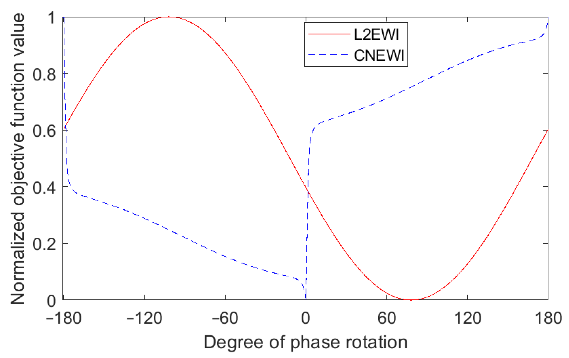
2.2. Source Wavelet Inversion Based on L2-Norm Elastic Waveform Inversion (L2EWI)

Assuming that the near-surface velocity model is relatively accurate, the source wavelet function can be obtained by using the direct wave waveform inversion method. Using near-offset multi-component direct waves to construct the L2 norm objective function, we can obtain

$${\sigma }_3\left(s\right)={\displaystyle \sum _i^{ns}{\displaystyle \sum _j^{nr}\left[{‖U_{i,j}^x\left(s\right)-D_{i,j}^x‖}^2+{‖U_{i,j}^z\left(s\right)-D_{i,j}^z‖}^2\right]}} ,$$

(15)

where $U$ and $D$ denote the synthetic direct waves and the observed direct waves, respectively, and $s$ denotes the source wavelet. According to the adjoint-state method, the derivative of the objective function ${\sigma }_3$ with respect to the source wavelet can be written as

$$\frac{\partial {\sigma }_3}{\partial s_i}={\displaystyle \sum _j^{nr}\left[{\left(\frac{\partial F}{\partial s_i}\right)}^T{\left(L^{-1}\right)}^T\left(U_{i,j}^x-D_{i,j}^x\right)+{\left(\frac{\partial F}{\partial s_i}\right)}^T{\left(L^{-1}\right)}^T\left(U_{i,j}^z-D_{i,j}^z\right)\right]},$$

(16)

where $s_i$ denotes the source wavelet function of the $i$th shot, $F$ denotes the source matrix, $L$ denotes the wavefield propagation operator, and the superscript T denotes transpose. It can be seen from Equation (16) that when the initial value of the inverted source wavelet is the zero vector, it is equivalent to backpropagating the observed data. This is the wavefield backpropagation source wavelet estimation method. Consequently, the wavefield backpropagation-derived source wavelet can serve as the initial wavelet in the L2EWI method. Given the capacity of the wavefield backpropagation algorithm to extract accurate phase information from the source wavelet, the resultant wavelet can be considered a dependable initial source wavelet. Nevertheless, similar to the L2 norm full-waveform inversion, the presence of amplitude errors in the observed data impacts the accuracy of the source wavelet estimated via Equation (16).

2.3. Source Wavelet Inversion by Cross-Correlation Norm Elastic Waveform Inversion (CNEWI)

In order to overcome the influences of source wavelet amplitude errors, which may be caused by surface wave interference, noise interference, data processing, etc., the following objective function can be constructed:

$${\sigma }_4\left(s\right)={\displaystyle \sum _i^{ns}{\displaystyle \sum _j^{nr}\left[-{\widehat{U}}_{i,j}^x\left(s\right)\cdot {\widehat{D}}_{i,j}^x-{\widehat{U}}_{i,j}^z\left(s\right)\cdot {\widehat{D}}_{i,j}^z\right]}},$$

(17)

where ${\widehat{U}}_{i,j}^x$ and ${\widehat{U}}_{i,j}^z$ denote the normalized x- and z-component of the synthetic direct waves, respectively, i.e., ${\widehat{U}}_{i,j}^x=U_{i,j}^x/‖U_{i,j}^x‖$, ${\widehat{U}}_{i,j}^z=U_{i,j}^z/‖U_{i,j}^z‖$, and ${\widehat{D}}_{i,j}^x$ and ${\widehat{D}}_{i,j}^z$ denote the normalized x- and z-component of the observed direct waves, respectively, i.e., ${\widehat{D}}_{i,j}^x=D_{i,j}^x/‖D_{i,j}^x‖$, ${\widehat{D}}_{i,j}^z=D_{i,j}^z/‖D_{i,j}^z‖$. The derivative of the objective function ${\sigma }_4$ with respect to the source wavelet function can be written as

$$\frac{\partial {\sigma }_4}{\partial s_i}={\displaystyle \sum _j^{nr}\left[{\left(\frac{\partial U_{i,j}^x}{\partial s_i}\right)}^T\frac{1}{‖U_{i,j}^x‖}\left({\widehat{U}}_{i,j}^x\left({\widehat{U}}_{i,j}^x\cdot {\widehat{D}}_{i,j}^x\right)-{\widehat{D}}_{i,j}^x\right)+{\left(\frac{\partial U_{i,j}^z}{\partial s_i}\right)}^T\frac{1}{‖U_{i,j}^z‖}\left({\widehat{U}}_{i,j}^z\left({\widehat{U}}_{i,j}^z\cdot {\widehat{D}}_{i,j}^z\right)-{\widehat{D}}_{i,j}^z\right)\right]}.$$

(18)

Utilizing the adjoint-state method, Equation (18) can be computed as follows:

$$\frac{\partial {\sigma }_4}{\partial s_i}={\displaystyle \sum _j^{nr}\left[{\left(\frac{\partial F}{\partial s_i}\right)}^T{\left(L^{-1}\right)}^T\frac{1}{‖U_{i,j}^x‖}\left({\widehat{U}}_{i,j}^x\left({\widehat{U}}_{i,j}^x\cdot {\widehat{D}}_{i,j}^x\right)-{\widehat{D}}_{i,j}^x\right)+{\left(\frac{\partial F}{\partial s_i}\right)}^T{\left(L^{-1}\right)}^T\frac{1}{‖U_{i,j}^z‖}\left({\widehat{U}}_{i,j}^z\left({\widehat{U}}_{i,j}^z\cdot {\widehat{D}}_{i,j}^z\right)-{\widehat{D}}_{i,j}^z\right)\right]}.$$

(19)

It can be seen that, compared with Equation (16), the gradient calculation of the CNEWI method just replaces the backpropagated residual terms with $\frac{1}{‖U_{i,j}^x‖}\left({\widehat{U}}_{i,j}^x\left({\widehat{U}}_{i,j}^x\cdot {\widehat{D}}_{i,j}^x\right)-{\widehat{D}}_{i,j}^x\right)$ and $\frac{1}{‖U_{i,j}^z‖}\left({\widehat{U}}_{i,j}^z\left({\widehat{U}}_{i,j}^z\cdot {\widehat{D}}_{i,j}^z\right)-{\widehat{D}}_{i,j}^z\right)$. Due to the normalization of the wavefield within the CNEWI method, choosing the zero vector as the initial source wavelet is deemed unsuitable. Similar to the L2EWI method, the CNEWI method can utilize the source wavelet obtained through the wavefield backpropagation method as its initial source wavelet.

2.4. Inversion Strategies

When performing EFWI, it is necessary to use multiscale inversion strategies and multi-component seismic data. Multiscale EFWI inverts sequentially from low frequency to high frequency, first constructing large-scale P-wave and S-wave velocity models and then constructing fine velocity models. Low-frequency data are more critical and can help overcome inversion instabilities caused by inaccurate initial models. When the low frequency in the original data is insufficient, methods such as envelope inversion can be used to extract the ultra-low frequency information for inversion, and then multiscale EFWI can be conducted. If the observed data are multi-component seismic data, all data components should be used when performing the inversion to reduce the multi-solution nature of the inversion and improve the inversion accuracy and resolution. However, if some data components are of poor quality, they should be removed to avoid introducing interference in the inversion.

Theoretically, inversion based on the cross-correlation objective function mainly uses the phase information of seismic data to overcome the influence of amplitude inaccuracy. Therefore, even if the CNEWI method cannot obtain accurate source wavelet amplitude information, it will not have a significant impact on subsequent EFWI, because the cross-correlation objective function can also be used in the EFWI process; this has been verified in the subsequent numerical examples.

There are some source-independent inversion strategies to overcome the effects of source wavelet errors on EFWI. In time-domain EFWI, the most common strategy is based on the convolved wavefields [26,35]. However, the convolution process may amplify noise in some cases because it is a multiplication process in the frequency domain. Also, for real seismic data from a common source, the convolution signal model is only an approximation. For far-offset data, the approximation effect is relatively poor. The reference trace selection will also affect source-independent inversion. Therefore, we chose to directly invert the source wavelet from the near-offset direct waves, which can mitigate the cycle-skipping caused by the source wavelet errors and improve the robustness of the EFWI process.

For elastic wave source wavelet inversion, the application of multi-component data can also theoretically improve the accuracy of the inversion. However, when the data are noisy or of poor quality, it is recommended to use single-component data inversion to avoid introducing interference. The initial source wavelet for both CNEWI and L2EWI inversion can use the source wavelet estimated by wavefield backpropagation. Since the method discussed in this paper uses near-offset direct waves for inversion, it is necessary to assume that the shallow velocity model is relatively accurate. Therefore, before performing CNEWI and L2EWI inversion, on the one hand, near-offset direct wave data should be intercepted, and on the other hand, a relatively accurate shallow velocity model should be obtained. Generally speaking, the velocity accuracy of first-arrival tomography can meet the requirements.

To test the cross-talk between the P-wave velocity and S-wave velocity of the CNEWI method, we conducted a numerical test using a simple elastic model. The true P-wave and S-wave velocity models are shown in Figure 1a and Figure 1b, respectively. There is a high-velocity layer in the model. The position of the layer is different in the P-wave velocity model and the S-wave velocity model. This may be rare in practice, but it is a good choice for the cross-talk test. The initial P-wave and S-wave velocity models are shown in Figure 1c and Figure 1d, respectively. The source wavelet is a Ricker wavelet with a dominant frequency of 20 Hz. EFWI with a normalized cross-correlation objective function was conducted. The P-wave velocity and S-wave velocity are updated simultaneously, and the result after 100 iterations is shown in Figure 1e,f. We can see that both the high-velocity layers in the P-wave velocity model and the S-wave velocity model are recovered well, which demonstrates that the P-wave velocity and S-wave velocity can be decoupled well during inversion.

3. Numerical Examples

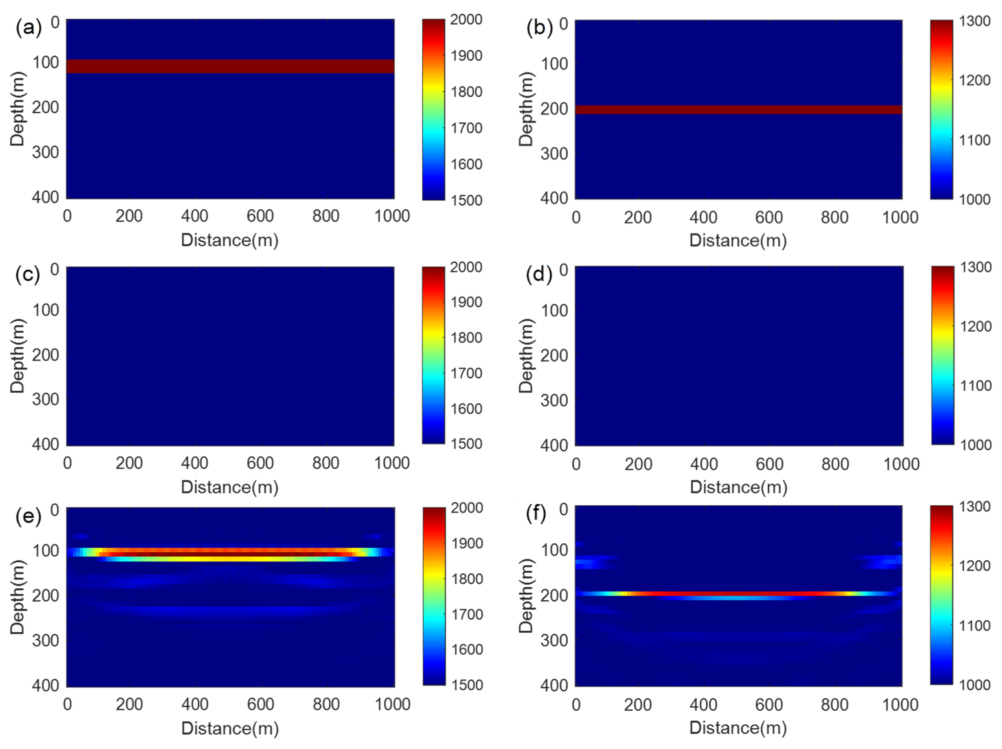
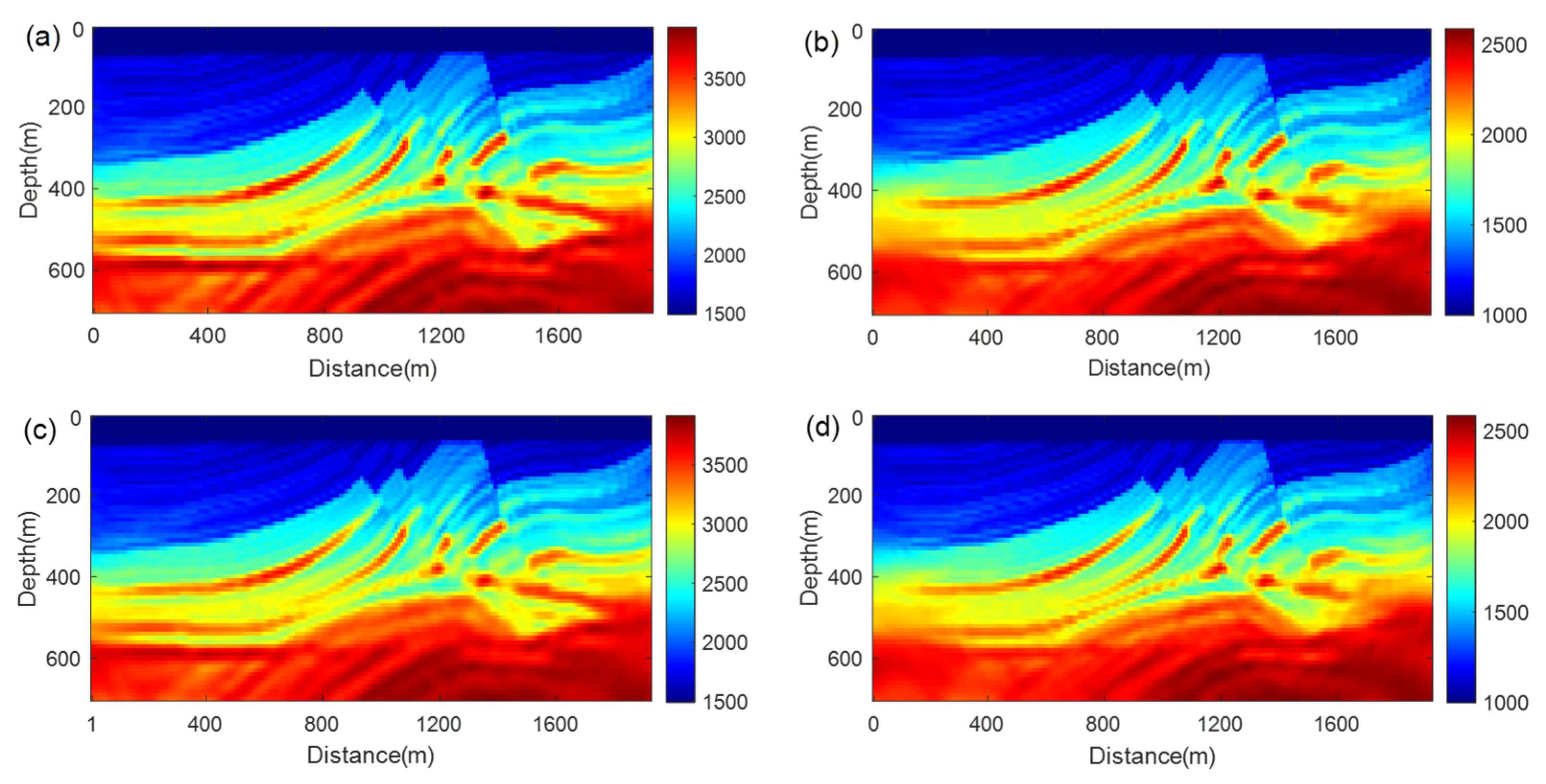
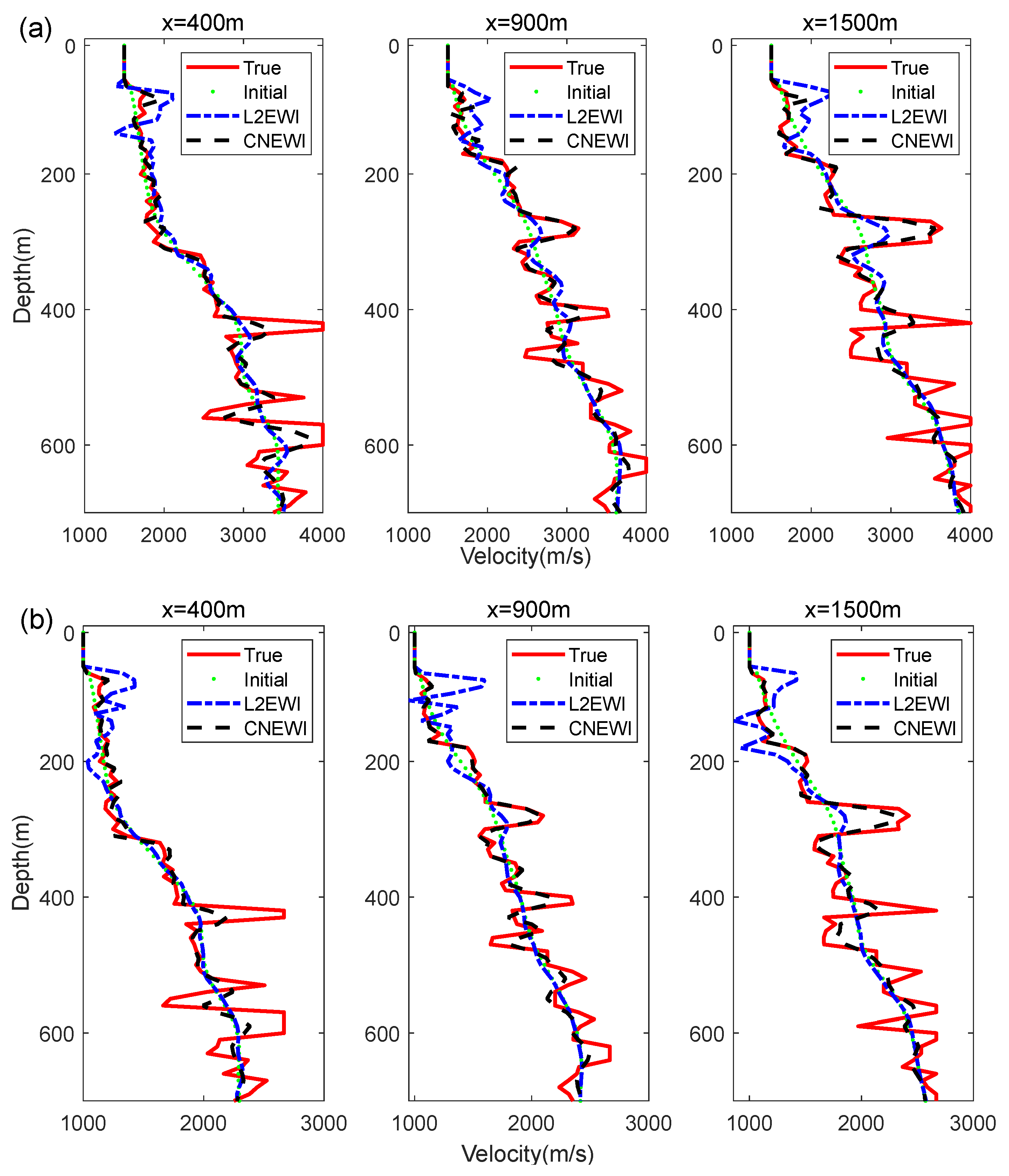
3.1. Inversion Effects in the Ideal Case

The effects of CNEWI source wavelet estimation and elastic full-waveform inversion under ideal conditions are discussed in this section. The model we used in the numerical tests is a modified Marmousi2 model [43]. The original model was rescaled, and the P-wave velocity and S-wave velocity models we used are shown in Figure 2a and Figure 2b, respectively. The S-wave velocity in the shallow part was set to non-zero values, because we mainly simulate a land seismic exploration case, which is more challenging for source wavelet inversion and FWI. One advantage of the proposed method is that it can overcome the effects of residual surface waves and near-offset bad traces on source wavelet inversion. In some cases, such as sand or soil, the velocity at the near surface can be treated as uniform. The primary focus of this paper revolves around examining the influence of source wavelet estimation on elastic full-waveform inversion. For this purpose, the initial velocity models here adopt the smooth velocity model, illustrated in Figure 3, which represents the achievable accuracy level in tomography. The observed seismic data were generated using a Ricker wavelet characterized by a dominant frequency of 20 Hz. Thirty-two sources were utilized with a source interval of 60 m. The data were sampled at intervals of 1 ms, spanning a recording time of 1.2 s. The observed data corresponding to a single shot are depicted in Figure 4, where Figure 4a,b represent the Z-component and X-component data, respectively. For inversion purposes, data within the 0.2 s timeframe were extracted. Both the L2EWI and CNEWI methods were applied to invert the source wavelet, and the resulting outcomes are presented in Figure 5. It is observed that, under ideal conditions, the L2EWI method accurately captures both the amplitude and phase information of the source wavelet, while the CNEWI method performs exceptionally well in extracting phase information. The inverted source wavelets were used to simulate direct waves, illustrated in Figure 6. Specifically, Figure 6a shows the Z-component direct wave record of the observed seismic data. Subsequently, Figure 6b,c displays the simulated direct wave data using the source wavelets inverted by the L2EWI and CNEWI methods, respectively. Notably, both simulated direct wave datasets align closely with the observed direct wave data, indicating the effectiveness of the source wavelet obtained through both methods. The changes in the objective functions of the two inversion methods are shown in Figure 7. Figure 7a shows the change in the objective function curves of the L2EWI method for inverting the 32-shot data, and Figure 7b shows the change in the objective function curves of the CNEWI method for inverting the 32-shot data. It can be seen that the CNEWI method reaches convergence in 10 iterations, while the L2EWI method reaches convergence in about 30 iterations. In this case, the computational efficiency of the CNEWI method is three times that of the L2EWI method. When conducting EFWI, the multiscale inversion strategy is not necessary because the initial velocity model is good enough to avoid the cycle-skipping problem. Therefore, full-band information was used for inversion. During inversion, the P-wave velocity and S-wave velocity were simultaneously updated. The optimization algorithm used is the conjugate gradient method. Two kinds of inverted source wavelets were used to perform elastic full-waveform inversion, and the results are shown in Figure 8. The total iteration time is 100 and the computational cost is 2 h 14 min. Figure 8a,b shows the P- and S-wave velocity models obtained by performing elastic full-waveform inversion using source wavelets obtained by the L2EWI method, respectively. Figure 8c,d shows the P- and S-wave velocity models obtained by performing elastic full-waveform inversion using the source wavelets obtained by the CNEWI method, respectively. Since the cross-correlation objective function is used in the elastic full-waveform inversion process, the accuracy of the phase information is very important for the inversion. Both inverted source wavelet results contain good phase information. The elastic full-waveform inversion results of the two methods in Figure 8 are very close. It shows that under ideal circumstances, both inversion strategies can obtain good inversion results.

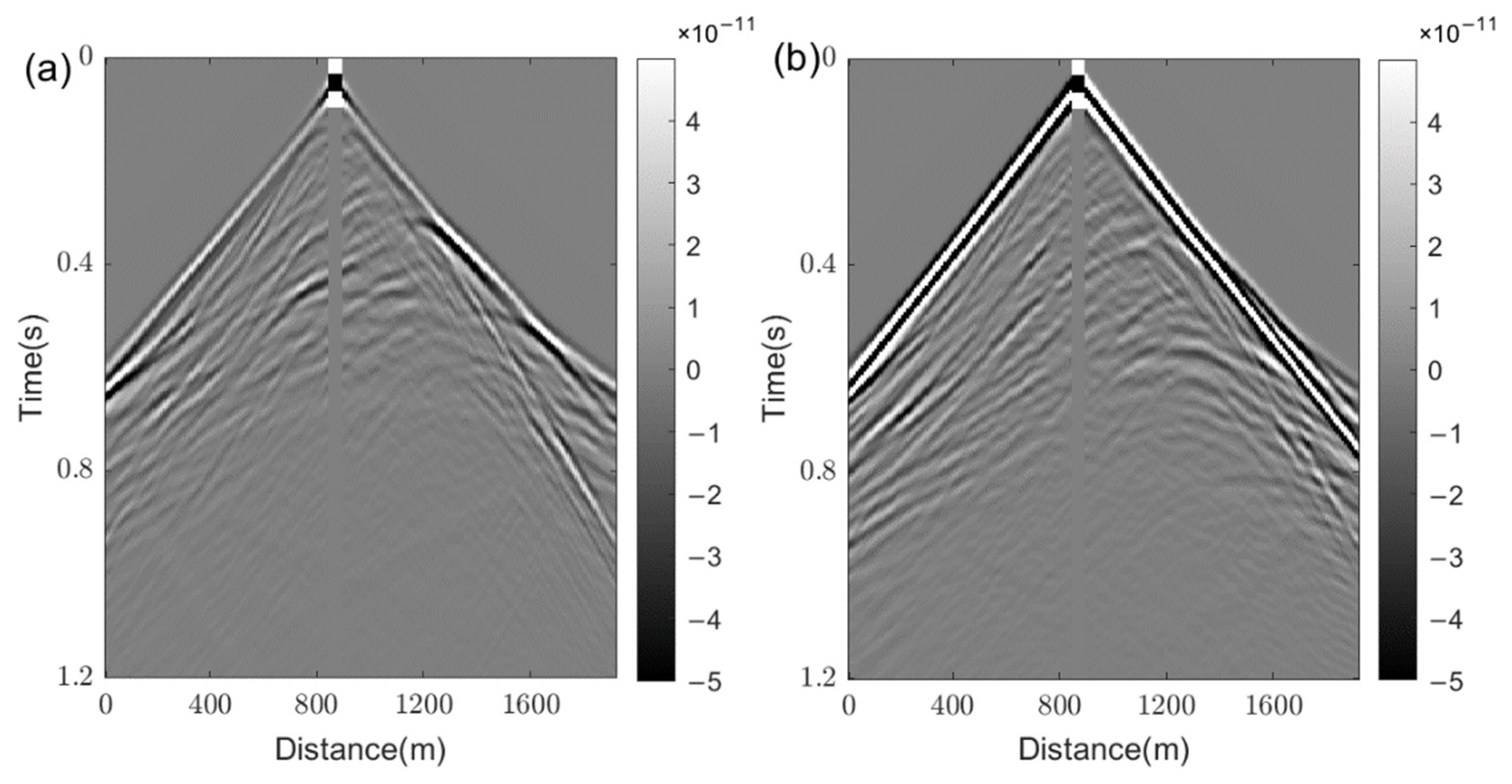
3.2. Inversion Effects Using Multi-Component Data with Bad Traces

In this section, we test the inversion effects using data with bad traces. In land seismic exploration, near-offset direct waves are often affected by surface waves, noise, acquisition conditions, and other factors. We used a sinusoidal function to generate bad traces near the source position to simulate these conditions. These bad traces were added to the near-offset position of each shot record. The multi-component observed seismic data of one shot are shown in Figure 9.

Now, we test the behavior of the objective functions of the L2EWI and CNEWI methods. The true velocity model and the initial velocity model are shown in Figure 2 and Figure 3, respectively. The true source wavelet is a Ricker wavelet with a dominant frequency of 20 Hz. A series of initial source wavelets was used to calculate the objective function value. The initial source wavelets were calculated by taking phase rotation of the true source wavelet with different degrees. The observed seismic data have near-offset bad traces, as described above. The behavior of the objective functions is shown in Figure 10. The convergence range of the CNEWI method is obviously wider than that of the L2EWI method. The minimum of the CNEWI objective function curve corresponds to the true source wavelet. However, the minimum of the L2EWI objective function curve does not correspond to the true solution, which demonstrates that the L2EWI method suffers the cycle-skipping problem and it is more sensitive to bad traces than the CNEWI method.

The L2EWI method and the CNEWI method were used to perform source wavelet inversion, and the results are shown in Figure 11. As a consequence of the presence of poor-quality traces, the L2EWI method fails to accurately determine both the amplitude and phase information of the source wavelet. In contrast, the CNEWI method demonstrates an improved accuracy in estimating the source wavelet. The obtained source wavelets were used to conduct elastic full-waveform inversion. Using multi-component seismic data, the elastic full-waveform inversion results are shown in Figure 12. Due to the obvious errors of the source wavelet in the L2EWI inversion, the inversion results in Figure 12a,b contain obvious velocity anomalies. The inversion results in Figure 12c,d show that both the P-wave and S-wave velocities are relatively close to the true velocity models, indicating that elastic full-waveform inversion based on CNEWI source wavelet estimation can still conduct robust inversion in the presence of bad traces. We extracted three traces from the inversion results in Figure 12, and the velocity comparison is shown in Figure 13. It can be seen that the proposed method can recover better absolute velocity values and velocity contrast information than the traditional method both for the P-wave velocity and the S-wave velocity.

3.3. Inversion Effects Using Single-Component Data with Bad Traces

In this section, we continue testing the inversion effects using data with bad traces, but assume that the data quality is poor and only single-component seismic data can be used for inversion. It is assumed that only X-component data are available. The observed data with bad traces were the same as the previous section, and one single-shot recording is shown in Figure 9b. The near-offset direct wave of the X-component observed data was intercepted to perform source wavelet inversion. The inversion results of the two methods are shown in Figure 14. It is evident that due to the influence of poor-quality traces, the L2EWI method has encountered challenges in achieving accurate source wavelet estimation results. There are obvious errors in the amplitude and phase information of the inverted source wavelet. The CNEWI method can still obtain good source wavelet estimation results, especially for the estimation of the phase information. Compared with the inversion results in Figure 12, we can see that using multi-component seismic data inversion can achieve better inversion results of the source wavelet. However, judging from the inversion results, for source wavelet inversion, whether single-component or multi-component seismic data are used, the CNEWI method can obtain reliable phase information of the source wavelet.

Still using the X-component seismic data, the source wavelets estimated by the L2EWI and CNEWI methods were used to conduct elastic full-waveform inversion, and the results are shown in Figure 15. It can be seen that due to obvious errors in the source wavelets estimated by the L2EWI method, there are obvious errors in the inversion results of Figure 15a,b. Elastic full-waveform inversion using source wavelets estimated by CNEWI shows robustness, and the inversion results in Figure 15c,d are significantly better than those in Figure 15a,b. However, since only the X-component data are used, the construction effect of the P-wave velocity model in Figure 15c is not as good as the S-wave velocity model in Figure 15d.

4. Conclusions

In this paper, we propose an elastic full-waveform inversion method based on CNEWI. The CNEWI method uses the normalized cross-correlation of near-offset direct waves to formulate an objective function, thereby mitigating the influence of inaccurate amplitudes or bad traces in seismic data during source wavelet inversion. Elastic full-waveform inversion based on CNEWI shows robustness in the presence of bad traces. Moreover, our proposed method addresses the noise and surface wave residuals commonly found in land seismic data, thereby improving the accuracy of both the source wavelet and velocity inversion processes. Incorporating multi-component seismic data enhances the precision of both source wavelet and velocity inversion. The numerical examples provided validate the robustness of our method in source wavelet inversion and the inversion of P-wave and S-wave velocities. The proposed method can provide relatively accurate source wavelet estimation in some complex cases, and also has good application potential for other cases that require high-accuracy source wavelet estimation, such as time-lapse seismic data processing.

References

1. Virieux, J.; Operto, S. An overview of full-waveform inversion in exploration geophysics. Geophysics 2009, 74, WCC1–WCC26. [Google Scholar] [CrossRef]
2. Bruno, P.P. Seismic Exploration Methods for Structural Studies and for Active Fault Characterization: A Review. Appl. Sci. 2023, 13, 9473. [Google Scholar] [CrossRef]
3. Tarantola, A. Linearized inversion of seismic reflection data. Geophys. Prospect. 1984, 32, 998–1015. [Google Scholar] [CrossRef]
4. Laily, P. The seismic inverse problem as a sequence of before-stack migrations. In Conference on Inverse Scattering—Theory and Application; SIAM: Philadelphia, PA, USA, 1983; pp. 206–220. [Google Scholar]
5. Tarantola, A. Inversion of seismic reflection data in the acoustic approximation. Geophysics 1984, 49, 1259–1266. [Google Scholar] [CrossRef]
6. Li, K.; Huang, X.; Hu, Y.; Chen, X.; Chen, K.; Tang, J. Vertical Seismic-Profile Data Local Full-Waveform Inversion Based on Marchenko Redatuming. Appl. Sci. 2023, 13, 4165. [Google Scholar] [CrossRef]
7. Plessix, R.E. A review of the adjoint-state method for computing the gradient of a functional with geophysical applications. Geophys. J. Int. 2006, 167, 495–503. [Google Scholar] [CrossRef]
8. Liu, F.; Morton, S.A.; Ma, X.; Checkles, S. Some key factors for the successful application of full-waveform inversion. Lead Edge 2013, 32, 1124–1129. [Google Scholar] [CrossRef]
9. Da Silva, S.L.; Costa, F.; Karsou, A.; Capuzzo, F.; Moreira, R.; Lopez, J.; Cetale, M. Research Note: Application of refraction full-waveform inversion of ocean bottom node data using a squared-slowness model parameterization. Geophys. Prospect. 2023; early view. [Google Scholar] [CrossRef]
10. Alaei, N.; Monfared, M.S.; Kahoo, A.R.; Bohlen, T. Seismic Imaging of Complex Velocity Structures by 2D Pseudo-Viscoelastic Time-Domain Full-Waveform Inversion. Appl. Sci. 2022, 12, 7741. [Google Scholar] [CrossRef]
11. Ishak, M.A.; Latiff, A.H.A.; Ho, E.T.W.; Fuad, M.I.A.; Tan, N.W.; Sajid, M.; Elsebakhi, E. Advanced Elastic and Reservoir Properties Prediction through Generative Adversarial Network. Appl. Sci. 2023, 13, 6311. [Google Scholar] [CrossRef]
12. Mora, P. Nonlinear two-dimensional elastic inversion of multioffset seismic data. Geophysics 1987, 52, 1211–1228. [Google Scholar] [CrossRef]
13. Rivera, C.; Trinh, P.; Bergounioux, E.; Duquet, B. Elastic multiparameter FWI in sharp contrast medium. In Proceedings of the 89th SEG Annual Meeting, San Antonio, TX, USA, 15–20 September 2019. [Google Scholar]
14. Tarantola, A. A strategy for nonlinear elastic inversion of seismic reflection data. Geophysics 1986, 51, 1893–1903. [Google Scholar] [CrossRef]
15. Crase, E.; Pica, A.; Noble, M.; McDonald, J.; Tarantola, A. Robust elastic nonlinear waveform inversion: Application to real data. Geophysics 1990, 55, 527–538. [Google Scholar] [CrossRef]
16. Basnet, M.B.; Anas, M.; Rizvi, Z.H.; Ali, A.H.; Zain, M.; Cascante, G.; Wuttke, F. Enhancement of In-Plane Seismic Full Waveform Inversion with CPU and GPU Parallelization. Appl. Sci. 2022, 12, 8844. [Google Scholar] [CrossRef]
17. Qin, N.; Liang, H.; Guo, Z.; Li, Z. A parallel implementing strategy for full waveform inversion of 3D elastic waves based on domain decomposition. Oil Geophys. Prospect. 2023, 58, 351–357. [Google Scholar]
18. Li, Q.; Wu, G.; Wang, Y.; Shen, G.; Duan, P. Elastic full-waveform inversion of land single-component seismic data based on optimal transport theory. Oil Geophys. Prospect. 2021, 56, 1060–1073. [Google Scholar]
19. Choi, Y.; Alkhalifah, T. Application of multi-source waveform inversion to marine streamer data using the global correlation norm. Geophys. Prospect. 2012, 60, 748–758. [Google Scholar] [CrossRef]
20. Zhang, Z.; Alkhalifah, T.; Wu, Z.; Liu, Y.; He, B.; Oh, J.-W. Normalized nonzero-lag crosscorrelation elastic full-waveform inversion. Geophysics 2019, 84, R1–R10. [Google Scholar] [CrossRef]
21. Shin, C.; Cha, Y.H. Waveform inversion in the Laplace domain. Geophys. J. Int. 2008, 173, 922–931. [Google Scholar] [CrossRef]
22. Wu, R.-S.; Luo, J.R.; Wu, B.Y. Seismic envelope inversion and modulation signal model. Geophysics 2014, 79, WA13–WA24. [Google Scholar] [CrossRef]
23. Luo, J.; Wu, R.-S.; Gao, J. Elastic seismic envelope inversion. J. Seism. Explor. 2016, 25, 103–119. [Google Scholar]
24. Chen, G.; Yang, W.; Liu, Y.; Wang, H.; Huang, X. Salt structure elastic full waveform inversion based on the multiscale signed envelope. IEEE Trans. Geosci. Remote Sens. 2022, 60, 4508912. [Google Scholar] [CrossRef]
25. Oh, J.-W.; Alkhalifah, T. Full waveform inversion using envelope-based global correlation norm. Geophys. J. Int. 2018, 213, 815–823. [Google Scholar] [CrossRef]
26. Zhang, P.; Han, L.; Yang, Y.; Shang, X. Source-independent cross-correlated elastic seismic envelope inversion for large-scale multiparameter reconstruction. IEEE Geosci. Remote Sens. Lett. 2022, 19, 8030305. [Google Scholar] [CrossRef]
27. Song, Z.-M.; Williamson, P.R.; Pratt, R.G. Frequency-domain acoustic-wave modeling and inversion of crosshole data: Part II—Inversion method, synthetic experiments and real-data results. Geophysics 1995, 60, 796–809. [Google Scholar] [CrossRef]
28. Pratt, R.G. Seismic waveform inversion in the frequency domain, Part 1: Theory and verification in a physical scale model. Geophysics 1999, 64, 888–901. [Google Scholar] [CrossRef]
29. Cheong, S.; Shin, C.; Pyun, S.; Min, D.J.; Suh, S. Efficient calculation of steepest descent direction for source-independent waveform inversion using normalized wavefield by convolution. In Proceedings of the 74th Annual International Meeting, SEG, Denver, CO, USA, 10–15 October 2004; pp. 1842–1845. [Google Scholar]
30. Choi, Y.; Shin, C.; Min, J.; Ha, Y. Efficient calculation of the steepest descent direction for source-independent seismic waveform inversion: An amplitude approach. J. Comput. Phys. 2005, 208, 455–468. [Google Scholar] [CrossRef]
31. Lee, K.H.; Kim, H.J. Source-independent full-waveform inversion of seismic data. Geophysics 2003, 68, 2010–2015. [Google Scholar] [CrossRef]
32. Zhou, B.; Greenhalgh, S.A. Crosshole seismic inversion with normalized full-waveform amplitude data. Geophysics 2003, 68, 1320–1330. [Google Scholar] [CrossRef]
33. Xu, K.; Greenhalgh, S.A.; Wang, M.Y. Comparison of source-independent methods of elastic waveform inversion. Geophysics 2006, 71, R91–R100. [Google Scholar] [CrossRef]
34. Choi, Y.; Min, D.J. Source-independent elastic waveform inversion using a logarithmic wavefield. J. Appl. Geophys. 2012, 76, 13–22. [Google Scholar] [CrossRef]
35. Choi, Y.; Alkhalifah, T. Source-independent time-domain waveform inversion using convolved wavefields: Application to the encoded multisource waveform inversion. Geophysics 2011, 76, R125–R134. [Google Scholar] [CrossRef]
36. Zhang, Q.C.; Zhou, H.; Li, Q.Q. Robust source-independent elastic full-waveform inversion in the time domain. Geophysics 2016, 81, R29–R44. [Google Scholar] [CrossRef]
37. Zhou, C.; Schuster, G.T.; Hassanzadeh, S.; Harris, J.M. Elastic wave equation traveltime and waveform inversion of crosswell data. Geophysics 1997, 62, 853–868. [Google Scholar] [CrossRef]
38. Hu, Y.; Han, L.; Xu, Z.; Zhang, T. Demodulation envelope multi-scale full waveform inversion based on precise seismic source function. Chin. J. Geophys. 2017, 60, 1088–1105. (In Chinese) [Google Scholar]
39. Shin, C.; Pyun, S.; Bednar, J.B. Comparison of waveform inversion, part 1: Conventional wavefield vs logarithmic wavefield. Geophys. Prospect. 2007, 55, 449–464. [Google Scholar] [CrossRef]
40. Kim, Y.; Min, D.-J.; Shin, C. Frequency-domain reverse-time migration with source estimation. Geophysics 2011, 76, S41–S49. [Google Scholar] [CrossRef]
41. Fang, Z.; Wang, R.; Herrmann, F. Source estimation for wavefield-reconstruction inversion. Geophysics 2018, 83, R345–R359. [Google Scholar] [CrossRef]
42. Zhang, P.; Han, L.; Lu, Z.; Shang, X.; Zhang, D. A Robust Source Wavelet Phase Inversion Method Based on Correlation Norm Waveform Inversion. IEEE Geosci. Remote Sens. Lett. 2023, 20, 7505405. [Google Scholar] [CrossRef]
43. Martin, G.S.; Wiley, R.; Marfurt, K.J. Marmousi2: An elastic upgrade for Marmousi. Lead Edge 2006, 25, 113–224. [Google Scholar] [CrossRef]
Figure 1. Cross-talk tests of the inversion algorithm. (a) and (b) are true P-wave and S-wave velocity models, respectively; (c) and (d) are initial P-wave and S-wave velocity models, respectively; (e) and (f) are inverted P-wave and S-wave velocity models, respectively.
Applsci 13 13014 g001
Figure 2. True velocity models. (a) True P-wave velocity model; (b) true S-wave velocity model.
Applsci 13 13014 g002
Figure 3. Initial velocity models. (a) Initial P-wave velocity model; (b) initial S-wave velocity model.
Applsci 13 13014 g003
Figure 4. Multi-component observed data. (a) Z-component observed data; (b) X-component observed data.
Applsci 13 13014 g004
Figure 5. Source wavelet inversion results in an ideal case.
Applsci 13 13014 g005
Figure 6. Direct wave comparison in an ideal case. (a) Z-component observed direct waves; (b) Z-component synthetic direct waves using an L2EWI-estimated source wavelet; (c) Z-component synthetic direct waves using a CNEWI-estimated source wavelet.
Applsci 13 13014 g006
Figure 7. Objective function curve comparison in an ideal case. (a) Objective function curves of the L2EWI process; (b) objective function curves of the CNEWI process.
Applsci 13 13014 g007
Figure 8. EFWI results comparison in an ideal case. (a) P-wave velocity model using source wavelet estimated by L2EWI; (b) S-wave velocity model using source wavelet estimated by L2EWI; (c) P-wave velocity model using source wavelet estimated by CNEWI; (d) S-wave velocity model using source wavelet estimated by CNEWI.
Applsci 13 13014 g008
Figure 9. Seismic data with bad traces. (a) Z-component seismic data with bad traces; (b) X-component seismic data with bad traces.
Applsci 13 13014 g009
Figure 10. Objective function behavior test in the case of existing bad traces.
Applsci 13 13014 g010
Figure 11. Source wavelet inversion results using multi-component seismic data with bad traces.
Applsci 13 13014 g011
Figure 12. EFWI results comparison using multi-component seismic data with bad traces. (a) P-wave velocity model using source wavelet estimated by L2EWI; (b) S-wave velocity model using source wavelet estimated by L2EWI; (c) P-wave velocity model using source wavelet estimated by CNEWI; (d) S-wave velocity model using source wavelet estimated by CNEWI.
Applsci 13 13014 g012
Figure 13. Extracted trace comparison of the inversion results in Figure 12. (a) P-wave velocity comparison; (b) S-wave velocity comparison. True: true velocity model; Initial: initial velocity model; L2EWI: inversion result by using the source wavelet estimated by L2EWI; CNEWI: inversion result by using the source wavelet estimated by CNEWI.
Applsci 13 13014 g013
Figure 14. Source wavelet inversion results using single-component seismic data.
Applsci 13 13014 g014
Figure 15. EFWI results comparison using single-component seismic data with bad traces. (a) P-wave velocity model using source wavelet estimated by L2EWI; (b) S-wave velocity model using source wavelet estimated by L2EWI; (c) P-wave velocity model using source wavelet estimated by CNEWI; (d) S-wave velocity model using source wavelet estimated by CNEWI.
Applsci 13 13014 g015
Disclaimer/Publisher’s Note: The statements, opinions and data contained in all publications are solely those of the individual author(s) and contributor(s) and not of MDPI and/or the editor(s). MDPI and/or the editor(s) disclaim responsibility for any injury to people or property resulting from any ideas, methods, instructions or products referred to in the content.