Novel Deep-Learning Approach for Automatic Diagnosis of Alzheimer’s Disease from MRI

Abstract

This study introduces a novel deep-learning methodology that is customized to automatically diagnose Alzheimer’s disease (AD) through the analysis of MRI datasets. The process of diagnosing AD via the visual examination of magnetic resonance imaging (MRI) presents considerable challenges. The visual diagnosis of mild to very mild stages of AD is challenging due to the MRI similarities observed between a brain that is aging normally and one that has AD. The detection of AD with extreme precision is critical during its early stages. Deep-learning techniques have recently been shown to be significantly more effective than human detection in identifying various stages of AD, enabling early-stage diagnosis. The aim of this research is to develop a deep-learning approach that utilizes pre-trained convolutional neural networks (CNNs) to accurately detect the severity levels of AD, particularly in situations where the quantity and quality of available datasets are limited. In this approach, the AD dataset is preprocessed via a refined image processing module prior to the training phase. The proposed method was compared to two well-known deep-learning algorithms (VGG16 and ResNet50) using four Kaggle AD datasets: one for the normal stage of the disease and three for the mild, very mild, and moderate stages, respectively. This allowed us to evaluate the effectiveness of the classification results. The three models were compared using six performance metrics. The results achieved with our approach indicate an overall detection accuracy of 99.3%, which is superior to the other existing models.

1. Introduction

Alzheimer’s disease (AD) is a degenerative neurological disorder that causes permanent brain cell loss and long-term cognitive impairment [1]. Alzheimer’s disease (AD) causes cognitive and mental deterioration, behavioral issues, language problems, and difficulty doing fundamental tasks. AD is a sixth-order death that destroys the brain area that controls breathing and cardiac function. There is no treatment to stop or slow the progression of Alzheimer’s disease [2], and its cause is unknown. Defects in the hippocampus, cerebral cortex, and ventricles are signs of Alzheimer’s disease. These areas control memory, planning, reasoning, and judgment [3]. Alzheimer’s disease (AD) progresses to varying degrees of severity. It is challenging to diagnose AD in its early and late stages because of MRI similarities between a normal aging brain and an AD brain. As a result, analyzing and assessing these pictures is challenging [4,5]. Until patients reach a moderate stage of AD, detection accuracy is low. Thus, it is crucial for AD diagnosis to detect changes in specific brain regions early on so that the disease can be halted in its tracks [6]. The ability of machine learning algorithms to detect AD has recently been demonstrated in studies [7,8]. MRI scans are frequently used in medical diagnoses. MRI scans may have varying meanings, depending on the reader. Supervised systems are trained using feature vectors extracted from medical imaging data. To extract these characteristics, human experts must expend significant time, resources, and energy. Rapid patient screening and diagnosis may be aided by deep-learning models. This technology can instantly analyze photographs without the need for skilled manual extraction. Features from MRI brain images are extracted using deep-learning-based methods, allowing for the early detection of AD. To mimic the performance of biological neural networks, scientists created ANNs [4,9]. Computers can learn from data at varying granularities due to their multi-layer processing architecture [10]. Deep learning is a subfield of machine learning (ML), which is a core component of artificial intelligence (AI). AI is used in many areas, including neuroscience. Predicting and diagnosing brain diseases, such as Alzheimer’s, has become much simpler thanks to AI. Deep learning has many types, such as the feed-forward deep neural network, the convolutional neural network (CNN), the auto-encoder (AE), the recurrent neural network (RNN), the deep belief network (DBN), and the generative adversarial network (GAN) [11].

CNN is a feed-forward neural network that makes use of convolutional features [12,13]. CNN, unlike other methods, does not require manual feature extraction. CNN kernels are analogous to various sensors that can respond to a wide variety of stimuli. Activation functions are similar to the way in which neurons send electric impulses to the next cell when a certain threshold is reached. CNN is better than most artificial neural networks in three ways: First, local connections are used between neurons in the same layer instead of between all neurons in the layer below; this lowers the parameters and speeds up convergence. Second, sharing the weight of links may reduce the total number of parameters if we combine link weights. Third, because convolution makes feature maps with a lot of features, the chance of overfitting goes up. Maximum and average pooling are two types of pooling that are recommended for reducing redundant work. The downsampling of dimensions: a pooling layer uses the idea of local correlation to downscale an image while preserving its essential details.

The following study demonstrates the efficacy of CNN in identifying AD. Ref. [14] proposed a CNN-Sparse Regression Network combination model for AD diagnosis. The model generated numerous representations at the target level using sparse regression networks. CNN was used to combine these representations at the target level to enhance output label recognition. A 16-layer VGGNet was used by the authors of reference [15] to effectively divide structural MRI scans into three groups: Alzheimer’s disease (AD), mild cognitive impairment (MCI), and normal cognitive (NC). The authors reported that segmentation was not conducted on the magnetic resonance (MR) images. Using functional MRI, ref. [16,17] applied the LeNet architecture to classify patients with Alzheimer’s disease from healthy controls. They came up with a technique for structural MRI that uses CNNs. The research demonstrated that CNN outperformed SVM. Future studies will likely include axial and sagittal MRI scans in addition to the standard coronal ones. The current result is 98.84% accurate, which is quite good. The use of structural MR images allowed for the development of a CNN-based AD diagnosis model [18]. Researchers found that by using both data augmentation and transfer learning together, overfitting could be lessened, and the models could use less computing power. Previous studies relied on smaller, regional datasets, but the authors of this one claim their work can be applied much more widely. In [19], an 8-layer CNN model was created specifically for AD diagnosis. To find the best model setup, the authors looked at many different activation function combinations, such as stochastic, max, and average pooling with ReLU, sigmoid, and leaky ReLU. A leaky ReLU activation function and a max pooling function were used in the most effective CNN models. A 3D-CNN model trained on MR images was proposed for AD diagnosis in [20]. They propose a 3D-CNN using the ResNet framework. Convolutional, dropout, pooling, and fully connected layers are some of the 36 it contains. The model outperformed expectations on a variety of performance metrics in experimental testing. Another method in [21] using 3D-CNN to examine MR images for AD signs was proposed. The authors deployed a Sobolev gradient optimizer, a leaky ReLU activation function, and a Max Pooling function. The three functions worked better together than separately. To aid in the diagnosis of AD, ref. [22] developed a 3D-FCNN-based model using MR images. The authors revealed that their proposed model outperformed several industry standards for both accuracy and robustness. The 3D-FCNN model outperformed the 2D-CNN on binary and multi-class classification tasks. An approach to diagnosing AD that uses structural MRI, genetic testing, and clinical evaluation was suggested in [23]. It is based on convolutional neural networks. The framework required fewer parameters than rivals like VGGNet and AlexNet for building CNN models. The method was quicker and less prone to overfitting in scenarios with sparse data. In [2], the authors propose using a CNN-based MR image model for the early detection of AD. The OASIS dataset, which is notoriously skewed, was used to train the model. To address the discrepancies present in the OASIS data set, data augmentation was implemented. According to the results of the experiments, the proposed model is superior to several state-of-the-art models.

A CNN-based MR image AD diagnosis model was proposed in [24]. It all started with voxelizing MR scans. Skull stripping was used to get rid of extra voxels, and the quality of the remaining ones was enhanced with a Gaussian filter. Independent component analysis was used to separate out different regions of the brain. In the end, the gray matter in the model was segmented. According to the results of the experiments, the proposed model is superior to other state-of-the-art models. The eight-layer CNN AD diagnosis model in [25] used drop-out regularization, data augmentation, and batch normalization to ensure excellent precision. The Siamese Convolutional Neural Network (SCNN) was introduced in [26] as a CNN-based model for dividing dementia into four distinct stages: moderate Alzheimer’s disease (MAD), mild dementia (MD), very mild dementia (VMD), and no dementia. Despite just having a small sample size to train on, the model’s results were reliable. The proposed model was shown to be superior to five other state-of-the-art studies. Ref. [27] proposed a cascaded 3D-CNN for AD diagnosis using structural MR images. To classify the input, the CNN model first retrieved features from it.

In order to diagnose Alzheimer’s disease using 3D-MR brain pictures, the authors in [28] modified V-Net to partition the bilateral hippocampus. They demonstrate the need for accurate hippocampi segmentation for an accurate AD diagnosis model. Compared to other segmentation and classification approaches, they state that the proposed design performed better. Ref. [29] developed a CNN model for AD diagnosis using MR images. To put the method to the test in real-world settings, the researchers looked at the correlation between relevance score and hippocampus volume. The 3D-CNN-SVM model for AD diagnosis was proposed in [30] based on MR images. It combines the 3D-CNN model to obtain features from MR images and SVM to classify the features. The 3D-CNN-SVM model provides a significant improvement over both 2D-CNN and classic 3D-CNN. Ref. [31] created a CNN using the DenseNet Bottleneck-Compressed architecture for the diagnosis of AD using MR images. The proposed model correctly classified the input 86% of the time. The EfficientNet models [32] are developed through the implementation of uncomplicated and exceptionally effective compound scaling methods. EfficientNet models demonstrate an enhanced level of precision and effectiveness in comparison to modern CNNs, including MobileNetV2, AlexNet, ImageNet, and GoogleNet [33]. EfficientNets show better accuracy through their compactness, computational efficiency, and generalization capabilities. Comparing eight different convolutional neural networks for early detection of Alzheimer’s disease, the EfficientNetB0 model has better evaluation metrics and needs fewer model parameters [34]. In a recent study [35], an EfficientNetB0 model was employed to diagnose AD. The results obtained for all performance metrics varied from 87% to 95%. The EfficientNetB0 model is very good at finding COVID-19 patterns in X-ray images while using a small amount of computing power compared to other popular architectures like ResNets and VGGs [36]. Subsequently, EfficientNets demonstrated high efficiency in numerous applications, including the detection of malaria parasites from blood smears and various COVID-19 detection applications [37]. Thus, the results of the EfficientNet series on different medical applications inspired us to develop an approach based on the EfficientNetB0 structure for AD.

This study introduces a comprehensive methodology for evaluating the severity and progression of Alzheimer’s disease (AD) from start to finish. Deep-learning techniques were utilized to distinguish between four stages of Alzheimer’s disease, specifically normal control, very mild, mild, and moderate dementia. This research endeavor aims to improve the performance of efficientNetB0 by implementing a three-step data processing approach. These steps involve the use of an alpha-trimmed filter for low-pass filtering, histogram equalization, and the application of transfer-learning techniques. In order to evaluate our approach performance, we compared it to two commonly utilized models, specifically ResNet50 and VGG16. The evaluation metrics employed for comparison encompassed precision, recall, accuracy, F1 score, confusion matrices, and receiver operating characteristic (ROC). In the following sections, the materials and methods are described. The results from experimental data, using datasets from official GitHub and Kaggle repositories, of three DL models are compared using six performance metrics. The proposed method was compared with two other well-performing deep-learning algorithms. Then, the results were discussed, conclusions drawn, and future directives were suggested.

2. Materials and Methods

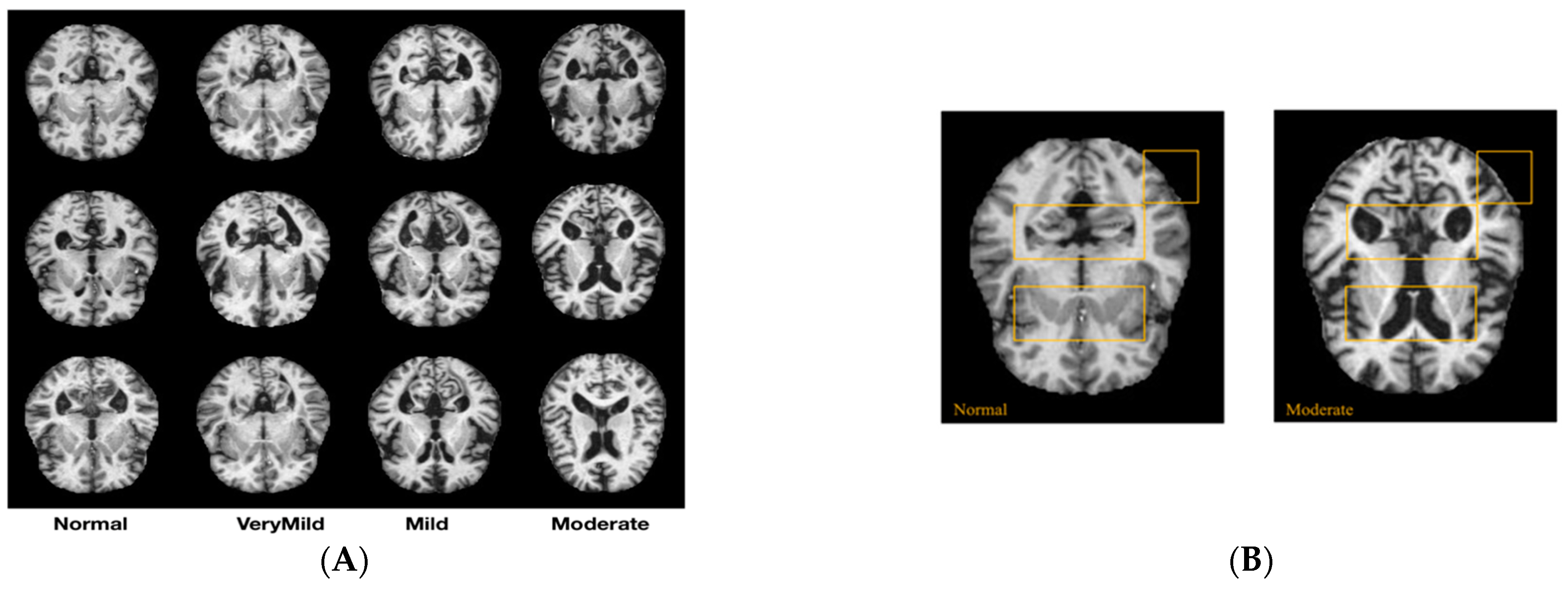
2.1. Dataset Description

The benchmark dataset research on the “Kaggle” website is available online: https://www.kaggle.com/datasets/tourist55/alzheimers-dataset-4-class-of-images (accessed on 11 February 2023). It provided MRI pictures of Alzheimer’s disease for this study [38]. Kaggle serves as a platform for providing online datasets for research and analysis in various fields. To expedite the development of enhanced algorithms for diagnosing and treating Alzheimer’s disease, we chose this dataset owing to its complete freedom, availability in diverse categories, and relatively small hard disk size, setting it apart from other popular datasets in the field. This manually collected dataset comprises MRI images verified and classified by Sarvesh Dubey [38]. Serving as valuable resources for training and testing deep-learning models with the objective of accurately predicting the stage of Alzheimer’s disease. By affording researchers and practitioners an opportunity to create algorithms for precise Alzheimer’s disease diagnosis, this dataset assumes a crucial role. Additionally, it contributes to the development of effective treatments. As the global burden of Alzheimer’s disease escalates, this dataset gains significance in advancing our understanding of the disease and improving patient outcomes [36].

A total of 6400 photos make up the Kaggle Alzheimer’s classification dataset (KACD). The dataset was divided into four groups: 896 mild AD, 64 moderate AD, 3200 normal, and 2240 very mild AD. To test the models, 20% of the dataset was used for testing, while 80% was used for training and analysis. The sample included 2560 normal controls, 717 participants with mild AD, 52 with moderate AD, and 1792 with very mild AD. A typical sample from each dataset class is shown in Figure 1. Doctors use the Hippocampal area as a biomarker to diagnose Alzheimer’s disease (AD) with great accuracy, making it a significant factor. However, hippocampus volume alone cannot predict early stages. According to prior study [4], cortical regions and thickness affect the illness’s progression. Due to its high resolution and contrast for soft tissues, structural MRI is used to evaluate the parietal, temporal, hippocampal, entorhinal cortex, and ventricular atrophy [6]. Different brain regions are modified depending on illness progression [4].

This study’s objective, as depicted in Figure 1, is to demonstrate how cognitive decline manifests differently in areas that have not experienced any disease and areas that have experienced the worst cases of the same disease [10]. In contrast to the moderate stage, individuals in the very mild and light stages of dementia exhibit a somewhat better level of independence in their functioning. However, due to notable memory impairment, they often require some level of support with various everyday activities. The severity stage is characterized by a prolonged duration compared to the very mild and mild stages. During this stage, the patient has a progressive deterioration of their physical condition, ultimately leading to mortality [39].

2.2. Proposed Method for AD Diagnosis

Figure 2 presents the general deep-learning workflow, where the first step is to choose the datasets for training and validation. Then, the selection of the hyper-parameters for the neural network model follows. In the third step, the choice of the CNN model and framework is determined by the related parameters, including the loss rate, learning function, and optimizer. The fourth step is the training and validation phase of the model. The fifth step is the testing and prediction phase using new input datasets. The final step is the assessment of the performance of the model.

Figure 3 presents the proposed approach for the classification of the AD images. The AD dataset is pre-processed first using pre-processing techniques, including skull removal and spatial registration, then another processing phase, including histogram equalization, slicing, and image resizing, followed by low-pass alpha-trimmed filtering. Skull removal is used to remove bones from the image. Histogram equalization is the normalization process of the gray levels in the images from various subjects and maps the pixel intensity values to a wide range.

In order to reduce the impact of orientation and spatial differences among scanner users, registration is performed. Registration improves the precision of the classification. The MNI152 brain template [40] was used by averaging 152 structural pictures into a single high-resolution image using non-linear registration. Slicing divides the image into multiple logical images. Resizing is carried out in order to get the desired image size (224 × 224).

Filtering improves the quality of the images by removing noise and artifacts. An alpha-trimmed filter was used to filter images from noise and artifacts. It first ranked the values of pixels in the neighbor window (5 × 5 pixels) centered on the pixel under processing. It ranks the pixels from the smallest to the biggest, eliminates the extremities according to the dimension of the parameter ‘d’ (Equation (1)), and then calculates the average of the remaining pixels. The resultant average will be placed at the same location (x,y) as the central pixel under processing in a new image.

The alpha-trimmed filter equation is

F(x,y) = (1/(mn − d))∑gr(s,t),

(1)

where

F(x,y): F represents the filtered image, and x,y are the coordinate of the pixel processed.

gr is the set of pixels left after excluding the d/2 extreme pixels.

mn is the dimensions of the filter.

d represents the number of pixels that will be excluded from the averaging.

(s,t) represents the set of coordinates of the remaining pixels.

In our implementation, the filter dimensions’ mn is 5 × 5, and d was set to 8. It means that we exclude 8 pixels out of 25, 4 from the beginning and 4 from the end of the ranked values of the pixels.

Then, the pre-processed data are fed as input to the DLS model using CNN model that performs feature extraction and classification of the input data. Finally, the model is evaluated using performance metrics such as F1 score, area under curve (AUC), recall, and precision.

Due to the small dataset, training big convolutional neural networks (CNNs) from the beginning proved difficult. Neural networks need a lot of data to train well, which may not be available. Instead of starting from scratch, using an existing model for a comparable job can save training time and improve outcomes [41]. CNN structure is presented in Figure 4.

As stated in reference [4], transfer learning facilitates accelerated training and compensates for the limited data set. It has been demonstrated that transfer learning is a dependable and effective initial method for developing interpretable deep-learning models. Transfer learning is an approach that applies pre-trained networks to novel tasks by modifying them, thereby efficiently classifying diverse datasets. Classifying medical images, such as brain MRI scans, with models initially trained on natural images from ImageNet [42] proves to be a particularly advantageous application. During training, this study utilizes pre-trained weights obtained from ImageNet [42]. Then, retraining networks on a new dataset through the modification of the final fully connected layers, except for the final fully connected layer, pre-trained layers are frozen, and each model is retrained using the dataset in this scenario. In order to generate class prediction probabilities, the output layer incorporates a fully connected layer with Softmax activation and a global pooling layer (Global Average Pooling).

The selection of ResNet50 and VGG16 for our research was predicated on their distinct attributes and benefits within the domain of medical image classification, specifically in the context of transfer-learning-based Alzheimer’s disease (AD) diagnosis. ResNet50 and VGG16 are pre-trained models, as described in [42]. By utilizing deep residual learning, ResNet50 overcomes the difficulty associated with training extremely deep networks. Additionally, ResNet50’s skip connection lets each layer make a link between its input and output, which makes it easier for the model to understand complicated features in medical images and speeds up the flow of data. The VGG16 architecture is selected due to its simple design, which incorporates deeper networks utilizing smaller convolutional filters (3 × 3). The simplicity of this approach facilitates the comprehension of acquired features, which is particularly critical in medical situations where it is vital to grasp the model’s reasoning process. Moreover, every layer in VGG16 represents a distinct level of abstraction, thereby establishing a distinct hierarchy of features. The hierarchical structure of this representation proves to be highly advantageous in the field of medical image analysis, wherein the significance of multiple levels of detail varies.

The configuration parameters for the three tested models are summarized in

Table 1. Summarize the hyper-parameters used for training.

Parameters	Proposed Method (PDL)	VGG16	ResNet50
Number of epochs	30	30	30
Batch Size	34	34	34
Optimiser	Adam	Adam	Adam
Learning Rate	0.0001	0.0001	0.0001
Loss Function	Categorical cross-entropy	Categorical cross-entropy	Categorical cross-entropy

. Under identical conditions, the objective of this configuration is to compare the F1 score, recall, and precision of these various neural network architectures. This guarantees that the hyperparameters for all three models are identical.

Throughout the experimental procedure, data preprocessing was conducted in a consistent manner for all models, thereby guaranteeing consistent data partitions for the purposes of training, validation, and testing as follows:

• For a consistent starting point, identical weights were assigned to each model during initialization.
• During training, the designated hyper-parameters were applied to the training set, while the progress of training was consistently monitored and assessed on the validation set.
• Using identical test set, performance metrics were computed for every model undergoing evaluation.
• To determine whether or not there were significant differences in performance metrics between models, statistical tests were employed, including ROC curve tests.

The results were graphically represented, incorporating precise recall curves or confusion matrices, which offered valuable insights into the merits and demerits of every model.

Proposed deep learning (PDL) is a CNN framework using EfficientNetB0, where architecture is presented in

Table 2. EfficientNetB0 architecture used in our model.

Steps	Operator	Resolution	Channels	Layers
1	Conv 3 × 3	224 × 224	32	1
2	MBconv1, 3 × 3	112 × 112	16	1
3	MBconv1, 3 × 3	112 × 112	24	2
4	MBconv1, 5 × 5	56 × 56	40	2
5	MBconv1, 3 × 3	28 × 28	80	3
6	MBconv1, 5 × 5	14 × 14	112	3
7	MBconv1, 5 × 5	14 × 14	192	4
8	MBconv1, 3 × 3	7 × 7	320	1
9	Conv 1 × 1 pooling	7 × 7	1280	1

, and a few other compounds explained in the next section. EfficientNetB0 has been purposefully engineered to attain competitive performance while minimizing computational demands. This characteristic renders it a highly suitable option for situations in which there are limitations on resources, such as those encountered in medical environments where computational resources may be limited, where EfficientNetB0 achieves a balance between model complexity and efficiency by uniformly scaling network dimensions. This is beneficial in the context of medical applications where optimizing resource utilization is a critical factor in achieving high predictive performance. EfficientNetB0 is famous for its efficiency and low cost. Due to compound scaling, the network’s depth, breadth, and resolution are equal. The EffifientNetB0 model was pre-trained using ImageNet, a large labeled dataset. Pre-trained weights from the ImageNet dataset were used during training. The transfer-learning technique was used to repair the pre-existing layers and then retrain the PDL model using Kaggle datasets.

PDL is composed of several blocks. Convolutional and pooling layers precede fully connected classification layers in each block. The PDL design included a batch normalizing layer before the fully connected layer, and a global average pooling (GAP) was used to build the model’s output layer. Layers were added after the fully connected layer flattened the model. The rectified linear unit (ReLU) activation function, global average pooling (GAP), 0.5 dropout layer, 4-unit dense layer, and Softmax activation function were used in these layers. After flattening the fully connected layer, one dense layer was applied; this layer was activated using ReLU, a dropout layer with a 0.5 dropout rate.

Mobile inverted residual bottleneck convolution (MBConv) [8] is a key characteristic used in several building blocks. Two pointwise convolution layers have a bottleneck layer. Pointwise convolutions increase output channels, while the bottleneck layer reduces input channels. To balance accuracy and performance, DLS uses compound scaling to customize its stack of MBConv layers. The compound scaling approach simultaneously modifies network depth, breadth, and resolution; this optimizes computing resources.

The DLS underwent training using an adaptive moment estimation (ADAM) optimizer, with a learning rate of 0.0001 and a batch size of 34. The training process consisted of a minimum of 20 epochs, during which a dropout rate of 0.5 was applied to the dropout layer.

In PDL, Softmax activation [43] was used to calculate class prediction probabilities using the dense function [44].

3. Results

The proposed method achieves its highest training and validation accuracy at epoch 20, reaching 99.8% and 99.0%, respectively. The corresponding losses for the training and validation sets are 0.006 and 0.02. The VGG16 architecture demonstrated lower performance in terms of training and validation accuracy at epoch 20, achieving rates of 99.4% and 98.2%, respectively. The corresponding losses were recorded as 0.025 and 0.05. In contrast, the ResNet50 network has a training accuracy of 98.0% and a validation accuracy of 96.5%, with corresponding loss values of 0.04 and 0.15. On the other hand, the proposed method has the advantage of requiring the least amount of time per iteration. Upon assessing the loss curve, it becomes apparent that the loss values of PDL exhibit a more rapid fall and tend towards zero in comparison to other networks. The VGG16 model has a higher iteration time compared to the PDL model, with the former taking around twice as long. On the other hand, the ResNet50 model demonstrates the longest training duration among the three models. All three models eventually converge; however, the PDL and VGG16 models have the fastest convergence rates.

The PDL model demonstrates a classification accuracy of over 98% and an error rate below 2% after five iterations. Both the ResNet50 and VGG16 models need more than 10 iterations. As a result, adversarial pictures only exhibit a minimal level of resilience. Consequently, the PDL and VGG16 models exhibit notable efficacy and robust convergence in the context of Alzheimer’s disease identification. Figure 5 presents the accuracy and loss metrics obtained from trained and validated databases over a span of 20 iterations using mixed data sets. Consequently, the PDL exhibits superior efficiency and accuracy in recognizing Alzheimer’s disease. The results prove that among the selected methods, the PDL has a notable capacity for generalization in Alzheimer’s disease recognition and is well suited for a broader range of diagnostic situations related to Alzheimer’s disease.

3.1. Prediction Performance

Figure 5 shows the accuracy and loss curves in the training and validation stages, where a blue line indicates training loss and a red line for validation loss indicates the three convolutional models we experimented with during this work, which were trained on four class datasets for 25 epochs.

Performance metrics are applied to test data by considering normal, very mild, mild, and moderate AD cases.

As shown in Figure 6, in terms of precision, recall, and F1 score, when comparing all methods, it is observed that PDL achieved the lowest loss value of 0.02 and performed the best accuracy of 99%. The lowest accuracy is obtained with ResNet50 (96.5%). For further in-depth evaluation of performance, the results are reported in

Table 3. Performance measures: comparison between pertained models architecture based on AD patients.

Models	Class Label	Precision (%)	Recall (%)	F1-Score (%)	Average Score
	Normal	98	97	98	97.6%
ResNet50	Very Mild	93	97	95	95%
	Mild	97	91	94	94%
	Moderate	100	100	100	100%
	Normal	98	99	99	98.6%
VGG16	Very Mild	98	97	97	97.3%
	Mild	100	98	99	99%
	Moderate	100	100	100	100%
	Normal	99	99	98	98.6%
Proposed Method	Very Mild	100	99	99	99.3%
	Mild	100	99	99	99.3%
	Moderate	100	100	100	100%

.

The prediction of the early stage of a very mild class is intriguing due to the inherent challenges associated with its diagnosis. In contrast, the classification of the late stage, which falls under the moderate category, is rather straightforward since all algorithms consistently yield a 100% accuracy rate in their results. In the early stages of AD, the PDL demonstrates superior performance with a precision of 100%, recall of 99%, and F1 score of 99%. In contrast, the ResNet50 and VGG16 models exhibit lower predictions, as shown in Table 3. Consequently, it is evident that PDL has superior performance in comparison to the other two models.

Additionally, in order to conduct a more comprehensive assessment of the classification models, Figure 7 presents a confusion matrix diagram that serves as a concise representation of the prediction outcomes during the evaluation of classification models on test data. The PDL model demonstrates remarkable performance in detecting both normal and early disease cases. In particular, the PDL yields 2–3% superior results compared to the VGG16 and ResNet50 models. It systematically summarizes the number of correctly or incorrectly predicted images. The vertical axis corresponds to the predicted class (output class), while the horizontal axis represents the true class (target class). Each confusion matrix is visually depicted as a heat map, utilizing color-coding techniques. The presence of darker pixels representing the diagonal elements is observable in all of the confusion matrices that have been displayed. This observation suggests that a substantial quantity of data is accurately classified in its corresponding category. In contrast, bright hues show instances of model misclassifications. The PDL achieved accurate classification for 1044 out of 1047 normal images, 698 out of 703 very mild images, and 269 out of 274 mild images. In contrast, it was shown that all algorithms exhibited accurate classification of the moderate AD group, while the very mild class demonstrated the lowest accuracy in classification. In the mild class, the VGG-16 model accurately predicted 267 out of the total mild images (274), whereas the ResNet-50 model properly identified 249 out of the total 274 AD images.

3.2. ROC Curves

The receiver operating characteristic (ROC) curve, which stands for “true positive rate vs. false positive rate”, is a graph that shows how well a classification model works with different types of classification criteria. The ROC curves, specifically the AUC (area under the ROC curve) values, for the proposed approach (PDL), VGG16, and ResNet50 models are compared in Figure 8 in relation to the four cases of Alzheimer’s disease. The ROC curves illustrate the individual AUC scores for each class as generated by three models, i.e., the classifiers that underwent training using EfficientNetB0 exhibited superior performance in comparison to those that were trained using ResNet50 and VGG16.

4. Discussion

This study tested transfer learning to train our proposed deep-learning algorithm with the objective of accurately classifying different stages of Alzheimer’s disease. This study compared our proposed method with two other well-known methods (VGG16 and ResNet50) on Kaggle AD datasets. The findings of our study exhibited a higher level of accuracy and yielded favorable results in comparison to other investigations [45]. The results of our work indicate that pre-trained models achieved high levels of accuracy without requiring data augmentation or extended training epochs. The utilization of hyper-parameters, as informed by previous research [46], involved the adjustment of batch size and learning rate to enhance the learning process and improve generalization accuracy. This enabled us to train CNNs that exhibit effective picture classification capabilities even when using less precise hyper-parameter values. Based on our results, it has been shown that a trained model has the ability to effectively classify AD into distinct phases with a high degree of accuracy. The classification results produced by the three distinct models are presented in Table 3, along with the corresponding values for four performance indicators. The proposed model demonstrated higher performance than VGG16 and Resnet50 for normal cases in terms of overall precision, with scores of 99.00%, 98.00%, and 98%, respectively. The evaluation of F1 score, precision, and recall performance metrics indicates that the proposed framework outperforms VGG16 in most scenarios. Equally, the ResNet50 model exhibits comparatively inferior performance outcomes compared to the other models. The consistency of the AUC values across all categories indicates that the predictions made by the proposed model are stable. Furthermore, the findings indicate that the prediction accuracy of both the VGG16 and ResNet50 models was comparatively lower for the mild and very mild stages. The results also indicated that the utilization of AD improved the ability to classify across all categories. A notable observation is that a significant proportion of the receiver operating characteristic (ROC) curves are situated above the linear reference line that connects the points (0,0) and (1,1). Nevertheless, the curves in question do not demonstrate a significant closeness to the upper-left corner, mostly because a restricted dataset was used for testing. Based on the confusion matrices depicted in Figure 7, it is apparent that the two highest-performing models exhibited nearly identical levels of accuracy when identifying MRI pictures associated with Alzheimer’s disease. The proposed model demonstrates accurate classification, with a success average rate of 98.6% for normal brain pictures and 99.3% for mild and very mild AD images. The VGG16-based model has an accuracy rate of 98.6% for correctly classifying normal cases, 99% for mild AD, and 97.3% for very mild AD images. The ResNet50 model demonstrates an accuracy rate of 97.3% for properly classifying normal brain images, 95% for accurately identifying very mild AD, and 94% for correctly classifying mild AD images. Based on the results of the analysis, it can be concluded that the performance of the proposed model surpassed that of the VGG16 and ResNet50 models for mild and very mild AD cases.

5. Conclusions

This paper describes an automated new method for diagnosing Alzheimer’s disease (AD) that uses image processing and novel deep transfer learning to figure out how bad the disease is and find important brain areas linked to it. The models use limited training sets of brain MRI scans. The empirical evaluations conducted in our study demonstrate that our proposed approach exhibited superior performance in handling the classification method compared to other popular state-of-the-art models. It attained an impressive overall average classification accuracy of 99.3%.

The findings of this work indicate that the proposed approach shows excellent performance in properly classifying Alzheimer’s disease (AD) and its various stages within a limited and restricted dataset. The findings underscore the capacity of computers to aid physicians in the process of diagnosing AD conditions. The proposed method demonstrated remarkable efficacy in extracting valuable information from pictures and accurately predicting prognostic indicators of the disease. Notably, this was achieved without requiring extensive image processing, optimization, or data augmentation techniques. Further research will be conducted to examine the impact of data augmentation techniques on the outcomes of various AD datasets.

References

1. Helaly, H.A.; Badawy, M.; Haikal, A.Y. Deep Learning Approach for Early Detection of Alzheimer’s Disease. Cogn. Comput. 2021, 14, 1711–1727. [Google Scholar] [CrossRef] [PubMed]
2. Islam, J.; Zhang, Y. Brain MRI Analysis for Alzheimer’s Disease Diagnosis Using an Ensemble System of Deep Convolutional Neural Networks. Brain Inform. 2018, 5, 2. [Google Scholar] [CrossRef] [PubMed]
3. Andrushia, A.D.; Sagayam, K.M.; Dang, H.; Pomplun, M.; Quach, L. Visual-Saliency-Based Abnormality Detection for MRI Brain Images—Alzheimer’s Disease Analysis. Appl. Sci. 2021, 11, 9199. [Google Scholar] [CrossRef]
4. Raju, M.; Thirupalani, M.; Vidhyabharathi, S.; Thilagavathi, S. Deep Learning Based Multilevel Classification of Alzheimer’s Disease Using MRI Scans. IOP Conf. Ser. Mater. Sci. Eng. 2021, 1084, 012017. [Google Scholar] [CrossRef]
5. Sethi, M.; Ahuja, S.; Rani, S.; Koundal, D.; Zaguia, A.; Enbeyle, W. An Exploration: Alzheimer’s Disease Classification Based on Convolutional Neural Network. BioMed Res. Int. 2022, 2022, 8739960. [Google Scholar] [CrossRef] [PubMed]
6. Pushpa, B.R.; Amal, P.S.; Kamal, N.P. Detection and stage wise classification of Alzheimer disease using deep learning methods. Int. J. Recent Technol. Eng. (IJRTE) 2019, 7, 206–212. [Google Scholar]
7. Sadat, S.U.; Shomee, H.H.; Awwal, A.; Amin, S.N.; Reza, T.; Parvez, M.Z. Alzheimer’s disease detection and classification using transfer learning technique and ensemble on Convolutional Neural Networks. In Proceedings of the 2021 IEEE Interna-tional Conference on Systems, Man, and Cybernetics (SMC), Melbourne, Australia, 17–20 October 2021. [Google Scholar] [CrossRef]
8. Vrahatis, A.G.; Skolariki, K.; Krokidis, M.G.; Lazaros, K.; Exarchos, T.P.; Vlamos, P. Revolutionizing the Early Detection of Alzheimer’s Disease through Non-Invasive Biomarkers: The Role of Artificial Intelligence and Deep Learning. Sensors 2023, 23, 4184. [Google Scholar] [CrossRef]
9. Lecun, Y.; Bengio, Y.; Hinton, G. Deep learning. Nature 2015, 521, 436–444. [Google Scholar] [CrossRef]
10. Danker, A.; Wirgård Wiklund, J. Using Transfer Learning to Classify Different Stages of Alzheimer’s Disease; KTH Royal INSTITUTE of Technology: Stockholm, Sweden, 2021; p. 33. [Google Scholar]
11. Saleem, T.J.; Zahra, S.R.; Wu, F.; Alwakeel, A.; Alwakeel, M.; Jeribi, F.; Hijji, M. Deep Learning-Based Diagnosis of Alzheimer’s Disease. J. Pers. Med. 2022, 12, 815. [Google Scholar] [CrossRef]
12. Saleem, T.J.; Chishti, M.A. Deep learning for Internet of Things data analytics. Procedia Comput. Sci. 2019, 163, 381–390. [Google Scholar] [CrossRef]
13. Suk, H.I.; Shen, D. Deep ensemble sparse regression network for Alzheimer’s disease diagnosis. In International Workshop on Machine Learning in Medical Imaging; Springer: Cham, Switzerland, 2016; pp. 113–121. [Google Scholar]
14. Billones, C.D.; Demetria, O.J.L.D.; Hostallero, D.E.D.; Naval, P.C. DemNet: A convolutional neural network for the detection of Alzheimer’s disease and mild cognitive impairment. In Proceedings of the 2016 IEEE Region 10 Conference (TENCON), Singapore, 22–25 November 2016; pp. 3724–3727. [Google Scholar]
15. Sarraf, S.; Tofighi, G. Classification of alzheimer’s disease using fmri data and deep learning convolutional neural networks. arXiv 2016, arXiv:1603.08631. [Google Scholar]
16. Sarraf, S.; Tofighi, G. Classification of Alzheimer’s disease structural MRI data by deep learning convolutional neural networks. arXiv 2016, arXiv:1607.06583. [Google Scholar]
17. Gunawardena, K.A.N.N.P.; Rajapakse, R.N.; Kodikara, N.D. Applying convolutional neural networks for pre-detection of alzheimer’s disease from structural MRI data. In Proceedings of the 2017 24th International Conference on Mechatronics and Machine Vision in Practice (M2VIP), Auckland, New Zealand, 21–23 November 2017; pp. 1–7. [Google Scholar]
18. Basaia, S.; Agosta, F.; Wagner, L.; Canu, E.; Magnani, G.; Santangelo, R.; Filippi, M.; Alzheimer’s Disease Neuroimaging Initiative. Automated classification of Alzheimer’s disease and mild cognitive impairment using a single MRI and deep neural networks. NeuroImage Clin. 2019, 21, 101645. [Google Scholar] [CrossRef] [PubMed]
19. Wang, S.-H.; Phillips, P.; Sui, Y.; Liu, B.; Yang, M.; Cheng, H. Classification of Alzheimer’s disease based on eight-layer convolutional neural network with leaky rectified linear unit and max pooling. J. Med. Syst. 2018, 42, 85. [Google Scholar] [CrossRef]
20. Karasawa, H.; Liu, C.-L.; Ohwada, H. Deep 3d convolutional neural network architectures for alzheimer’s disease diagnosis. In Asian Conference on Intelligent Information and Database Systems; Springer: Cham, Switzerland, 2018; pp. 287–296. [Google Scholar]
21. Goceri, E. Diagnosis of Alzheimer’s disease with Sobolev gradient-based optimization and 3D convolutional neural network. Int. J. Numer. Methods Biomed. Eng. 2019, 35, e3225. [Google Scholar] [CrossRef]
22. Tang, H.; Yao, E.; Tan, G.; Guo, X. A fast and accurate 3D fine-tuning convolutional neural network for Alzheimer’s disease diagnosis. In International CCF Conference on Artificial Intelligence; Springer: Singapore, 2018; pp. 115–126. [Google Scholar]
23. Spasov, S.E.; Passamonti, L.; Duggento, A.; Liò, P.; Toschi, N. A multi-modal convolutional neural network framework for the prediction of Alzheimer’s disease. In Proceedings of the 2018 40th Annual International Conference of the IEEE Engineering in Medicine and Biology Society (EMBC), Honolulu, HI, USA, 18–21 July 2018; pp. 1271–1274. [Google Scholar]
24. Basheera, S.; Ram, M.S.S. Convolution neural network–based Alzheimer’s disease classification using hybrid enhanced independent component analysis based segmented gray matter of T2 weighted magnetic resonance imaging with clinical valuation. Alzheimer’s Dement. Transl. Res. Clin. Interv. 2019, 5, 974–986. [Google Scholar] [CrossRef]
25. Jiang, X.; Chang, L.; Zhang, Y.-D. Classification of Alzheimer’s disease via eight-layer convolutional neural network with batch normalization and dropout techniques. J. Med. Imaging Health Inform. 2020, 10, 1040–1048. [Google Scholar] [CrossRef]
26. Mehmood, A.; Maqsood, M.; Bashir, M.; Shuyuan, Y. A deep siamese convolution neural network for multi-class classification of alzheimer disease. Brain Sci. 2020, 10, 84. [Google Scholar] [CrossRef]
27. Raju, M.; Gopi, V.P.; Anitha, V.S.; Wahid, K.A. Multi-class diagnosis of Alzheimer’s disease using cascaded three dimensional convolutional neural network. Phys. Eng. Sci. Med. 2020, 43, 1219–1228. [Google Scholar] [CrossRef]
28. Sun, J.; Yan, S.; Song, C.; Han, B. Dual-functional neural network for bilateral hippocampi segmentation and diagnosis of Alzheimer’s disease. Int. J. Comput. Assist. Radiol. Surg. 2020, 15, 445–455. [Google Scholar] [CrossRef]
29. Dyrba, M.; Hanzig, M.; Altenstein, S.; Bader, S.; Ballarini, T.; Brosseron, F.; Buerger, K.; Cantré, D.; Dechent, P.; Dobisch, L.; et al. Improving 3D convolutional neural network comprehensibility via interactive visualization of relevance maps: Evaluation in Alzheimer’s disease. arXiv 2020, arXiv:2012.10294. [Google Scholar] [CrossRef] [PubMed]
30. Feng, W.; Halm-Lutterodt, N.V.; Tang, H.; Mecum, A.; Mesregah, M.K.; Ma, Y.; Li, H.; Zhang, F.; Wu, Z.; Yao, E.; et al. Automated MRI-based deep learning model for detection of Alzheimer’s disease process. Int. J. Neural Syst. 2020, 30, 2050032. [Google Scholar] [CrossRef] [PubMed]
31. Solano-Rojas, B.; Villalón-Fonseca, R. A Low-Cost Three-Dimensional DenseNet Neural Network for Alzheimer’s Disease Early Discovery. Sensors 2021, 21, 1302. [Google Scholar] [CrossRef] [PubMed]
32. Tan, M.; Le, Q.V. EfficientNet: Rethinking Model Scaling for Convolutional Neural Networks. In Proceedings of the 36th International Conference on Machine Learning, Long Beach, CA, USA, 10–15 June 2019. [Google Scholar]
33. Marques, G.; Agarwal, D.; de la Torre Díez, I. Automated medical diagnosis of COVID-19 through EfficientNet convolutional neural network. Appl. Soft Comput. 2020, 96, 106691. [Google Scholar] [CrossRef] [PubMed]
34. Agarwal, D.; Berbis, M.A.; Martín-Noguerol, T.; Luna, A.; Garcia, S.C.P.; de la Torre-Díez, I. End-to-end deep learning architectures using 3D neuroimaging biomarkers for early Alzheimer’s diagnosis. Mathematics 2022, 10, 2575. [Google Scholar] [CrossRef]
35. Agarwal, D.; Berbís, M.Á.; Luna, A.; Lipari, V.; Ballester, J.B.; de la Torre-Díez, I. Automated Medical Diagnosis of Alzheimer’s Disease Using an Efficient Net Convolutional Neural Network. J. Med. Syst. 2023, 47, 57. [Google Scholar] [CrossRef] [PubMed]
36. Luz, E.; Silva, P.L.; Silva, R.; Silva, L.; Guimarães, J.; Miozzo, G.; Moreira, G.; Menotti, D. Towards an effective and efficient deep learning model for COVID-19 patterns detection in X-ray images. arXiv 2021, arXiv:2004.05717. [Google Scholar] [CrossRef]
37. Zebin, T.; Rezvy, S. COVID-19 Detection and Disease Progression Visualization: Deep Learning on Chest X-rays for Classification and Coarse Localization. Appl. Intell. 2021, 51, 1010–1021. [Google Scholar] [CrossRef]
38. Dubey, S. Alzheimer’s Dataset (4 Class of Images). Available online: https://www.kaggle.com/tourist55/alzheimers-dataset-4-class-of-images (accessed on 29 November 2020).
39. Fu’adah, Y.N.; Wijayanto, I.; Pratiwi, N.K.C.; Taliningsih, F.F.; Rizal, S.; Pramudito, M.A. Automated Classification of Alzheimer’s Disease Based on MRI Image Processing Using Convolutional Neural Network (CNN) With AlexNet Architecture. J. Physics Conf. Ser. 2021, 1844, 012020. [Google Scholar] [CrossRef]
40. Atlases—NIST. Available online: https://nist.mni.mcgill.ca/atlases/ (accessed on 20 March 2023).
41. Kang, H.; Park, H.-M.; Ahn, Y.; Van Messem, A.; De Neve, W. Towards a Quantitative Analysis of Class Activation Mapping for Deep Learning-Based Computer-Aided Diagnosis. In Proceedings of the Medical Imaging 2021: Image Perception, Observer Performance, and Technology Assessment, Online, 15–19 February 2021; Samuelson, F.W., Taylor-Phillips, S., Eds.; SPIE: Bellingham, WA, USA, 2021; Volume 11599. [Google Scholar] [CrossRef]
42. Lim, B.Y.; Lai, K.W.; Haiskin, K.; Kulathilake, K.A.S.H.; Ong, Z.C.; Hum, Y.C.; Dhanalakshmi, S.; Wu, X.; Zuo, X. Deep Learning Model for Prediction of Progressive Mild Cognitive Impairment to Alzheimer’s Disease Using Structural MRI. Front. Aging Neurosci. 2022, 14, 876202. [Google Scholar] [CrossRef]
43. Kabani, A.; El-Sakka, M.R. Object Detection and Localization Using Deep Convolutional Networks with Softmax Activation and Multi-class Log Loss. In Proceedings of the 2016 International Conference on Image Analysis and Recognition (ICIAR 2016), Póvoa de Varzim, Portugal, 13–15 July 2016; pp. 358–366. [Google Scholar]
44. Deng, J.; Dong, W.; Socher, R.; Li, L.-J.; Li, K.; Fei-Fei, L. ImageNet: A large-scale hierarchical image database. In Proceedings of the 2009 IEEE Conference on Computer Vision and Pattern Recognition, Miami, FL, USA, 20–25 June 2009; pp. 248–255. [Google Scholar] [CrossRef]
45. Prakash, D.; Madusanka, N.; Bhattacharjee, S.; Park, H.-G.; Kim, C.-H.; Choi, H.-K. A Comparative Study of Alzheimer’s Disease Classification using Multiple Transfer Learning Models. J. Multimedia Inf. Syst. 2019, 6, 209–216. [Google Scholar] [CrossRef]
46. Kandel, I.; Castelli, M. The Effect of Batch Size on the Generalizability of the Convolutional Neural Networks on a Histopathology Dataset. ICT Express 2020, 6, 312–315. [Google Scholar] [CrossRef]
Figure 1. (A) Magnetic resonance imaging (MRI) images (2D) from the KACD dataset with four of Alzheimer’s dementia’s stages. (B) The images highlight major regions of healthy brain (left) and an Alzheimer’s brain (right), as indicated in yellow.
Applsci 13 13051 g001
Figure 2. Deep-learning workflow.
Applsci 13 13051 g002
Figure 3. Proposed DL (PDL)-based classification approach.
Applsci 13 13051 g003
Figure 4. CNN architecture.
Applsci 13 13051 g004
Figure 5. The accuracy and loss curves in the training and validation stages for the 3 models; blue lines represent training, and red lines represent validation. The first raw images, from the top, represent the accuracy and loss of Resnet50; the second raw images represent the accuracy and loss of VGG16; and the third raw images represent the accuracy and loss of PDL.
Applsci 13 13051 g005aApplsci 13 13051 g005b
Figure 6. (A) The performance metric of F1 score, where ResNet50 results are shown in blue, VGG16 results are shown in yellow, and PDL results are shown in green. (B) The performance metric of precision, where ResNet50 results are shown in blue, VGG16 results are shown in yellow, and PDL results are shown in green. (C) The performance metric of recall, where ResNet50 results are shown in blue, VGG16 results are shown in yellow, and PDL results are shown in green.
Applsci 13 13051 g006
Figure 7. The confusion matrices of ResNet50, VGG16, and PDL are presented in (AC), respectively. The dark blue square represents normal (non-AD), the sky blue represents very mild, the gray represents mild, and the non-colored square represents moderate. The horizontal axis represents the predicted label, and the vertical axis represents the true label. The number in the center of each square represents the number of images that were classified correctly. The other numbers represent the misclassification.
Applsci 13 13051 g007aApplsci 13 13051 g007b
Figure 8. Representing the ROC curves, the vertical axis represents the true positive rate, and the horizontal axis represents the false positive rate. It shows the class-wise AUC scores obtained by the three models: (A) represents the proposed method; (B) represents VGG16; and (C) represents ResNet50. Blue represents the normal case (class 1), orange represents very mild AD (class 2), green represents mild AD (class 3), and red represents moderate AD (class 4).
Applsci 13 13051 g008