Article

Design and Characterization of a Single Lever Bicycle Brake with Hydraulic Pressure Proportioning

by
Michael D. Machado
and
Vimal K. Viswanathan
*
Department of Mechanical Engineering, San Jose State University, San Jose, CA 95112, USA
*
Author to whom correspondence should be addressed.
Appl. Sci. 2023, 13(3), 1767; https://doi.org/10.3390/app13031767
Submission received: 4 January 2023 / Revised: 26 January 2023 / Accepted: 26 January 2023 / Published: 30 January 2023
(This article belongs to the Section Mechanical Engineering)

Abstract

:

Featured Application

The work described here aims to design and characterize a more efficient bicycle braking system.

Abstract

In 2019, the Centers for Disease Control and Prevention estimated that 329,000 Americans were injured in cycling-related incidents. Since the first bicycle brake in 1817, there has been an individual brake lever for decelerating each wheel, while on cars, there has been a single control lever for decelerating multiple wheels since 1921. To perform an emergency stop on a bicycle, the rider must proportion hand pressure on each brake lever and simultaneously vary hand pressure throughout the duration of the maneuver to match the variations of normal force on each tire. Only highly skilled riders, with years of training and practice, can correctly proportion brake pressure to maximize available traction and thus minimize stopping distances. The objective of this study is to simulate and prototype a hydraulic, single-lever bicycle brake system, integrating front and rear brake proportioning, which minimizes stopping distance compared to dual-lever simulations. A design is developed to address the brake proportioning issue. Based on the simulations and physical model, the prototype proportioning valve decreased simulated stopping distances up to 18%. Exploring a range of bike types and scenarios, stopping distances were decreased between 13% and 26%. Simulating an ideal proportioning valve, stopping distances were further decreased between 4% and 40%. These results show that there can be an advantage to brake proportioning technologies in bicycles.

1. Introduction

Since the first bicycle brake in 1817, there has been an individual brake lever for decelerating each wheel [1], while on cars, there has been a single control lever for decelerating multiple wheels since 1921 [2]. To perform an emergency stop on a bicycle, the rider must proportion hand pressure on each brake lever and simultaneously vary hand pressure throughout the duration of the maneuver to match the variations of normal force on each tire [3]. Only highly skilled riders, with years of training and practice, can correctly proportion brake pressure to maximize available traction and thus minimize stopping distances.
In 2019, the Centers for Disease Control and Prevention estimated that 329,000 Americans were injured in cycling-related incidents [4]. If a system that simplifies the braking process and decreases stopping distances can prevent a small fraction of these injuries, then a large impact on bicycle safety can be made. Worldwide e-bike (electronic bicycle) sales have been growing exponentially since 2006, with the majority of the growth coming from the European and United States markets [5]. Furthermore, e-bike sales in the United States more than doubled between 2019 and 2020, with sales volumes soaring from 270,000 to 600,000 units [6].
Due to the higher speed and mass of e-bikes, the required stopping distances can be much greater than a non-assist pedal bike, likely leading to numerous and significant injuries. E-bikes are particularly suited for brake proportioning technologies because they are not only faster and heavier but also have a lower center of mass, hydraulic disc brakes, and regenerative braking.

1.1. How Riders Proportion Hand Force on Each Brake Lever

A study involving six participants riding e-bikes for a total of 32.5 h in a natural setting recorded 1566 braking events. On average, for routine braking, both levers were used during 11.7% of the braking events, with that figure increasing to 43.5% for unexpected braking events, with four out of six riders preferring to use the rear brake only. The peak deceleration rates averaged over all six participants was 1.56 ± 0.69 m/s2 [7]. This is below the theoretical maximum deceleration before tip-over (where the rider is ejected over the front wheel due to excessive deceleration), which is formulated in Equation (5) and shown to be in the range of 6.7 m/s2 to 7.4 m/s2 for e-bikes. Although this is not a statistically significant sample size, these riders could greatly decrease stopping distances by utilizing more front braking force.

1.2. Numerical Analysis of Longitudinal Bicycle Braking Dynamics

A bicycle with a 40% front and 60% rear weight distribution, 1.067 m wheelbase, and 1.1 m center of gravity height decelerating at 4.91 m/s2, can only apply 10% of the total braking force to the rear wheel before lockup occurs. More than twice the braking distance is required with rear-only braking as compared to front-only braking, further magnifying the issues with rear-only braking [3]. Closed-form solutions exist to predict the stopping distance for different brake balances, which account for friction coefficients, road gradients, bicycle parameters, rider parameters, inertia, aerodynamic drag, and reaction times [8]. A multibody simulation using five bodies and three revolute joints, was used to evaluate the effectiveness of preventing tip-over through seat post-actuation, fork anti-dive control, and front brake pressure control, with results illustrating the regions of tip-over potential [9]. A multibody simulation is advantageous when investigating the specific mechanism of tip-over, but the extra level of complexity may be unnecessary for modeling bicycles with a rigid frame.

1.3. Numerical Analysis of Hydraulic Bicycle Brake Systems

Research demonstrates that multi-domain physical simulation software can be used to simulate hydraulic brake systems and run test bench hardware with hydraulic pressure sensors to collect results. As the system pressure increases, brake torque increases at a non-linear rate due to a drop in brake pad to rotor friction coefficient experienced at higher pressures. However, as the rotor temperature increases, this friction coefficient also increases [10]. Additionally, a bicycle can be instrumented with brake pressure, wheel speed, longitudinal acceleration, and vertical position sensors, then ridden in a natural environment. The numerical information gathered from these sensors can be used to develop a braking control algorithm [11]. Having an accurate simulation of the braking system is essential for modeling the entire braking process.

1.4. Using Haptic Feedback to Regulate Brake Lever Force

Brake pressure modulation and proportioning can be achieved by providing haptic feedback for the rider in the form of an oscillating offset weight on the brake lever which vibrates when the rider reaches a preset deceleration rate. Results from testing with haptic feedback set at 3 m/s2 up to 6 m/s2 show that a rider sensing the vibration can modulate their deceleration rates, which decreases their time spent in the tip-over deceleration region for all tests [12]. A patent filed by the authors details the sensors, vibratory actuators, and control software needed to communicate the braking limit to the rider [13]. When used by experienced riders, a haptic feedback system could decrease stopping distances. Haptic feedback could also be used to train novice riders on the proper proportioning ratio of front-to-rear brake application force.

1.5. Anti-Lock Braking Systems for Bicycles

A mechanism mimicking motor vehicle anti-lock braking systems was implemented using the braking force to supply power to the system, thus relying on very little electrical power; however, this also required a bulky attachment and redesign of the brake mount interface [14]. Utilizing an electrostatic hydraulic actuator weighing only 270 g, not including the battery, a lower mass solution for bicycles was prototyped and tested. This system relies only on the actuator, encoder, and control unit. Results from tests and simulations using wheel deceleration and actuator position as the only necessary control inputs showed promising results using a proportional-integral controller [15]. This study did not consider corrections for longitudinal fork deflections, which another study demonstrated numerically and experimentally to result in around 10% slip angle error [16].

1.6. Braking Torque Applied during Bicycle Battery Regeneration

Testing on brushless DC motors shows a max regenerative torque of 13 N·m at 50 rev/min (100% load), resulting in 11 W of braking power. This provides a correlation of torque and angular velocity down to 0% load [17]. Another study provides a closed-form solution for stopping power based on specific voltage and current measurements but also outlines a control algorithm where regeneration power is based on a rider’s desired braking torque [18]. It may be important to have the torque provided by regenerative braking accounted for when deciding front and rear brake proportioning.

1.7. Aerodynamic Drag as a Factor in Deceleration

Aerodynamic drag is an important factor in bicycle braking because aerodynamic power dissipation is a factor of velocity cubed. At 10 m/s, aerodynamic drag can provide over 400 W of power dissipation for an upright cyclist with a drag coefficient of 1.15 and a frontal area of 0.55 m2 [3]. The frontal area can be calculated using pixel measurements of photos. Using this technique with 17 cyclists with an average height of 1.76 ± 0.08 m and body mass of 68.3 ± 9.2 kg, it was found that, in the upright position, their frontal area was 0.605 ± 0.069 m2 [19]. These values are required for developing an accurate braking simulation.

1.8. Industry Standards

Both the CPSC (Consumer Product Safety Commission) and ISO (International Organization for Standardization) have outlined regulations concerning bicycle brakes. These standards define both the design criteria and testing requirements that must be met by bicycle braking systems. The CPSC allows for a single lever to control both front and rear calipers [20]; however, the ISO mandates “at least two independently actuated braking systems” [21]. Applying the corrections mentioned in the standards leads to the test specifications shown in Table 1.
The objective of this study is to simulate and prototype a hydraulic, single-lever bicycle brake system, integrating front and rear brake proportioning, which minimizes stopping distance compared to dual-lever simulations. The simulated stopping distance will be corroborated with independent, external field test results. The simulated front and rear brake caliper force as a function of lever force will be validated with sensor data from the stand-alone prototype.
This paper will start by describing the method of physical prototype and simulation model development, then describe the corroboration of the simulation model with theoretical formulations and empirical testing. Next, the physical prototype will be described along with the results of prototype testing, then investigations into the critical regions of brake proportioning will be conducted. Lastly, the prototype data results will be integrated into the simulation model and various longitudinal braking scenarios, including the different center of mass positions and road gradients, will be analyzed.

2. Method

The initial step was to develop the bicycle braking simulation in Simulink. The next step was to ensure corroboration between the simulation and the derived equations of motion. This was further corroborated by comparison to external, independent test results of a bicycle performing an emergency stop. The next phase was ideation which culminated in concept selection. Concurrently, a prototype single-lever system with lever force, caliper force, and system pressure sensors were built without proportioning. This initial prototype was used to test the sensor setup and characterize the lever-to-caliper force ratio. Commercially available, adjustable proportioning valves were tested for suitability with a bicycle brake system. A CAD model of the proportioning device was then created in SOLIDWORKS. Next, experiments were run on the prototype and the braking simulation was updated with the experimental caliper-to-lever force relationship.
As illustrated in Figure 1, force sensors measure the applied force on the lever and the clamping force of both brake calipers. A pressure transducer measured the hydraulic line pressure and was calibrated against a pressure gauge with ±2% accuracy. All three force sensors were calibrated with known weights. The data acquisition equipment wiring diagrams and program code for the test layout shown in Figure 1 is provided in the Supplementary Materials.
The experiment began by applying and measuring a continuously increasing load at the brake lever. The line pressure, along with the front and rear caliper clamping force, were measured during the lever load application. The level of pressure proportioning between each caliper was varied between runs, and multiple runs were conducted for each setting.

3. Results

3.1. Theoretical Stopping Distance Calculation

The theoretical minimum stopping distance from Wilson and Schmidt’s book (Equation (1)) calculates stopping distance as a function of three variables, velocity (v), tire coefficient of friction (μ), and gravitational acceleration (g), while only neglecting air drag, rolling resistance, and tip-over [3].
S = v 2 2 μ g
Adding air drag, rolling resistance, and separate front and rear braking parameters to a closed-form braking calculation in MATLAB, Lieh provides a more thorough analytical representation of braking maneuvers and allows for the comparison of different front and rear brake proportioning values [22]. Using MathWorks software, Maier et al. developed a 13 D.O.F. numerical model and simulated the maximum deceleration before tip-over for different rider parameters [23].
Empirical testing was performed by Klug et al. on an electric bicycle with front and rear wheel speed sensors. A series of stops were performed from an initial velocity of 20 km/h with equal front and rear brake pressure, controlled by a limit stop on the handlebars and increased until the rear wheel lock occurred [9]. Bicycle deceleration performance was field tested by Famiglietti et al. on a variety of bicycles instrumented with accelerometers. Stopping distance was measured with a synchronized video, but only mass, wheelbase length, initial velocity, and acceleration were given for each test [24].

3.2. Longitudinal Braking Model of a Bicycle

The Simulink Vehicle Dynamics Toolbox was used to represent the longitudinal deceleration of a bicycle. This model uses a single degree of freedom longitudinal vehicle dynamics block and two longitudinal wheel blocks. The longitudinal dynamics block uses grade angle, wind speed, and longitudinal tire forces as inputs and outputs velocity and normal axle force. These are fed to the tire blocks, which output wheel rotational velocities and longitudinal tire forces. The single degree of freedom longitudinal dynamics block does not account for vehicle pitch motion; therefore, bicycles with significant suspension displacement were not represented in the simulations. Lateral dynamics were also not represented in this model due to the non-linear and non-holonomic nature of the system, and the minimum seven degrees of freedom; however, a simplified analysis is included in the discussion section.
Once the prototype brake lever was instrumented with a pressure transducer, six brake lever actuations, each mimicking a braking event, were performed to collect data illustrating the transient portion of the brake pressure curve (Figure 2). It was found that the pressure as a function of time can be modeled by a hyperbolic tangent function, as shown in Equation (2). This was implemented in a Simulink subsystem block and then fed to the proportioning valve subsystem block. The “x” data labels in Figure 2 show the output of Equation (2).
P ( t ) = P m a x tanh ( 9 t 3 ) + P m a x 2
The values chosen for the model’s parameters are shown in Table 2, and dimension locations relative to the ground plane are shown in Figure 3. When possible, these values were altered for each corroboration plot to best match the test. It was discovered during the initial simulation corroborations that Simulink references the height of the center of mass to the wheel axle, and all forces are resolved at the axles [25]. Since all the researchers referenced resolved the forces to the ground plane, the same was done in the model. This was verified by comparing the steady-state simulated tire normal forces to the derived front and rear theoretical tire normal forces shown in Equations (3) and (4), respectively; g is the gravitational acceleration, and x ¨ is the braking deceleration.
F Z F = m g b c m + m x ¨ h c m a c m + b c m
F Z R = m g a c m m x ¨ h c m a c m + b c m
The widely used, empirically derived tire formula developed by Hans Pacejka, coined the “Magic Formula”, is implemented in the Simulink tire blocks to characterize tire friction as a function of slip ratio. The definitions for tire friction coefficient and slip ratio, along with the Magic Formula definition, are available in [26]. This formula relies on a set of empirically derived coefficients which, for the model, were determined from bicycle tire testing performed by Maier et al. [27] and Klug et al. [9]. The MATLAB and Simulink files for the model are provided in the Supplementary Materials.

3.3. Analytical Corroboration of the Longitudinal Braking Model

A comparison of the simulated stopping distance against Wilson and Schmidt’s stopping distance formula was performed (Equation (1)). Simulations were run in initial velocity increments of one meter per second. The simulated stopping distances are slightly shorter than the theoretical formula due to aerodynamic drag, which the formula neglects. This formula also assumes that both tires have a constant friction coefficient, that both brakes are applied at tire friction limits, and that the bike and rider have zero pitch displacement [3]. It will be shown in the simulation results that this formula drastically underestimates stopping distances because it essentially assumes braking with both wheels locked. This is an extremely unstable condition. In actuality, most riders increase the pressure until the rear wheel locks and then decrease pressure slightly, thus, only reaching around half of the front tire friction limit.
Lieh derived formulations that include tire, bearing, and aerodynamic drag forces [22]. The velocity profile during a braking event is compared to the simulation model for front braking, rear braking, and simultaneous braking. The simulated stopping times are about one-tenth of a second longer, resulting in approximately five percent error. When the simulation output was initially compared against Lieh’s results, there were large discrepancies between results for the front and rear wheel braking simulations but not the simultaneous braking simulation; this was crucial in discovering that Simulink references the vehicle center of mass to the axles and not the ground plane. Figure 4 shows the comparison between the simulated and analytical results.
Tip-over initiation can be easily calculated by summing the moments about the front tire contact patch when the rear wheel begins to lift off the ground. The result shows that the maximum acceleration before tip-over is only a function of the distance from the front tire contact patch (acm) and the height of the center of mass from the ground plane (hcm) as shown in Equation (5) [23].
x ¨ c r i t = a c m h c m
The model results in an average of three percent higher deceleration (measured in g’s) at 40 km/h due to the aerodynamic drag force in the model. At low speeds, the simulation results are within 0.4% of the calculation (Table 3). Suspension and rider displacements, which are not accounted for in the model, however, for a rigid frame bicycle, the only suspension displacement comes from tire compression and rider displacement, which during braking is assumed to contribute less than five percent error to the center of mass position.

3.4. Empirical Corroboration of the Longitudinal Braking Model

Field testing more accurately replicates real-world behaviors; however, unless all the parameters of the test environment are diligently recorded and published, results are difficult to replicate with numerical simulations. Klug et al. performed a series of decelerations on a bicycle instrumented with front and rear wheel speed sensors. Front and rear brake pressure were increased in each run until the rear wheel lock occurred [9]. The same parameters were entered in the model and are compared against Klug et al.’s sensor data in Figure 5. The rear wheel sensor data transitions through a range of slip ratios over a period of about one second before fully locking, whereas the simulation locks the rear wheel quickly. For lower brake pressures, the simulated rear wheel locks and returns to a spinning state at low speeds. This could indicate an incorrect simulation model or error in the research data.
Famgilietti et al. provide field test results for various bicycles, but unfortunately, they do not provide enough relevant information to properly replicate their test results. Comparing a disc brake mountain bike, assumptions were made concerning the center of mass location, tire friction, wind speed, and brake pressures. Famgilietti et al.’s tests showed average deceleration rates of 0.52 g to 0.71 g using both brakes and 0.32 g to 0.36 g using the rear brake only [24]. The simulated steady-state deceleration rates were 0.71 g with both brakes and 0.28 g with the rear brake, possibly showing that the center of mass location was not approximated correctly.

4. Prototyping—First Iteration

For the high deceleration rates required during emergency braking maneuvers, a much higher proportion of front brake force to rear brake force is necessary to minimize stopping distances. This is evident from Figure 6, developed based on the equations developed by Lie and Sung [8]. For a center of mass position ratio ( a c m / h c m ) below 0.8, equal front and rear brake proportioning can only provide a deceleration rate of 0.15 g before the rear wheel lock occurs. Based on this information, an automotive-type proportioning valve was selected for this project because it provides equal front and rear brake force up to a desired pressure and then provides a decreased amount of rear brake force thereafter. The pressure value at which rear brake pressure begins to proportion can be set by opening or closing the valve with a knob. The ideal scenario would be a proportioning valve that would automatically adjust based on the amount of rear brake force. This could be accomplished with a purely mechanical system by placing the rear brake caliper on a hinging spring similar to the patent developed by Dunlap and Jordan [28].

4.1. Proportioning Valve Selection

A proportioning valve is a pressure-regulating valve with the output or low-pressure line fed to the rear brake. Although the volumetric flow rates between automotive and bicycle systems are drastically different, the fluid pressures are very similar. An overview of the complete prototype brake system is shown in Figure 7. The details of the selection of the components of the prototype are available in Appendix A.

4.2. Results from the Testing of the Prototype

Several prototype iterations were conducted to investigate the load cell sensor hysteresis. The details of these iterations are available in Appendix B. For the final prototype, the testing was accomplished by using one sensor to compress another sensor. This test showed that the response of the caliper load cells was approximately one second delayed from the lever load cell. When this one-second delay hysteresis is eliminated in the results, the hysteresis decreases to that shown in Figure 8.

4.3. Proportioning Valve Performance Characterization

After the sources of non-inherent hysteresis were eliminated, the proportioning valve’s performance was characterized. Multiple runs were performed at nine settings representing seven turns of the valve. The pressure in the bicycle brake system was not high enough to see the proportioning in six valve turns and above.
The raw results for the lever application curves can be seen in Figure 9. The front and rear brake force is controlled by the inlet and outlet pressure of the proportioning valve, respectively. The inlet pressure is the same as the outlet pressure until the pressure reaches the point at which it compresses the spring and the valve closes. After this point, the outlet pressure is decreased to 44% of the front brake pressure. Turning the valve knob adjusts the preload on the spring, thus changing the pressure setting at which the valve closes.
The pressure in each caliper was calculated from the brake force and the caliper piston diameter. Using these pressures, an open-valve and closed-valve slope were calculated along with a valve close-pressure. These values were used to program a mathematical representation of the proportioning valve sub-block in Simulink. The output of the sub-block for varying input pressures can be seen in Figure 10.

5. Stopping Distance Simulation Results

To approximate a real-world scenario for the proportioning simulations, the model parameters were determined based on an e-bike with an upright position. This bike was chosen because of its applicability to proportioning devices and its availability. The center of mass for a bicycle and rider was measured by placing the bike and a 68 kg rider on two scales to measure the fore-aft distance and then raising one scale to a known height to measure the distance of the center of mass from the ground plane. The derived formula for measuring the height of the center of mass is shown in Equation (6), where r is the height raised, FZR is the front wheel weight when raised, bcm is the distance from the rear wheel to the center of mass, m is the total mass, and L is the wheelbase length.
h c m = b c m L r F Z F L 2 m r
The coefficient of drag and the frontal area was referenced for an upright cyclist by Wilson and Schmidt [3] and Debraux et al., respectively [19]. The center of pressure was assumed to coincide with the center of mass. The mass moment of inertia was determined by rolling each wheel down a constant slope, then measuring the acceleration from a video recording and applying Equation (7) [29].
I y y = [ m g a c m sin θ m ]
The tire relaxation length was determined from bicycle tire testing by Pacejka [26] and Maier et al. [27]. The loaded tire radius was measured by rolling the wheel, under load, one revolution, measuring the distance, and then calculating the radius. The brake pad and rotor kinetic coefficient of friction was determined from testing by Maier et al. [10]. The brake pad to rotor coefficient of friction varies with many parameters, but a constant value was chosen for the initial simulations (Table 4). The caliper piston bore diameter and rotor radius were measured directly from the brake system used for testing. The brake pressure characteristics for the simulation were taken directly from the test results.

5.1. E-Bike Simulation Results

The combined ISO and CPSC tests were simulated with the parameters from the e-bike modeled. Brake distance simulation tests were run with and without the prototype proportioning system in both dry and wet conditions. The results in Table 5 show that the stopping distances are shorter for the prototype system, with a slight increase in the low-friction wet condition versus the dry condition. It seems that in wet conditions, the prototype system takes greater advantage of the available traction on the front wheel before locking. A rider who can allow the rear wheel to lock, increase front brake force to the limit of traction, and maintain stability can decrease their stopping distance another 10.6% in dry conditions, but surprisingly, only 1.3% in wet conditions. This shows that for the center of mass position of this e-bike, both the front and rear tires reach their traction limits at the same deceleration point in wet conditions. This illustrates a drawback of the prototype proportioning system. Although it is perfectly set for braking in wet conditions, it may lock the front tire when traveling downhill in flat conditions. Therefore, it needs to be constantly adjusted to achieve the minimum stopping distance or needs to be set up for the worst-case scenario.
The CPSC and ISO test specifications compared against the prototype single-lever brake system simulated with the physical parameters modeled from the e-bike above are shown in Table 6. For these test conditions, the prototype system exceeds all requirements. Additionally, the 129 N lever force can be decreased by increasing the lever arm to meet the maximum distance from the handlebar specification of 89 mm.

5.2. Tip-Over Critical Region

There are two limiting bicycle geometry and parameter regions for proportioning valves used on bicycle brake systems, maximum deceleration before tip-over and maximum deceleration before front wheel lock. Defining these regions can help clarify which bikes and conditions are ideally suited for proportioning technologies while also demonstrating which bikes and conditions will be most advantaged.
As more brake pressure is applied to the front wheel, tip-over becomes more likely, a concern not only for bikes with proportioning valves. When a rider is equally proportioning both brakes, then the rear tire will lock much sooner than a tip-over occurs, thus giving the rider an early warning signal. Assuming the worst-case scenario, where the rider uses the front brake only, Equation (8) defines the maximum front tire coefficient of friction for the bike and rider center of mass distance behind the front wheel (acm), bike and rider center of mass height above the ground plane (hcm), and road gradient (θ) before tip-over occurs.
μ m a x = a c m h c m ( 1 c o s ( θ ) ) + t a n ( θ )
Equation (8) is plotted in Figure 11. Looking at the center of mass position ratio acm/hcm, we see that as we increase the distance of the center of mass behind the front wheel tire contact patch or decrease the height of the center of mass, the tire coefficient of friction that is necessary to tip-over the rider increases. Once this ratio reaches zero (for example, a unicycle), a tip-over can occur without any braking force necessary. It can also be shown that on steep slopes, tip-over can occur without any braking force.
On a 20% downslope, for a center of mass position ratio of 1.2, the tire coefficient of friction must be over 1.0 for the rider to experience tip-over, which is highly unlikely. However, for lighter bikes, with upright positions where the center of mass position ratio can be as low as 0.6, only a coefficient of friction of 0.4 is needed for tip-over to occur on a 20% downslope. This also shows that tip-over is less likely to occur in wet or snowy conditions.

5.3. Front Lock Critical Region

In wet or snowy conditions, there is also a minimum front tire coefficient of friction which defines the point at which the front tire lock occurs. A locked front tire is more dangerous than a locked rear tire because it usually causes an immediate loss of stability, whereas a locked rear wheel can be recovered. Equation (9) defines the minimum tire coefficient of friction before the front lock occurs for the bike and rider center of mass position, road downslope angle θ, and the rear-to-front brake force ratio (p).
μ m i n = ( b c m a c m p ) c o s ( θ ) h c m ( 1 + p ) s i n ( θ )
Equation (9) is plotted in Figure 12 with a rear-to-front brake force ratio of 0.44 (same as the prototype proportioning system). This graph indicates that bikes with a low center of mass may not be at risk of tip-over, but front wheel lock can occur on low friction surfaces and/or steep grades. Higher centers of mass transfer more weight to the front wheel when braking, thus decreasing the potential of the front wheel locking.

5.4. Comparison of Stopping Distances

Using the bicycle braking model, 5000 emergency braking simulations were run, varying both the center of mass position ratio and the road downslope gradient in order to compare a dual-lever braking system to a single-lever braking system with 70/30 front/rear brake force proportioning (Figure 13). The initial step in each simulation was to determine the highest brake force achievable before the rear wheel lock occurred. Then the stopping distance was measured for this braking force for a bike and rider system weight of 100 kg and a starting velocity of 25 km/h. Stopping distances would decrease if the rear wheel were allowed to remain locked while the front brake pressure was increased; however, riders do not tend to increase front brake force when the rear wheel is already locked. This is the advantage of proportioning valves; the front brake force is increased relative to the rear wheel force before the rear wheel lock occurs, thus allowing the rider to shorten their stopping distance while still providing a warning signal before tip-over or front wheel lock.
Taking the difference between the two contour plots in Figure 13 illustrates the advantage of increasing front brake force relative to rear brake force (Figure 14). We can see that there is a greater advantage to a proportioning-type brake system for lower center-of-mass ratios. However, the relative advantage decreases as the gradient of the downslope increases. The difference between proportioning and non-proportioning systems is especially evident on steeper downslopes. The advantage is highest at the point of imminent tip-over because 100% of the brake force must be applied to the front wheel. However, this is also the point where applying too much brake force results in a tip-over. This is the importance of determining the maximum and minimum tire coefficients of friction from Figure 11 and Figure 12.

6. Discussion

6.1. Ideal Proportioning System

The applicability and performance of a proportioning valve on a bicycle are dependent on the conditions of operation. When available traction is high, there may not be enough bias to the front brake; when available traction is low, there may not be enough bias to the rear brake. Ideally, the bias to the rear brake would be relative to the rear tire’s normal force. This ideal scenario was simulated with the bicycle model, and the results are shown in Figure 15.
The ideal proportioning valve would operate by keeping the rear brake force equal to the friction coefficient times the rear tire’s normal force. In most scenarios, the rear wheel locks before the front tire traction limit is reached; however, with an ideal proportioning valve, the rear wheel never locks. This means that the limiting factor is either front-wheel lock or tip-over. In the lower plot of Figure 15 for the center of mass ratios above 0.9, the stopping distance is limited by the available front tire traction, whereas, for the center of mass ratios below 0.9, the stopping distance is limited by imminent tip-over.
The difference between the stopping distances of the prototype proportioning and ideal proportioning valves is shown in Figure 16. The ideal proportioning valve might not be necessary when the center of mass ratio is above 1.4, which corresponds to either a long wheelbase and/or a low center of mass. The advantage of the ideal valve increases and decreases relative to the longitudinal load transfer. The advantage is greatest when the risk of tip-over is highest; for this reason, this system would be best paired with a device that decreases front brake force when the rear tire’s normal force reaches zero. However, this would not solve the front wheel lock scenario. Therefore, the ideal system for minimum stopping distances would include a weight-sensing proportioning valve, an anti-tip-over valve, and a front wheel anti-lock-braking system.

6.2. Applicability of the Prototype Proportioning System

The prototype proportioning system would be best suited for bicycles and riders with certain characteristics. The center of mass ratio would need to be above 1.0, meaning that the center of mass cannot be any higher than the horizontal distance from the front axle to the center of mass. Additionally, the tire coefficient of friction should be above 0.3. The single-lever design of the prototype system would most advantage riders who currently only use rear wheel braking. This would also be suited for delivery bicycles and adaptive riders who may not have the ability to use two brake levers.
E-bikes with rear wheel regenerative braking are also particularly advantaged because the rear wheel brake bias needed before the lock is greatly diminished. Additionally, the regenerative braking could be electronically controlled to provide either a front or rear-wheel ABS system (depending on which wheel is powered) and provide a greater level of control, adjustability, and responsiveness to the proportioning system.

6.3. Brake Proportioning While in a Steady-State Turn

Although bicycle balance and stability in an idealized model comprises a 7-degree of freedom, non-linear and non-holonomic system [30] when performing a steady state turn, the steering angles can be simplified to Equation (10) [31].
δ = Lcos ( θ ) rcos ( ϕ )
where δ is the steer angle, L is the wheelbase length, ϕ is the steering axis angle, and θ is the lean angle. A bicycle with a 1.1 m wheelbase length and 20° steering axis (70° head tube) will have a steering angle of fewer than five degrees for all turning radii greater than 14 m. As the lean angle increases, the steering angle decreases even further. For the high-speed and large-radius turns found in emergency braking scenarios, we can assume that the primary method of turning is in leaning the bicycle. Further work outside the scope of this research would be required to analyze low-speed high steering angle scenarios.
With both tires leaning over at the same angle, both tires lose an equal amount of their available traction proportional to the lateral force generated. Therefore the combined turning and braking scenario is analogous to a longitudinal-only low-grip scenario, such as braking in snowy or wet conditions. Therefore the same cautions apply as Section 5.2 and Section 5.3. When turning at the maximal lateral grip, any additional braking force to the rear or front wheel will cause either wheel to lock. Thus an automotive-type proportioning valve that provides equal front and rear brake force at low pressures is preferable. Under lower lateral loads, a higher proportion of front brake force can then be used, commonly referred to as trail braking.

6.4. Fail-Safe Design of Brake Systems

One concern with a single-lever brake system is the lack of brake lever and brake line redundancy. Like current automobiles, a secondary piston can be used within the brake lever. In the event that one caliper leaks or fails, a one-way valve would close, and the secondary piston would apply the brake force. This type of system is described in a patent granted to Shimano et al. [32]. Testing standards would also have to be increased to ensure that the likelihood of failures is decreased.

6.5. Reliability Testing

The ISO, CPSC, and ASTM standards do not have fatigue or reliability testing requirements for bicycle brakes. Bicycle brake designer and engineer Craig Edwards estimate that a bicycle brake is loaded with a maximum of 11,000 cycles over a 10-year lifespan [33].
To test the longevity of the prototype brake system, a lever actuation force of 100 N was applied for 30,000 cycles (safety factor of 2.7) at a rate of 2.9 Hz. This was accomplished by welding a plate with offset mounting holes to the shaft of an electric motor, then connecting the lever to the plate with a wire and a ball-joint rod-end. There were no leaks or apparent failures in the brake system after the test completion; however, testing the system revealed that the rear brake caliper was not applying any force.
A diagnosis of the failure mode showed that the proportioning valve bottom seal shown in Figure A1 in Appendix A, which controls when flow to the rear caliper is stopped, separated at the inner surface (Figure 17). When this came loose, it likely plugged the exit port, thereby preventing fluid from flowing to the rear caliper. This seal may have failed due to meeting its intended lifespan during testing or may have overheated due to the high-frequency cycling during the test. Another possibility is that this seal is not compatible with mineral oil and has expanded beyond its tolerance limit.

6.6. Proportioning with a Dual-Lever System

One simple way of proportioning front and rear brake pressure without needing any new equipment or technology might be to simply use more fingers on the front brake lever than the rear brake lever. This level of proportioning can then be finely tuned by pressing the lever closer or farther from the pivot point. Testing the grip strength of 35 subjects over multiple days, researchers from Ontario, Canada, demonstrated that the index finger contributes 25% of the total grip strength, and the middle finger contributes 37% [34]. By using the index and middle finger to actuate the front brake and only the index finger to actuate the rear brake, a front-to-rear proportioning ratio of 71%/29% is achieved (the prototype tested ratio is 70%/30%). The advantage of this method of proportioning is that it has a fail-safe if one brake fails, can be reverted to equal proportioning in low traction conditions, and is cost-free to implement on any bicycle. This, however, would require training riders.
Another option to decrease stopping distances is to use the rider’s body positioning to rebalance the center of mass. The rider can extend their arms and move their body as far back and as far low as possible, increasing the center of mass ratio acm/hcm as much as possible [35]. This is much easier with a telescoping seat which can be lowered during braking. Although this method is more difficult to teach and implement, it has the advantage of eliminating the risk of tip-over. When combined with the dual-lever proportioning above, it can significantly decrease stopping distances. Both topics merit future research.

7. Conclusions

Taking measurements from an available e-bike, the prototype proportioning valve decreased simulated stopping distances up to 18%. Exploring a range of bike types and scenarios, stopping distances were decreased between 13% and 26%. Simulating an ideal proportioning valve, stopping distances were further decreased between 4% and 40%. These results show that there can be an advantage to brake proportioning technologies in bicycles.
There are, however, limitations that must be overcome. Proportioning must be altered depending on road gradient, rider height, rider weight, and surface traction, or else the rider may tip over the bars or lock the front wheel. The entire prototype system weighed less than 1 kg; however, in an industry defined by grams, even a valve only adding 147 g to the bicycle may be unacceptable.
With the exponential growth of e-bikes, these problems may be nullified. A heavier bike comprises a greater percentage of the overall mass of the system. Therefore, rider height and weight changes have a diminished effect on the center of mass position. Furthermore, slight additions in weight are less noticeable. As more e-bikes come equipped with anti-lock braking systems, the risk of tip-over and front wheel lock may be negated. Most e-bikes also have regenerative braking, which further increases the reasons to have a proportioning valve. Lastly, a single-lever braking system greatly simplifies the braking process for new riders, especially those who convert from automobiles.

Supplementary Materials

The following supporting information can be downloaded at: https://www.mdpi.com/article/10.3390/app13031767/s1, Matlab simulation code, Simulink model, DAQ wiring diagram, and Arduino IDE code.

Author Contributions

Conceptualization, M.D.M. and V.K.V.; methodology, M.D.M.; software, V.K.V.; validation, V.K.V.; formal analysis, M.D.M.; investigation, M.D.M. and V.K.V.; resources, V.K.V.; data curation, V.K.V.; writing—original draft preparation, M.D.M. and V.K.V.; writing—review and editing, M.D.M. and V.K.V.; visualization, M.D.M.; supervision, V.K.V.; project administration, V.K.V. All authors have read and agreed to the published version of the manuscript.

Funding

This research received no external funding.

Institutional Review Board Statement

Not applicable.

Informed Consent Statement

Not applicable.

Data Availability Statement

All the associated data are included in this paper.

Conflicts of Interest

The authors declare no conflict of interest.

Appendix A. Selection of Components for the Braking System Prototype

The Wilwood 260-8419 valve with a proportioning pressure range of 1000 to 8000 kPa was selected for this study. The valve only weighs 147 g, which is advantageous considering the overall system design. This proportioning valve regulates pressure based on the flow path shown in Figure A1. As the pressure in the rear brake line increases, the blue cylinder compresses the purple spring, which allows the red cylinder to rise in the cavity. The red cylinder captures the bottom seal, which partially closes the valve (when partially closed, the pressure to the rear brake is 44% of the pressure to the front brake). The pressure at which the valve closes can be set by adjusting the preload on the purple compression spring. Turning the knob to the right increases rear brake pressure, and turning to the left decreases rear brake pressure.
Figure A1. Isometric and section view of Wilwood 260-8419 proportioning valve in the open and closed position. The yellow line shows the flow path. Outlet pressure is reduced to 44% of the inlet pressure in the full closed position.
Applsci 13 01767 g0a1
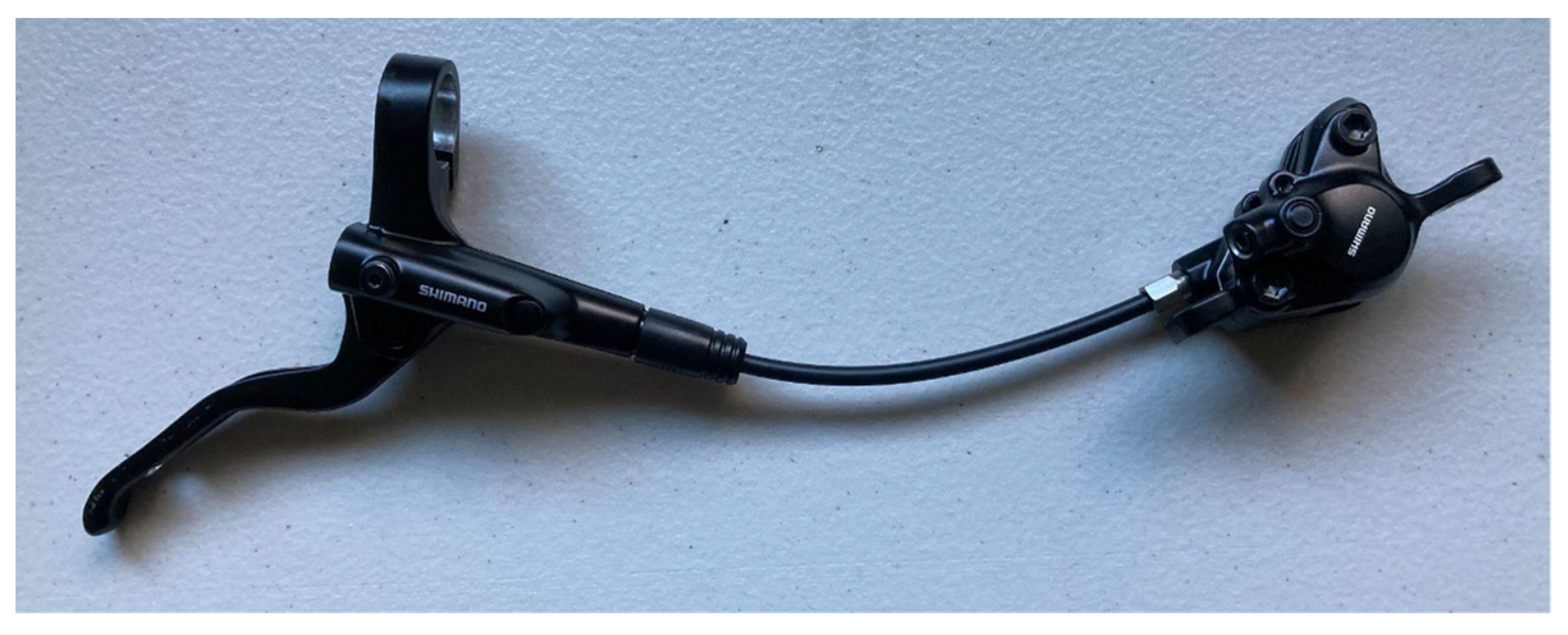
An initial experiment was conducted with low-cost hardware to see what loads would be experienced if using only a single brake lever per caliper. Through this, it was determined that a 2500 N maximum compression load cell would be sufficient for the caliper force measurement. Next, a pressure gauge was installed in the system to characterize the lever force-to-pressure ratio. From this, it was determined that the hydraulic line pressure would not exceed 10 MPa at maximum lever force. The S-beam tension load cell was selected based on the ISO and CPSC standard maximum lever force of 180 N and 178 N, respectively. The selected sensor details can be found in Table A1.
Table A1. Sensor name, model, maximum operating range, and absolute accuracy.
SensorModelRangeAccuracy
S-beam tension load cellDYLY-1030–300 N±1.5%
Button compression load cellFX290–2500 N3.5%
Pressure transducerMSP3000–17.2 MPa±1.0%
The test data was collected with an Arduino UNO R3 running through the Arduino IDE software. All four sensors output a 0 to 20 mV/V analog signal. This signal was amplified to 0 to 5 V for the Arduino through an HX711 Wheatstone Bridge Amplifier. Due to the force on each button load cell being close to the max range, the amplification signal saturated the input of the Arduino data acquisition unit. A voltage divider was used to decrease the output signal down to the 0 to 5 V range. The circuit wiring diagram is presented in Figure A2.
Figure A2. Circuit diagram used for the test setup.
Applsci 13 01767 g0a2
The pressure transducer was calibrated with an analog pressure gauge in the same system. The tension load cell was calibrated by hanging masses of known weight, and the compression load cells were calibrated by added known mass to a custom calibration fixture.

Appendix B. Testing Results from Prototype Iterations

Caliper force and lever pressure as a function of lever force for the prototype system with the valve in the open and closed position are shown in Figure A3. The advertised maximum brake pressure reduction from open to closed for this valve was 57%, and our measurements showed a reduction of 56%. This proportioning valve provides equal front and rear braking at low pressures, then decreases the caliper force at high pressures.
Figure A3. Caliper compression force and system pressure as a function of lever force for the prototype with the proportioning valve open (left) and closed (right).
Applsci 13 01767 g0a3
The experimental results show a different pressure profile during lever application than lever release indicating a source of system hysteresis (Figure A4). The arrows show the direction of the hysteresis loop for both lever application and lever release. Rotor-to-pad spacing, pressure transducer expansion, trapped air, hose expansion, viscous drag, piston retraction, and sensor restoration delay were all investigated as potential reasons for the hysteresis displayed in the results.
Figure A4. Caliper force and line pressure as a function of lever force. The arrows show the direction of the hysteresis loop.
Applsci 13 01767 g0a4
The first hysteresis variable to be eliminated was rotor-to-pad spacing. This is defined as the air gap between the brake pads and the brake rotor. If there is a mismatch between the gap in the front brake setup and the rear brake setup, then one brake caliper will engage the brake rotor before the other. Not only will this cause a situation where there is a differential pressure between the calipers during lever application and lever release, but this could also change the level of proportioning depending on the air gap. Multiple tests were run with varying rotor-to-pad measurements by inserting shims between the caliper and the pad. For all iterations of the rotor-to-pad spacing, the hysteresis did not change.
Another potential cause of hysteresis in the results was an expansion from the pressure transducer. If the pressure transducer changes volume as a function of pressure, anytime pressure is decreased, the volume may not be restored in the same amount of time due to material properties, thus causing the hysteresis loop. This was tested by removing the pressure transducer and then running the same test again; however, the results did not change.
This hysteresis can also occur when there is air trapped in the system. The air pockets are compressed before the system pressure increases and then expand when the system pressure is released. A time delay between lever release and pressure decrease occurs when these air pockets expand, potentially causing the hysteresis loop. This was eliminated as a potential source of hysteresis by using the shortened test setup shown in Figure A5. This shortened brake system decreases the chances of having air trapped in the system; however, there was no change in the results.
Figure A5. Shortened brake system to eliminate potential hysteresis due to trapped air and hose expansion.
Applsci 13 01767 g0a5
A shortened brake system also decreases the potential hysteresis due to hose expansion. At high lever force, the hose can expand, which increases the system volume and decreases the output force. As the lever is released, the line pressure stays elevated as the hose contracts, and the system volume decreases, but, as before, there was no change in the results.
Another culprit may be viscous drag creating a time delay in pressure response. As the fluid flows through the hose, it takes time to flow, so the decrease in pressure is not instantaneous. To test this, different lever application speeds were investigated, with no change in the results. Another form of drag in the system comes from the piston seals. As the pistons retract, the drag from the seals can cause a time delay in the pressure decrease, potentially causing the hysteresis seen. This was tested by shimming the system so that there was no piston displacement; however, there was still no change in the results.
The details of the final iteration of the prototype are available in Section 4.2.

References

  1. Hadland, T.; Lessing, H.-E.; Clayton, N.; Sanderson, G.W. Bicycle Design: An Illustrated History; MIT Press: Cambridge, MA, USA, 2014. [Google Scholar]
  2. Borgeson, G. Duesenberg-The J Is Born. In Errett Lobban: His Empire, His Motor Cars; Automobile Heritage Publishing & Co: New Albany, IN, USA, 2005; p. 40. [Google Scholar]
  3. Wilson, D.G.; Schmidt, T. Bicycling Science; MIT Press: Cambridge, MA, USA, 2020. [Google Scholar]
  4. Centers for Disease Control and Prevention. WISQARS, 2020. Available online: https://wisqars.cdc.gov/nonfatal-reports (accessed on 12 February 2022).
  5. Global E-Bike Sales by Year-Institute for Transportation and Development Policy. Available online: https://www.itdp.org/2020/02/04/will-e-bikes-make-cycle-highways-happen/global-e-bike-sales-by-year/ (accessed on 3 December 2021).
  6. Toll, M. The US Is Doubling E-Bike Imports This Year to Half a Million, and Even That Isn’t Enough. 2020. Available online: https://electrek.co/2020/10/28/the-us-is-doubling-e-bike-imports-this-year-to-half-a-million-and-even-that-isnt-enough/ (accessed on 3 December 2021).
  7. Huertas-Leyva, P.; Dozza, M.; Baldanzini, N. E-bikers’ braking behavior: Results from a naturalistic cycling study. Traffic Inj. Prev. 2019, 20, 62–67. [Google Scholar] [CrossRef] [PubMed]
  8. Lie, D.; Sung, C.-K. Synchronous brake analysis for a bicycle. Mech. Mach. Theory 2010, 45, 543–554. [Google Scholar] [CrossRef]
  9. Klug, S.; Moia, A.; Verhagen, A.; Görges, D.; Savaresi, S.M. Effectiveness of Actuating on Rectilinear Bicycle Braking Dynamics. IFAC-Pap. 2017, 50, 972–979. [Google Scholar] [CrossRef]
  10. Maier, O.; Györfi, B.; Wrede, J.; Arnold, T.; Moia, A. In-depth analysis of bicycle hydraulic disc brakes. Mech. Syst. Signal Process. 2017, 95, 310–323. [Google Scholar] [CrossRef]
  11. Maier, O.; Pfeiffer, M.; Wrede, J. Development of a Braking Dynamics Assistance System for Electric Bicycles: Design, Implementation, and Evaluation of Road Tests. IEEE/ASME Trans. Mechatron. 2015, 21, 1671–1679. [Google Scholar] [CrossRef]
  12. Corno, M.; D’Avico, L.; Panzani, G.; Savaresi, S.M. A haptic-based, safety-oriented, braking assistance system for road bicycles. In Proceedings of the 2017 IEEE Intelligent Vehicles Symposium (IV), Los Angeles, CA, USA, 11–14 June 2017; pp. 1189–1194. [Google Scholar] [CrossRef]
  13. Corno, M.; Panzani, G.; Savaresi, S.M.; Todeschini, F. Brake Assist System for a Cyclist on a Bicycle by a Haptic Feedback. U.S. Patent 10,293,878 B2, 21 May 2019. [Google Scholar]
  14. Mao, Y.J.; Tseng, C.H. A Study of a Pressure Regulator for an Anti-Lock Braking System for Low-Powered Vehicles. Proc. Inst. Mech. Eng. 2004, 218, 793. [Google Scholar] [CrossRef]
  15. Corno, M.; D’Avico, L.; Savaresi, S.M. An Anti-Lock Braking System for Bicycles. In Proceedings of the 2018 IEEE Conference on Control Technology and Applications (CCTA), Copenhagen, Denmark, 21–24 August 2018; pp. 834–839. [Google Scholar] [CrossRef]
  16. Klug, S.; Moia, A.; Verhagen, A.; Görges, D.; Savaresi, S. The influence of bicycle fork bending on brake control. Veh. Syst. Dyn. 2021, 59, 375–395. [Google Scholar] [CrossRef]
  17. Hua, C.-C.; Kao, S.-J. Design and implementation of a regenerative braking system for electric bicycles based on DSP. In Proceedings of the 2011 6th IEEE Conference on Industrial Electronics and Applications, Beijing, China, 21–23 June 2011; pp. 703–707. [Google Scholar] [CrossRef]
  18. Lin, C.-L.; Hsieh, M.-C.; Chen, T.-H. Integrated Driving and Braking Control Unit for Electric Bikes. SAE Int. J. Veh. Dyn. Stab. NVH 2018, 2, 223–242. [Google Scholar] [CrossRef]
  19. Debraux, P.; Grappe, F.; Manolova, A.V.; Bertucci, W. Aerodynamic drag in cycling: Methods of assessment. Sport. Biomech. 2011, 10, 197–218. [Google Scholar] [CrossRef] [PubMed]
  20. CPSC. Requirements for Braking System, 16 CFR 1512.5. 2019. Available online: https://www.ecfr.gov/current/title-16/chapter-II/subchapter-C/part-1512/subpart-A/section-1512.5 (accessed on 26 November 2021).
  21. ISO. Cycles-Safety Requirements for Bicycles, Part 2: Requirements for City and Trekking, Young Adult, Mountain and Racing Bicycles; BSI Standards Publication: London, UK, 2015. [Google Scholar]
  22. Lieh, J. Closed-Form Method to Evaluate Bike Braking Performance. Available online: https://www.google.com.hk/url?sa=t&rct=j&q=&esrc=s&source=web&cd=&ved=2ahUKEwj97NvY1e78AhUX7zgGHdMIDZ0QFnoECAwQAQ&url=https%3A%2F%2Fhupi.org%2FHPeJ%2F0019%2FClosed-form-braking-bike-2.pdf&usg=AOvVaw1GnUqwStS6HtAxpWto-NpV (accessed on 26 November 2021).
  23. Maier, O.; Pfeiffer, M.; Scharpf, S.; Wrede, J. Conditions for nose-over and front wheel lockup of electric bicycles. In Proceedings of the 17th International Conference on Research and Education in Mechatronics (REM), Compiegne, France, 15–17 June 2016; pp. 219–224. [Google Scholar] [CrossRef]
  24. Famiglietti, N.; Nguyen, B.; Fatzinger, E.; Landerville, J. Bicycle Braking Performance Testing and Analysis. In SAE Technical Paper Series; SAE International: Warrendale, PA, USA, 2020. [Google Scholar] [CrossRef]
  25. MathWorks Documentation. Longitudinal Wheel; The MathWorks, Inc.: Nantick, MA, USA, 2022. [Google Scholar]
  26. Pacejka, H. Tire and Vehicle Dynamics; Butterworth-Heinemann: Portsmouth, NH, USA, 2012. [Google Scholar]
  27. Maier, O.; Hillenbrand, S.; Wrede, J.; Freund, A.; Gauterin, F. Vertical and Longitudinal Characteristics of a Bicycle Tire. Tire Sci. Technol. 2018, 46, 153–173. [Google Scholar] [CrossRef]
  28. Dunlap, C., III; Jordan, B. Braking System for a Bicycle. U.S. Patent 10,913,510, 9 February 2021. [Google Scholar]
  29. purdueMET. Measuring Mass Moment of Inertia of a Wheel-Brain Waves. 2016. Available online: https://www.youtube.com/watch?v=MnrCfa4DOvc (accessed on 26 November 2021).
  30. Meijaard, J.; Papadopoulos, J.M.; Ruina, A.; Schwab, A. Linearized dynamics equations for the balance and steer of a bicycle: A benchmark and review. Proc. R. Soc. A Math. Phys. Eng. Sci. 2007, 463, 1955–1982. [Google Scholar] [CrossRef]
  31. Cossalter, V. Motorcycle Dynamics, 2nd ed.; Lulu Press: Durham, NC, USA, 17 September 2006. [Google Scholar]
  32. Shimano, K.; Fujii, Y. Hydraulic Bicycle Brake System. U.S. Patent 3,554,334, 12 January 1971. [Google Scholar]
  33. Zinn, L. Technical FAQ: Derailleurs, Brakes, and Frame Fatigue. 2018. Available online: https://www.velonews.com/gear/technical-faq-derailleurs-brakes-and-frame-fatigue/ (accessed on 1 May 2022).
  34. MacDermid, J.C.; Lee, A.; Richards, R.S.; Roth, J.H. Individual Finger Strength: Are the Ulnar Digits ‘Powerful’? J. Hand Ther. 2004, 17, 364–367. [Google Scholar] [CrossRef] [PubMed]
  35. Jan Heine, N.H. (Ed.) Bicycle Quarterly; Bicycle Quarterly Press: Seattle, WA, USA, 2008. [Google Scholar]
Figure 1. Test layout for the prototype hydraulic brake system with proportioning. This includes force and pressure sensors along with the data acquisition equipment.
Applsci 13 01767 g001
Figure 2. Brake pressure over time for a rider performing an emergency stop. Data points labeled “Simulation” show the hyperbolic tangent curve fit.
Applsci 13 01767 g002
Figure 3. Locations of the dimensions described in Table 2 relative to the center of mass and ground plane.
Applsci 13 01767 g003
Figure 4. Stopping distance velocity profiles for front, rear, and both brake applications comparing analytical results to simulated results.
Applsci 13 01767 g004
Figure 5. Comparison of wheel speed during a braking event for the simulation and for sensor data provided by Klug et al. [9]. Braking pressure was equal front and rear. The discrepancy at 0.5 s may indicate an incorrect simulation model or research data.
Applsci 13 01767 g005
Figure 6. Maximum front and rear braking force profiles for the varying center of mass position (acm/hcm) [8]. The blue line with asterisks shows the braking profile of the equal front and rear brake pressure. Dotted lines delineate the deceleration rate.
Applsci 13 01767 g006
Figure 7. Bench-top prototype brake system including a proportioning valve and pressure transducer (force sensors omitted). Mass, as shown, is 0.85 kg.
Applsci 13 01767 g007
Figure 8. Caliper force as a function of lever force before (left) and after (right) correcting for caliper load cell sensor hysteresis.
Applsci 13 01767 g008
Figure 9. Raw test result data of front and rear brake force for lever application only with varying levels of proportioning.
Applsci 13 01767 g009
Figure 10. Graph showing the mathematical model of the proportioning valve used in the simulation model.
Applsci 13 01767 g010
Figure 11. Critical tire coefficient of friction at tip-over for the varying center of mass positions and road gradients defining the region at which tip-over may occur. Tire coefficient of friction is shown by the colored lines, with values increasing with the color gradient from red to blue.
Applsci 13 01767 g011
Figure 12. Minimum tire coefficient of friction before front wheel lock occurs for the bike and rider center of mass position ratio and road downslope gradient. Tire coefficient of friction is shown by the colored lines, with values increasing with the color gradient from red to blue.
Applsci 13 01767 g012
Figure 13. Simulated stopping distance without wheel-lock (m) from 25 km/h for a 100 kg bike and rider system comparing the single-lever, prototype proportioning brake system versus a dual-lever brake system.
Applsci 13 01767 g013
Figure 14. Percent decrease in stopping distance for the prototype brake system showing an increased advantage for high centers of mass and when riding on steeper downslopes.
Applsci 13 01767 g014
Figure 15. Stopping distances for the prototype proportioning system and an ideal proportioning system with rear tire normal force sensing. For values of acm/hcm below 0.9, the stopping distance becomes limited by tip-over.
Applsci 13 01767 g015
Figure 16. Percent decrease in stopping distances for an ideal proportioning valve with rear-wheel normal force sensing versus the prototype system showing the greatest advantage shown on steep downslopes and lower C.O.M. ratios.
Applsci 13 01767 g016
Figure 17. Failure mode of the proportioning valve lower seal during reliability testing.
Applsci 13 01767 g017
Table 1. Comparison of ISO and CPSC tests. Values for the ISO column are requirements for city bicycles in dry conditions. The CPSC braking distance has been corrected to match the ISO 25 km/h velocity and 100 kg mass [20,21].
SpecificationsISOCPSC
Braking distance7.00 m5.61 m
Maximum lever force180 N178 N
Brake lever maximum distance from handlebar90 mm89 mm
Distance of applied test force from end of brake lever25 mm25 mm
Test track maximum gradient±0.5%±1.0%
Test track coefficient of friction with tire>0.75<1.0
Wind speed during testing<3 m/s<3.1 m/s
Number of test runs54
Table 2. Values selected for each variable used in the bicycle longitudinal dynamics and bicycle tire simulation blocks during corroboration tests.
VariableValueUnitsNotes
m100 *kgBike and rider combined mass
acm0.7 *mDistance from center of mass to front tire contact patch
bcm0.4 *mDistance from center of mass to rear tire contact patch
hcm1.1 *mHeight of center of mass from ground plane
Cd0.3 Coefficient of drag for bike with rider
Af1.1 *m2Frontal area of bike with rider
Iyy0.16kg·m2Mass-moment of inertia of each wheel
Lrel0.6mTire relaxation length (tire response time)
Re0.35mLoaded tire radius
μkinetic0.5 Brake pad and rotor coefficient of friction
dbore0.03mBrake caliper piston bore diameter
Rm0.085mMean rotor radius
V024 *km/hVelocity at initiation of braking
* These values were altered for each corroboration test.
Table 3. Maximum deceleration ( x ¨ ) at the point of tip-over for the varying center of mass from the front axle (acm) and center of mass height from the ground plane (hcm) [23].
Rider Typeacm (m)hcm (m) x ¨ critical   ( g ) x ¨ simulation   ( g ) Difference
Male5th percentile0.6110.8660.7060.7080.35%
50th percentile0.6400.9200.6960.6980.34%
90th percentile0.6830.9980.6840.6870.38%
Female5th percentile0.6040.8010.7540.7550.12%
50th percentile0.6220.8420.7390.7400.17%
90th percentile0.6400.9130.7010.7030.29%
Table 4. Measured and referenced model parameters used for simulating the braking performance of an e-bike.
VariableValueUnitsNotes
m104kgBike and rider combined mass with a 68 kg rider
acm0.70mDistance from center of mass to front tire ground contact
bcm0.41mDistance from center of mass to rear tire ground contact
hcm0.54mHeight of center of mass from ground plane
Cd *1.15 Coefficient of drag for bike with rider
Af *0.61m2Frontal area of bike with rider
Iyyf0.12kg·m2Mass-moment of inertia, front wheel
Iyyr0.15kg·m2Mass-moment of inertia, rear wheel
Lrel *0.6mTire relaxation length (tire response time)
Re0.32mLoaded tire radius
μkinetic *0.5 Brake pad and rotor coefficient of friction
dbore0.021mBrake caliper piston bore diameter
Rm0.072mMean rotor radius
* Referenced from literature.
Table 5. Combined CPSC and ISO stopping distance simulation test for the e-bike tested with and without the prototype proportioning system.
ConditionPrototype ProportioningNo ProportioningDifference
Dry5.17 m6.01 m15.0%
Wet5.39 m6.37 m16.7%
Table 6. Comparison of the CPSC and ISO test specifications against a simulation of the prototype system using the physical parameters of the e-bike detailed in Table 4.
SpecificationsISOCPSCPrototype
Braking distance7.00 m5.61 m5.17 m
Maximum lever force180 N178 N129 N
Brake lever maximum distance from handlebar90 mm89 mm80 mm
Distance of applied test force from end of brake lever25 mm25 mm25 mm
Test track maximum gradient±0.5%±1.0%0%
Test track coefficient of friction with tire>0.75<1.00.85
Wind speed during testing<3.0 m/s<3.1 m/s0 m/s
Disclaimer/Publisher’s Note: The statements, opinions and data contained in all publications are solely those of the individual author(s) and contributor(s) and not of MDPI and/or the editor(s). MDPI and/or the editor(s) disclaim responsibility for any injury to people or property resulting from any ideas, methods, instructions or products referred to in the content.

