Series PIDA Controller Design for IPDT Processes

Abstract

This paper discusses optimal design of the series proportional–integral–derivative–accelerative (PIDA) controller for integral-plus-dead-time (IPDT) plants. The article starts with the design of disturbance reconstruction and compensation based on proportional-derivative-accelerative (PDA) stabilizing controllers. It shows that by introducing positive feedback by a low-pass filter from the (limited) output of the stabilizing PDA controller, one gets disturbance observer (DOB) for the reconstruction and compensation of input disturbances. Thereby, the DOB functionality is based on evaluating steady-state controller output. This DOB interpretation is in full agreement with the results of the analysis of the optimal setting of the stabilizing PDA controller and of its expanded PIDA version with positive feedback from the controller output. By using the multiple real dominant pole (MRDP) method, it confirms that the low-pass filter time constant in positive feedback must be much longer than the dominant time constant of the stabilized loop. This paper also shows that the constrained PIDA controller with the MRDP setting leads to transient responses with input and output overshoots. Experimentally, such a constrained series PIDA controller can be shown as equivalent to a constrained MRDP tuned parallel PIDA controller in anti-windup connection using conditional integration. Next, the article explores the possibility of removing overshoots of the output and input of the process achieved for MRDP tuning by interchanging the parameters of the controller transfer function, which was proven as very effective in the case of the series PID controller. It shows that such a modification of the controller can only be implemented approximately, when the factorization of the controller numerator, which gives complex conjugate zeros, will be replaced by a double real zero. Neglecting the imaginary part and specifying the feedback time constant with a smaller approximative time constant results in the removal of overshoots, but the resulting dynamics will not be faster than for the previously mentioned solutions. A significant improvement in the closed-loop performance can finally be achieved by the optimal setting of the constrained series PIDA controller calculated using the performance portrait method. This article also points out the terminologically incorrect designation of the proposed structure as series PIDA controller, because it does not contain any explicit integral action. Instead, it proposes a more thorough revision of the interpretation of controllers based on automatic reset from the controller output, which do not contain any integrator, but at the same time represent the core of the most used industrial automation. In the end, constrained structures using automatic reset of the stabilizing controller output can ensure a higher performance of transient responses than the usually preferred solutions based on parallel controllers with integral action that, in order to respect the control signal limitation, must be supplemented with anti-windup circuitry. The excellent properties of the constrained series PIDA controller are demonstrated by an example of controlling a thermal process and proven by the circle criterion of absolute stability.

1. Introduction

A whole chain of discoveries, their further modifications, improvements and patents gradually led to the development of pneumatic controllers at the beginning of the twentieth century. Due to the internal structure of the controllers, they were the heart of industrial automation [1,2,3]. The most important part of the structure was a positive feedback from the overall output of the controller to the output of the proportional controller, which generated a signal (automatic reset) that served to eliminate the permanent control error caused by acting disturbances. Even before the beginning of World War II, there was a generalization of the mentioned control structure with a stabilizing proportional (P) and a proportional–derivative (PD) term, also called Pre-Act (Taylor Instrument Companies), or Hyper-Reset (Foxboro). The control structures with automatic reset were later interpreted as integrating controllers [4], since automatic reset acts like an integrator in the linear domain. The name change was originally attributed to disturbance compensation control of the temperature measured by the thermocouple. By getting the potentiometer of the measuring bridge with the null balancing method, the integration of the control error was achieved by summing the increments of the angle of the motor rotating with the potentiometer [1,2,3]. Although both control methods with explicitly integrating controller and with automatic reset can be equivalent under certain (linear) circumstances, the equivalence is lost when working with a saturating controller (actuator). Such problems in connection with equivalent controllers with integral action became clearly apparent during the transition to digitally implemented controllers by the occurrence of so-called undesired integration, also called integrator windup [5,6,7,8,9,10,11,12]. Although a number of different anti-windup controllers have been developed to address the problem, the evaluation of constrained structures based on the use of an automatic reset with a special parameterization of numerator terms of the PID controller in Ref. [13] proved to be more practical than the anti-windup structures based on integrating controllers [14]. Subsequently, the question was raised whether these useful properties could not be further improved by combining the automatic reset with a higher derivative-order controller, referred to as proportional–derivative–accelerative (PDA).

However, before we start to look at the structure of the PDA-based controller, we need to clarify the terminology. The original automatic reset controller is usually referred to as a series proportional–integral (PI) controller. Similarly, an automatic reset combined with a stabilizing PD controller (originally Pre-Act) is today called a series PID controller. If an automatic reset is added to the PDA controller, it could also be called a series PIDA controller. However, all of these designations are inherently illogical because the structure under consideration does not contain an explicit integrator. The confusing terminology is due to the fact that, for a whole century since the invention of the automatic reset, it was not noticed that it can also be interpreted as a disturbance observer for the reconstruction of input disturbances. The properties of the disturbance observer become clear when analyzing the steady states of controllers designed with integrating process models [15,16,17,18]. In this context, the terminology is also important from the point of view of controller tuning.

Many works deal with the optimal design of PIDA controllers, also known as PIDD2, PIDD${}^2$ or PIDC controllers [19,20,21,22,23,24,25,26,27,28,29,30,31,32,33]. The growing use of these controllers is the result of ever-growing demands on the performance of transients typically occurring especially in connection with speed control in high-end robotic and mechatronic applications.

One of the first attempts to obtain an analytical PIDA controller design procedure for a third-order system [19,20] neglected the effects of derivative filters required in the implementation of the controller transfer function. To determine the four parameters of the ideal series controller, four equations were solved using the root locus method. The proposed solution was based on the choice of a pair of complex conjugate poles of the closed loop, a real pole with the same real part and a real pole shifted to higher frequencies (resulting in negligible dynamics). The approach has been verified with different types of third-order plants and using different performance metrics such as percent overshoot, settling time and peak time. The setpoint responses of this approach typically exhibited overshoot, even without considering control signal limitations. In ref. [21], this approach was further modified by Kitti’s method to reduce overshoot and provide robust stability.

In ref. [23], the PIDD${}^2$ (i.e., PIDA) controller is presented as an alternative to fractional-order (FO) PID controllers (which are implemented by higher-order filters). The optimal setting of the four controller parameters for the automatic voltage regulator (AVR) of a synchronous generator was realized by minimizing the integral of the time-weighted absolute error (ITAE) using particle swarm optimization. Among the main implementation problems was the use of filters required to obtain the derivative and the second derivative of the control error signal. The use of PIDA control was extended with the aim of balancing the differences between the generated power and the constantly changing load demand in a power system from the AVR to the load frequency control (LFC). To achieve robust and reliable performance, the work proposed to optimize the parameters of the ideal parallel PIDA controller with soft computing techniques using ITAE criteria without considering the necessary filters and control signal constraints. The work [30] continues with the application of artificial intelligence methods. An optimal design of a PIDA controller for a higher-order nonlinear time-delay system using a modified butterfly optimization algorithm is proposed to achieve an optimal control response complemented by a mutuality system. The goal is to reduce overshoot due to large disturbances but the focus is on the computational aspects of the optimization. Filter and signals have not been investigated.

Another application of PIDA control with derivative filter was developed by [31] to improve the flight stability of a quad copter in a noisy environment. It is associated with a heuristic genetic filter design that addresses the challenges of nonlinearity, uncertainties, coupling and measurement noise that cause instability in flight and in automatic hover. The tuning of the proposed parallel PIDA controller with multiple inputs and outputs is performed by a stochastic dual simplex algorithm.

Despite the fact that the controller’s filter has a significant impact on the closed-loop stability [34], the filters required for a reliable implementation of PIDA controllers in practice have not yet been studied in detail. For this reason, ref. [28] considered designing a PIDA controller using an interactive tool for designing a parallel PIDA controller with minimum order filters in the derivative and acceleration terms. However, such an approach unnecessarily increased the number of controller parameters and did not allow the design of a controller for signal limitations. Furthermore, similarly to in Ref. [35], with two additional filter parameters, the complexity of controller tuning increases.

The authors of [25] recognized the importance of controller filters in terms of circuit robustness and considered the time constant of the first-order filter as a tuning parameter in their design of an IMC-PIDA controller for an interconnected time-delayed power system. In Ref. [26], an optimal low-pass filter is combined with each derivative term of an IMC-PIDA (PIDD2) controller applied to a dual rotor aerodynamic system. The parameters of the PIDA controller for controlling the output voltage of a non-ideal dc–dc converter were obtained using a modified Gray-Wolf optimizer [27].

In ref. [32] the authors deal with the detailed modeling and design of load frequency controllers (LFCs) of single and multi-area power systems using PID controllers and PID controllers with serial compensators. These controllers, referred to as PIDC, can be considered equivalent to PID controllers with higher-order derivatives (PIDA controllers are equivalent to PIDC1 control). The explicit tuning formulas for the different turbine types are characterized by the use of two free parameters that affect the performance and robustness of the system. They define a single and a triple real pole of a closed-loop control system and the corresponding poles and zeros of the controller under study. The integral performance measures IAE and ITAE, the total variation TV used to evaluate the control effort, and the sensitivity indices derived by simulations and calculations (maximum sensitivity $M_s$, maximum complementary sensitivity $M_p$ and measurement noise sensitivity $M_n$) are analyzed in terms of these tuning parameters. The parallel PIDD2 controller combined with a second-order binomial filter [33] for the automatic voltage regulator (AVR) of a synchronous generator is designed by minimizing the load disturbance response while considering the constraints on the sensitivity functions: $M_s$, $M_p$ and $M_n$. The five controller parameters are obtained by iteratively solving the optimization problem for given sensitivities $M_s$ and $M_n$ and for a fixed value of controller zeros damping factor $\xi$. The robustness index $M_p$ is then calculated using the auxiliary parameter $\xi$. Although several limitations of the internal signals are mentioned in the description of the AVR control process, the experiments performed were linear.

Several approaches are based on setting the multiple real dominant poles [14,36]. Other solutions [37,38] propose conditions for the maximum decay rate. The paper shows that the formulation of conditions for the closed-loop poles can be avoided by considering the performance portrait method. The method can be advantageous both with regard to the transcendental nature of a closed circuit with an infinite number of poles and also with regard to the nonlinear character due the control signal limitations.

In this context, the paper is organized as follows. Section 2 summarizes the main results of the design of an ideal PDA controller for the IPDT system using the multiple real dominant poles method, its extension by a prefilter and low-pass implementation filters. Section 3 extends the problem to the series PIDA controller with a simple disturbance-observer-based disturbance reconstruction and a compensation of the disturbance by a positive feedback from the controller output. This section also includes a brief analysis of the problems caused by saturation of the control signal. In Section 4, the optimal tuning of the PIDA controller is performed using the performance portrait method and illustrated by an example of controlling a thermal process. Absolute stability of the loops with modified PIDA controllers are proven by the circle criterion in Section 5. The main results of the work are discussed in Section 6, emphasizing the superior properties obtained by reliable controller tuning and in the saturating control. A paper summary and future developments are included in the conclusions.

2. Tuning of PDA Controllers for IPDT Plant

In this paper, the velocity of the transients is evaluated using the absolute integral error

$$IAE={\int }_0^{\infty }\left|e\left(t\right)\right|dt;e=w-y$$

(1)

To keep the paper short, the evaluation deals only with the step responses of the input disturbance, with all corresponding performance values denoted by the subscript “d”.

For the process output $y\left(t\right)$ and the controller output $u\left(t\right)$, the robustness analysis will focus on an IPDT process model described by the transfer function

$$S\left(s\right)=\frac{Y\left(s\right)}{U\left(s\right)}=S_0\left(s\right)e^{-T_{dp}s};S_0\left(s\right)=\frac{K_{sp}}{s}$$

(2)

with a gain $K_{sp}$ and a dead time $T_{dp}$. In the “optimal” controller tuning, the omitted plant model index “p” corresponds to the “nominal” model parameters $K_s$ and $T_d$.

For the dead time present in the loop, the design of stabilizing controllers can be carried out by the multiple-real-dominant-pole (MRDP) method [39]. An ideal stabilizing proportional–derivative–accelerative (PDA) controller with the gains $K_p,K_d,K_a$ [40] is given by

$$R\left(s\right)=K_p+K_{d}s+K_a{s}^2$$

(3)

when

$$u\left(t\right)=K_p(w-y)-K_d\dot{y}-K_a\ddot{y}$$

(4)

yields for a nominal plant with parameters $K_s$ and $T_d$ the closed-loop transfer function

$$F_c\left(s\right)=\frac{R\left(s\right)S\left(s\right)}{1+R\left(s\right)S\left(s\right)}=\frac{K_s(K_p+K_{d}s+K_a{s}^2)}{s{e}^{T_{d}s}+K_s{K}_a{s}^2+K_s{K}_{d}s+K_s{K}_p}$$

(5)

2.1. Quadruple Real Dominant Pole Controller Tuning

From the characteristic quasi-polynomial

$$A\left(s\right)=s{e}^{T_{d}s}+K_s{K}_a{s}^2+K_s{K}_{d}s+K_s{K}_p$$

(6)

the condition of quadruple real dominant pole $s_o$ can be formulated as follows

$${\left\{A\left(s\right);\frac{d}{ds}A\left(s\right);\frac{d^2}{d{s}^2}A\left(s\right);\frac{d^3}{d{s}^3}A\left(s\right)\right\}}_{s=s_o}=\mathbf{0}$$

(7)

From

$$\frac{d^3}{d{s}^3}A\left(s\right)=[s{T}_d^3+3T_d^2]e^{T_{d}s}=0$$

(8)

one gets optimal values of the dominant pole and the dominant closed-loop time constants as

$$s_o=-3/T_d;T_o=-1/s_o=T_d/3$$

(9)

From the remaining conditions (7) then follow the “optimal” controller parameters

$$K_{po}={\displaystyle \frac{27}{2K_s{T}_d{e}^3}}={\displaystyle \frac{0.6721}{K_s{T}_d}};K_{do}={\displaystyle \frac{5}{K_s{e}^3}}={\displaystyle \frac{0.2489}{K_s}};K_{ao}={\displaystyle \frac{T_d}{2K_s{e}^3}}={\displaystyle \frac{0.0249T_d}{K_s}}$$

(10)

If we introduce the controller time constants using

$$T_D=K_d/K_p=0.3704T_d;T_A^2=K_a/K_p=0.0370T_d^2$$

(11)

we can further introduce a pre-filter $F_p\left(s\right)$, the task of which is to cancel the zeros from the $F_c\left(s\right)$ (5)

$$F_p\left(s\right)=\frac{b_2{s}^2+b_{1}s+1}{T_A^2{s}^2+T_{D}s+1}$$

(12)

and possibly also some of the closed-loop poles $s_o$ (time constants $T_o$). In the simplest but the most robust case, one can choose

$$b_2=0;b_1=0;$$

(13)

Setpoint step responses can be accelerated by selecting the $F_p$ numerator so that it cancels one closed-loop pole $s_o=-1/T_o$

$$b_2=0;b_1=T_o;$$

(14)

Two closed-loop dominant time constants $T_o$ can be cancelled by the numerator tuning

$$b_2=T_o^2;b_2=2T_o;$$

(15)

2.2. Implementation and Noise Attenuation Low-Pass Filters

To get proper controllers and at the same time achieve appropriate damping of the measurement noise, the ideal PDA transfer function has to be combined with binomial low-pass filter $Q_n\left(s\right)$ with the relative degree $n\ge 2$

$$\begin{array}{c}{Q}_n\left(s\right)=Y_f\left(s\right)/Y_m\left(s\right)=1/{\left(T_{f}s+1\right)}^n=1/P_n\left(s\right)\end{array}$$

(16)

Fixed with already specified n and $T_f$, $Q_n\left(s\right)$ expressing the necessary filtration of the measured output $y_m\left(t\right)$ can be taken into account and included into the system’s step response [13]. Then, the index “f” of its output $y_f\left(t\right)$ can be omitted. This means that the output of the filter is considered directly as the output value of the controlled system.

If you need to search the filter parameters interactively and adapt the PIDA parameter proposal to the selected filter settings for a system, given by the IPDT model transfer function (2), the additional filter delay can be considered by a chosen delay equivalence [41], when the total loop dead time $T_d$ consists of an estimate of the process delay $T_{dp}$ (representing the sum of the process, actuator and measurement sensor delays with a communication and computation delay) and an intentionally introduced equivalent filter delay estimate $T_e$

$$T_d=T_{dp}+T_e$$

(17)

approximated as (see, e.g., [15,41])

$$T_e=nN{T}_f$$

(18)

The coefficient N can be specified by values ranging from $N=0.5$ (equivalence based on “half rule”) to $N=1$ (equivalence based on “average residence time”).

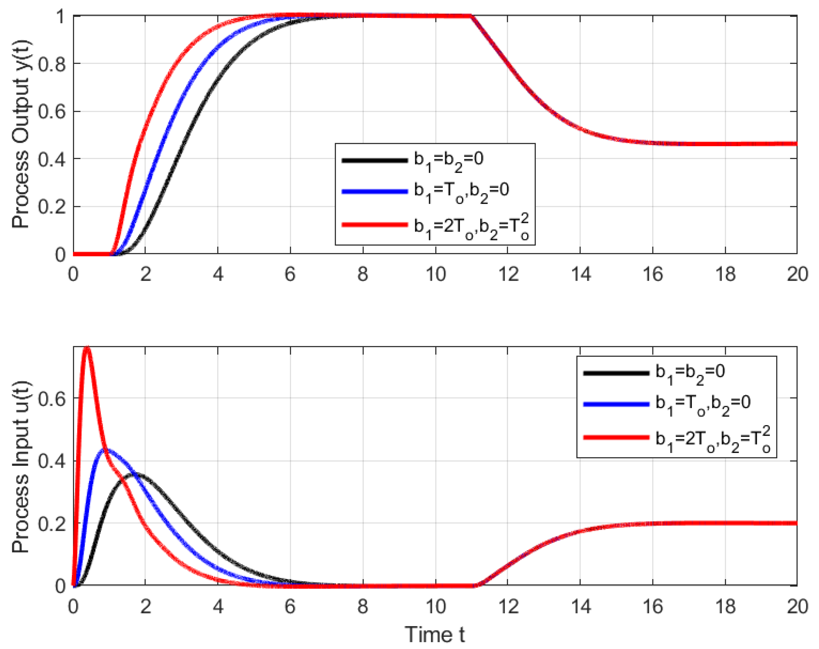
2.3. Illustrative Examples of PDA Control

Figure 1 shows an example of setpoint and disturbance step responses for an IPDT process ($T_{dp}=1$) and a PDA controller with different prefilter tuning completed by a fourth-order filter with $T_e=0.8$ tuned by the average residence time equivalence $T_e=4T_f$.

When wishing to compensate for piecewise constant input disturbances $d_i\in [-0.2,0]$, the control signal constraints must allow the compensating signal $-d_i$ to be set and at the same time leave a sufficient reserve for imposing the required dynamics of the circuit, i.e., to fulfill for all considered $d_i$ the conditions $U_{min}<-d_i<U_{max}$. Figure 2 shows an example of setpoint and disturbance step responses for an IPDT process ($T_{dp}=1$) and a PDA controller with different prefilter tuning completed by a fourth-order filter with $T_e=0.8$ tuned by the average residence time equivalence $T_e=4T_f$ with the control signal constraints chosen as

$$U_{min}=-0.02;U_{max}=0.22;$$

(19)

Remark 1 

(Steady-state controller output). Note that for a fixed input disturbance value $d_i=const$ the steady-state controller output is equal to $-d_i$ in both constrained and unconstrained case.

Remark 2 

(Effect of control signal constraints). Under the impact of admissible input disturbances, the conditions of control signal constraints do not cause any deformations of transient responses; their nature does not change compared to unconstrained control; only their course is slowed down.

3. Analytical Tuning of Series PIDA Controller

On the basis of Remark 1, it might seem that the reconstruction of the acting disturbances can be very easily realized by evaluating the controller output in steady states. Evaluating the achievement of steady states, however, is far from a trivial matter [17,42], which is especially true when accounting for measurement noise. It can be avoided by filtering the controller output using a low-pass filter with a time constant $T_i$ long enough to smooth out control activities arising during process stabilization. In the case of stable processes, it is then possible to assume that after a sufficiently long time the filter output is dominated by the steady-state value of the controller output.

By introducing a disturbance observer in the form of a low-pass filter $1/(1+T_{i}s)$ connected to the (possibly saturated) output of the controller and compensating the reconstructed disturbance at the output of the stabilizing PDA controller, the overall transfer function of the controller changes in the proportional zone of control to

$$R\left(s\right)=\frac{(K_p+K_{d}s+K_a{s}^2)(1+T_{i}s)}{T_{i}s}$$

(20)

Despite the terminology reservations, in the following we will call this structure the series PIDA controller (Figure 3). For a nominal plant with parameters $K_s$ and $T_d$ the closed-loop transfer function is

$$F_c\left(s\right)=\frac{R\left(s\right)S\left(s\right)}{1+R\left(s\right)S\left(s\right)}=\frac{(K_s{K}_a{s}^2+K_s{K}_{d}s+K_s{K}_p)(1+T_{i}s)}{s^2{T}_i{e}^{T_{d}s}+(K_s{K}_a{s}^2+K_s{K}_{d}s+K_s{K}_p)(1+T_{i}s)}$$

(21)

3.1. Quintuple Real Dominant Pole Controller Tuning

The characteristic quasi-polynomial now changes to

$$A\left(s\right)=s^2{T}_i{e}^{T_{d}s}+(K_s{K}_a{s}^2+K_s{K}_{d}s+K_s{K}_p)(1+T_{i}s)$$

(22)

and the increased number of controller parameters requires increasing the multiplicity of the dominant pole considered to 5. From the fourth derivative of $A\left(s\right)$ equivalent to (8) it is now possible to calculate two values $-6/T_d$ and $-2/T_d$. Of them, however, only the second one meets the conditions of a dominant pole $s_o$, thus

$$s_o=-2/T_d;T_o=-1/s_o=T_d/2$$

(23)

Evidently, the introduction of the disturbance observer slowed down the closed-loop transient responses. They are now characterized by the quadruple time constant $T_o=T_d/2$ instead of the triple time constant $T_o=T_d/3$ (9). The remaining controller parameter can now be calculated as

$$K_{po}={\displaystyle \frac{0.932273}{K_s{T}_d}};K_{do}={\displaystyle \frac{0.388543}{K_s}};K_{ao}={\displaystyle \frac{0.045112T_d}{K_s}};T_i=2.583231T_d$$

(24)

Remark 3 

(Comparison of PDA and series PIDA controller parameters). In addition to the fact that the absolute optimal values of the $K_p$, $K_d$ and $K_a$ coefficients of the PDA controller have increased, which is reflected in the higher amplification of the measurement noise, it should be noted that, with respect to $T_o=T_d/3$ (9), the value of $T_i\approx 2.6T_d>>T_o=T_d/3$ ($T_i$ is more than seven times larger). From the point of view of the dynamics of transient responses characterized by the value $T_o$ of PDA control, we can therefore speak with sufficient accuracy about the reconstruction of the disturbance from steady-state controller output.

3.2. Prefilter Design

If we again introduce the controller time constants

$$T_D=K_d/K_p=0.4168T_d;T_A^2=K_a/K_p=0.0484T_d^2$$

(25)

we can further introduce a pre-filter $F_p\left(s\right)$, the task of which is to cancel the zeros from the $F_c\left(s\right)$ (21)

$$F_p\left(s\right)=\frac{b_3{s}^3+b_2{s}^2+b_{1}s+1}{(T_A^2{s}^2+T_{D}s+1)(T_{i}s+1)}$$

(26)

and possibly also some of the closed-loop poles $s_o$ (time constants $T_o$). In the simplest and the most robust case, one can choose

$$b_3=0;b_2=0;b_1=0;$$

(27)

Setpoint step responses can be accelerated by selecting the $F_p$ numerator so that it cancels one closed-loop time constant $T_o=-1/s_o=T_d/2$ (23)

$$b_3=0;b_2=0;b_1=T_o;$$

(28)

Two closed-loop dominant time constants $T_o$ can be cancelled by the numerator tuning

$$b_3=0;b_2=T_o^2;b_2=2T_o;$$

(29)

Three closed-loop dominant time constants $T_o$ could be cancelled by the numerator tuning

$$b_3=T_o^3;b_2=3T_o^2;b_2=3T_o;$$

(30)

We will expect the highest parametric sensitivity from this solution, which will manifest itself at least at shorter values of the equivalent delay $T_e$ used when setting the low-pass filters $Q_n\left(s\right)$ (16).

3.3. Illustrative Examples of PIDA Control

Figure 4 shows example of setpoint and disturbance step responses for an IPDT process ($T_{dp}=1$) and a PIDA controller with different prefilter tuning completed by a fourth-order filter with $T_e=0.8$ tuned by the average residence time equivalence $T_e=4T_f$. Control signal (process input) $u\left(t\right)$ serves in the first phase of transients to stabilize the output around the new setpoint signal value $w=1$. Because this signal also enters the disturbance observer, a “phantom” disturbance signal is reconstructed at its output with a delay given by the time constant $T_i$, despite the fact that no external disturbance actually occurs. By using a pre-filter with canceling of several poles of the closed circuit, the setpoint responses are accelerated, but the sensitivity of the circuit is also increased, which is also manifested in the partial deformation of the control signal transients at the fastest setting. From the point of view of the output, however, the responses remain monotonic after the setpoint change. After the disturbance step, the output monotonically returns to the required setpoint value with gradual reconstruction and compensation of the external disturbance value. The correct values of the external constant disturbance are reconstructed only after reaching a sufficiently close neighborhood of steady states.

When wishing to compensate for piecewise constant input disturbances $d_i\in [-0.2,0]$, the control signal constraints must allow the compensating signal $-d_i$ to be set and at the same time leave a sufficient reserve for imposing the required dynamics of the circuit, i.e., to fulfill for all considered $d_i$ with a sufficient margin the conditions $U_{min}<-d_i<U_{max}$. Figure 5 shows an example of setpoint and disturbance step responses for an IPDT process ($T_{dp}=1$) and a PIDA controller with different prefilter tuning completed by a fourth-order filter with $T_e=0.8$ tuned by the average residence time equivalence $T_e=4T_f$ with the control signal constraints chosen as (19). In the case of setpoint step responses, the limitations of the process input are manifested only when using pre-filters with canceling of several poles of the closed loop. The consequence of the limitation here is an overshoot of the output over the required setpoint value. In the case of disturbance step responses, when a significant part of the permissible range of process input is used up to compensate for an external disturbance, a substantial extension of transient length occurs. From the point of view of the control action transition from a fully saturated level to a steady state, the critical parameter of the controller is the size of the time constant $T_i$ [5,7]. From the shape of the transient of $u\left(t\right)$ with undershoot, which manifests itself during the output $y\left(t\right)$ with overshoot, it can be concluded that the value $T_i=2.583T_d$ (24) is too large.

Remark 4 

(Opposing requirements for choosing $T_i$). If we want to preserve the good properties of the stabilizing PDA controller even after the introduction of positive feedback with the time constant $T_i$, the value of $T_i$ must be as large as possible and, in addition, the coefficients $K_p,K_d$ and $K_a$ must be increased (to achieve a quintuple real dominant pole). However, to achieve high-quality transients with a limited control signal, the value of $T_i$ should be as small as possible.

Calculated controller transfer function (24) and (25) with complex polynomial zeros $T_A^2{s}^2+T_{D}s+1=0.0484s^{2}T{d}^2+0.4168Tds+1$

$$s_{1,2}=(-4.305785124\pm 1.456492874j)/Td,$$

(31)

however, does not give a direct possibility to choose some smaller time constant from the calculated parameters for $T_i$, as was the case in the design of the PID controller in Refs. [13,43]. The replacement of the constants appearing in the role $T_i$ can only be realized by neglecting the imaginary part of the pole (31), when we use the approximation

$$T_A^2{s}^2+T_{D}s+1\approx 0.0538s^2{T}_d^2+0.4640T_{d}s+1={(0.2320T_{d}s+1)}^2$$

(32)

In such a case, we recalculate parameters of the controller transfer function (24) as follows:

$$\begin{array}{c}{T}_i=0.2320T_d;K_p={\displaystyle \frac{0.9322730.232}{2.583K_s{T}_d}}={\displaystyle \frac{0.0837}{K_s{T}_d}};\hfill \\ T_D=2.583Td+0.232Td=2.815T_d;K_d=K_p{T}_D=0.2356/K_s;\hfill \\ T_A^2=2.583Td0.232T_d=0.599T_d^2;K_a=T_A^2{K}_p=0.0502T_d/K_s\hfill \end{array}$$

(33)

Transient responses in Figure 6 indicate the removal of output overshoots and control signal undershoots, thereby achieving the same number of monotonic sections of changes at the input and output as with transient responses without control signal saturation. However, setpoint step responses are somewhat slower than with unmodified controller parameters.

4. Calculation of the Series PIDA Controller for the IPDT System Using the Performance Portrait Method (PPM)

Since the imaginary part of the poles of the polynomial $T_A^2{s}^2+T_{D}s+1$ should be neglected to get a polynomial with real time constants applicable as $T_i$, the analytical re-tuning of the PIDA controller according to [13,43] provides limited performance. Although we can calculate the optimal controller settings using analytical methods just approximately, they are still useful, by offering simplifications and time savings, when we search for optimal solutions using numerical methods.

The core of the performance portrait method (PPM) is to search all relevant solutions and find the best one based on performance measures. An important advantage of numerical optimization of controller parameters based on a set (database) of system responses [44,45,46] is that it can be easily reused in case of changed specifications for the target system performance. In the first phase of the method, the transient responses are determined by simulation or experimentation on a real process with different relevant sets of control parameters. Then, the closed-loop step responses are evaluated using performance measures that approximate actual real-world requirements. The obtained data are stored in a set (database) of relevant solutions, also referred to as a performance portrait (PP). After creating a sufficiently large database, it is then relatively easy to find a controller that comes as close as possible to the expected desired performance. Of course, such a controller should be included in the final database of solutions.

An important performance specification is that the closed-loop responses should be as fast as possible, i.e., that the minimum $IAE$ value (1) for the setpoint and disturbance responses or their weighted combination is guaranteed. Furthermore, the selected controller should guarantee smooth process responses with a minimum number of monotonic intervals at the process input and output.

The estimation of the optimal parameters of the series PIDA controller can start with the modified parameter set (33). To simplify the notation, we introduce here dimensionless parameters

$$\begin{array}{c}{\tau }_i=T_i/T_d=0.2320;\kappa =K_p{K}_s{T}_d=0.0837;\hfill \\ {\tau }_D=T_D/T_d=2.815;{\tau }_A=\sqrt{T_A^2/T_d^2}=0.7741\hfill \end{array}$$

(34)

The actual experiments resulted in slightly modified parameters to obtain better transients. Optimal settings are finally found from the performance portrait corresponding to the parameter ranges

$$\begin{array}{c}\kappa \in [0.155,0.2];\Delta \kappa =0.005;\hfill \\ {\tau }_D\in [2.6,3.05];\Delta {\tau }_D=0.005;\hfill \\ {\tau }_A\in [0.75,0.87];\Delta {\tau }_A=0.015;\hfill \\ {\tau }_i\in [0.33,0.45];\Delta {\tau }_i=0.015;\hfill \end{array}$$

(35)

The differences in ${\tau }_i$ and $\kappa$ values are mainly due to the simplification in computing the initial parameter estimates (34).

To simplify the calculations, only one performance portrait based on unit disturbance steps with control signal constraints $U_{min}=-1.1;U_{max}=0.1$ was created for process gain $K_s=1$ and delay $T_{dp}=1$. The controller was implemented using the second-order filter ($n=2$) (16) with a relatively small time constant $T_f=0.1$. When the half-rule-equivalence [41] was chosen, the resulting circuit delay was

$$T_d=T_{dp}+T_f=1.1$$

(36)

Optimal transients satisfactorily corresponded to the values

$$T{V}_1\left(y_d\right)\le {ϵ}_{yd};T{V}_1\left(u_d\right)\le {ϵ}_{ud};{ϵ}_{yd}={ϵ}_{ud}=0.001$$

(37)

whereby

$$\begin{array}{c}T{V}_1\left(y\right)=TV\left(y\right)-\left|2y_m-y_{\infty }-y_0\right|;y_m\notin (y_0,y_{\infty });TV\left(y\right)={\sum }_i\left|y_{i+1}-y_i\right|\hfill \\ T{V}_1\left(u\right)=TV\left(u\right)-\left|2u_m-u_{\infty }-u_0\right|;u_m\notin (u_0,u_{\infty });TV\left(u\right)={\sum }_i\left|u_{i+1}-u_i\right|\hfill \end{array}$$

(38)

with $y_m$ and $u_m$ representing extreme points separating two monotonic intervals of one-pulse (1P) disturbance step responses at the process input and output (see, e.g., [13,44]). The parameters of the optimal controller have been identified as

$$K_p=0.1545;T_D=2.9150;K_d=0.4504;T_A=0.9075;K_a=0.1272;T_i=0.3960$$

(39)

For the loop dead time (36) it yields the following dimensionless parameters:

$$\begin{array}{c}\kappa =K_p{K}_s{T}_d=0.17;\hfill \\ {\tau }_D=T_D/T_d=2.650;\hfill \\ {\tau }_A=T_A/T_d=0.825;\hfill \\ {\tau }_i=T_i/T_d=0.36.\hfill \end{array}$$

(40)

When comparing the calculated dimensionless setting with the analytically tuned controllers in Figure 7, the average-residence-time-equivalence [41] yielding $T_f=T_e/n$ was used to calculate the time constant of the fourth-order filter $Q_4\left(s\right)$ with $T_e=0.8$, chosen to be comparable to the process time delay $T_{dp}=1$. Figure 7 shows the responses of the constrained PIDA controller tuned with the MRDP method (24), the approximate tuning (33) in which the imaginary part of the numerator zeros of the MRDP controller is neglected, the PIDA controller with the PPM tuning (40) and the constrained PIDA controller modified by the conditioning technique of [14,47]. The corresponding performance measures expressing the speed and shapes of the transients are shown in

Table 1. Performance measures $IAE$, $T{V}_1\left(y\right)$ and $T{V}_1\left(u\right)$ corresponding to the disturbance steps $y_1=y\left(t_1\right),u_1=u\left(t_1\right),d_{i1}=1,t_1\in [0,30)$ and $y_2=y\left(t_2\right),u_2=u\left(t_2\right),d_{i2}=0,t_2\in [30,60)$.

	${\mathit{IAE}}_1$	${\mathit{TV}}_1\left({\mathit{y}}_1\right)$	${\mathit{TV}}_1\left({\mathit{u}}_1\right)$	${\mathit{IAE}}_2$	${\mathit{TV}}_1\left({\mathit{y}}_2\right)$	${\mathit{TV}}_1\left({\mathit{u}}_2\right)$
MRDP	23.2146	0.2691	0.0570	23.2778	0.3081	0.2865
APR	27.7230	1 $\times {10}^{-20}$	0.0056	27.58388	1 $\times {10}^{-12}$	0.1924
PPM	14.3636	1 $\times {10}^{-20}$	1 $\times {10}^{-20}$	14.3527	5 $\times {10}^{-13}$	2 $\times {10}^{-16}$
AW	23.6241	0.2648	0.0551	23.6981	0.3084	0.2886

.

The design based on the parallel PIDA controller tuned with the MRDP method and modified with AW based on the conditioning technique is found to be equivalent to the series PIDA controller tuned with the MRDP method. However, the approximate design (APR) with a reduced $T_i$ value (33) shows smoother responses with a minimum number of monotonic segments at the process output. In addition, the shape deviations at the process input have been partially decreased, while the $IAE$ values partially increased.

The PPM significantly reduces both the $IAE$ values and the maximum deviations of the process output signals due to the applied disturbances, while maintaining the minimum number of monotonic segments. It is worth noting that excellent closed-loop results were obtained with the unmodified controller structure, which does not require anti-windup modifications used in parallel PIDA controllers. Moreover, the series controller structure directly provides the reconstructed disturbance signal.

4.1. Real-Time Temperature Control

To illustrate the performance of the proposed PIDA schemes in practice, the same thermo-opto-mechanical system (TOM1A system) as in Ref. [14] is used. This process has already been used to test several well-known types of disturbance observer (DOB) under the classical state-space approach, the simplified version based on IPDT models in the ADRC approach, the polynomial approach using inverse process models, and to test the new version of the disturbance reference model control [14,40,48,49,50,51]. Since each of these DOBs can be combined with higher-order stabilizing controller, and there are too many possible combinations, we decided not to compare all the mentioned approaches within the scope of this paper.

The thermal process, consisting of a heat source (light bulb), a temperature sensor (Pt1000) and a cooling fan, was approximated by the following IPDT model: $K_{sp}=0.01,T_{dp}=0.3$, similar to that used, for example, in Refs. [48,51]. By approximating the fastest possible temperature rise, we meet the requirements derived from the robust stability analysis in Ref. [52]. When controlled by an embedded Arduino-Due controller, the process can be represented by a simple block in the Matlab/Simulink programming environment with a sampling period greater than $T_s=15$ ms. To highlight the differences between each of the considered modifications of the PIDA controller, which increase with the value of $T_d$, the process delay was artificially increased by $0.7$ s using a Simulink time delay block, so that the values

$$T_{dp}=1 \mathrm{s};K_{sp}=0.01;T_e=0.6 \mathrm{s}$$

(41)

were taken into account in the design.

4.2. Organization of the Experiment

The use of a simplified IPDT model allows the design of a high quality control loop, even though the actual dynamics of the controlled process is more complicated. Heat transfer from the bulb to the sensor is achieved by conduction and radiation, and is nonlinear, distributed and time-varying, and varies with ambient temperature. This is also well illustrated by the transient response in Figure 8.

The whole experiment starts with setting the initial temperature y at 30 °C. The actual transient response is initiated by a step change in the reference set point to $w=40$ °C at $t=100$ s. The controller output is limited (at the upper limit $u=100$) during most of the setpoint change.

The initial increase in the setpoint is followed by a decrease in the setpoint to $w=30$ °C at $t=200$ s. This temperature setpoint is only slightly higher than the ambient temperature ($\approx 25$ °C), which without additional cooling leads to a large asymmetry of the transient responses. During the output reduction, the controlled variable is mostly around $u=0$.

At $t=500$ s, a smaller setpoint increase to $w=35$ °C is performed, during which the control signal remains just below the limit, so that a comparison of the transient response in the “linear” region is possible.

By switching on the fan with an input voltage of of $u_f=10$, an external disturbance step is realized at $t=600$ s. The speed of the fan is not stabilized internally and, together with the turbulent flow, leads to a significant increase in the temperature measurement noise.

4.3. Evaluation of the Dynamics of Transient Responses

Since the MRDP-PIDA controller is now used to control a stable system, the overshoot of the output temperature (beyond the set point, as seen in Figure 9) is lower than it would be in the case of the actual integrating process. At higher $T_e$ values, it may even be absent altogether. Instead of absolute values of the shape deviations $T{V}_0\left(y\right)$ and $T{V}_1\left(y\right)$ (38), the relative shape deviations will be used defined as

$$\begin{array}{c}t{v}_0\left(y\right)=T{V}_0\left(y\right)/\left|y_{\infty }-y_0\right|;T{V}_0\left(y\right)=TV-\left|y_{\infty }-y_0\right|;\hfill \\ t{v}_1\left(y\right)=T{V}_1\left(y\right)/\left|2y_m-y_{\infty }-y_0\right|;\hfill \\ t{v}_1\left(u\right)=T{V}_1\left(u\right)/\left|2u_m-u_{\infty }-u_0\right|\hfill \end{array}$$

(42)

These numbers indicate how much the total sum of the absolute values of the individual increments is greater than the total useful change of the given signal. Ideally, the relative shape deviations should take on zero values. The larger the given numbers, the greater was the range of useless redundant changes of the given signals.

Shape deviations of individual responses are reduced by the fact that they take place to a considerable extent with the (same) limit value of the control signal and their dynamics are about the same. The lowest shape deviations of the MRDP-PIDA controller (see

Table 2. Performance measures $IA{E}_1$, $t{v}_0\left(y_1\right)$, $\Delta \eta \left(y_1\right)$ and $t{v}_1\left(u_1\right)$ corresponding to the first setpoint step with $y_1=y\left(t_1\right),u_1=u\left(t_1\right),t_1\in [100,200)$ s, $\Delta \eta \left(y_1\right)$—percentage overshoot over the setpoint value.

-	${\mathit{IAE}}_1$	${\mathit{tv}}_0\left({\mathit{y}}_1\right)$	$\mathbf{\Delta }\mathit{\eta }\left({\mathit{y}}_1\right)$	${\mathit{tv}}_1\left({\mathit{u}}_1\right)$
MRDP-PIDA	76.2942	0.5854	3.2934	0.5257
APR-PIDA	75.4978	0.6154	0.5000	0.5317
PPM-PIDA	73.8782	0.6633	0.2994	1.4753

) are the result of a longer actuating of the (smooth) limit value of the control signal. The slow control signal decrease after the setpoint is reached by output is due to thermal conduction neglected by the IPDT model (the actual process is second-order with an additional zero).

During the setpoint decrease from $w=40$ °C to $w=30$ °C (see Figure 10 and

Table 3. Performance measures $IA{E}_2$, $t{v}_0\left(y_2\right)$, $\Delta \eta \left(y_2\right)$ and $t{v}_1\left(u_2\right)$ corresponding to the second setpoint step with $y_2=y\left(t_2\right),u_2=u\left(t_2\right),t_2\in [200,500)$ s, $\Delta \eta \left(y_2\right)$—percentage undershoot below the setpoint value.

-	${\mathit{IAE}}_2$	${\mathit{tv}}_0\left({\mathit{y}}_2\right)$	$\mathbf{\Delta }\mathit{\eta }\left({\mathit{y}}_2\right)$	${\mathit{tv}}_1\left({\mathit{u}}_2\right)$
MRDP-PIDA	548.3830	1.3706	0.3996	3.2381
APR-PIDA	659.6626	1.0840	0.3000	1.7996
PPM-PIDA	671.9482	1.0808	0.2991	4.2985

), when the control signal is mostly $u=0$, the higher order of the actual process associated with multiple heat transfer modes is most evident. When testing the MRDP-PIDA controller, the process was significantly cooler than with the APR-PIDA and PPM-PIDA controllers, which gives the lowest $IAE$ value. Since the identified parameters of the IPDT model actually correspond to heat dissipation by radiation, the controlled system is significantly slower than the approximate model and there are no major undershoots in process temperature below the set point—the “fast” controller has enough time to stop the fall.

Applying a small setpoint step change at time $t=500$ (see Figure 11) shows that, in the “linear” control range, all three derived PIDA controllers can be considered nearly equivalent. However, in terms of $IAE$ values, the APR-PIDA is slightly worse than the MRDP-PIDA; the PPM-PIDA is the best (see

Table 4. Performance measures $IA{E}_3$, $t{v}_0\left(y_3\right)$, $\Delta \eta \left(y_3\right)$ and $t{v}_1\left(u_3\right)$ corresponding to the third setpoint step with $y_3=y\left(t_3\right),u_3=u\left(t_3\right),t_3\in [500,600)$ s, $\Delta \eta \left(y_3\right)$—percentage overshoot over the setpoint value.

-	${\mathit{IAE}}_3$	${\mathit{tv}}_0\left({\mathit{y}}_3\right)$	$\mathbf{\Delta }\mathit{\eta }\left({\mathit{y}}_3\right)$	${\mathit{tv}}_1\left({\mathit{u}}_3\right)$
MRDP-PIDA	26.9294	1.2760	0.6000	0.5285
APR-PIDA	27.2956	1.4480	0.6000	0.6453
PPM-PIDA	26.5804	1.3333	0.5988	1.4719

).

The cooling initiated by switching on the fan voltage $u_f=10$ leads to turbulent flow and a significant increase in the measured noise level. Although the IPDT model used does not closely correspond to the process behavior due to the given external disturbance (the waveforms obtained in Figure 12 differ from those in Figure 7), the comparison of the individual controllers shows approximately the same conclusions as in Table 1: in terms of $IAE$ values, the APR-PIDA is slightly worse than the MRDP-PIDA; the PPM-PIDA is the best (see

Table 5. Performance measures $IA{E}_4$, $t{v}_0\left(y_4\right)$, $\eta \left(y_4\right)$ and $t{v}_1\left(u_4\right)$ corresponding to the fourth (disturbance) step with $y_4=y\left(t_4\right),u_4=u\left(t_4\right),t_4\in [600,700)$ s, $\eta \left(y_4\right)$—output decrease below the setpoint value.

-	${\mathit{IAE}}_4$	${\mathit{tv}}_0\left({\mathit{y}}_4\right)$	$\mathit{\eta }\left({\mathit{y}}_4\right)$ [°C]	${\mathit{tv}}_1\left({\mathit{u}}_4\right)$
MRDP-PIDA	9.7366	5.5057	−0.8800	6.7714
APR-PIDA	9.9496	4.4651	−1.0500	8.4301
PPM-PIDA	7.7930	6.2360	−0.7800	16.4729

).

5. Inspection of the Constrained Loops by Circle Criterion—The Saturation Nonlinearity

Traditional sensitivity functions $M_s$ and $M_p$ cannot be used to analyze the occurrence of overshooting when using PIDA control with limited input—the transfer functions of the linear loop $L\left(s\right)$ corresponding to both possible parameterizations of the series controllers are (ideally) the same. Although we partially violate this equality by approximate factorization based on the neglect of imaginary parts, the difference in individual parameterizations can be seen rather by means of procedures common in the analysis of absolute stability of nonlinear systems with sector nonlinearity and linear part (see Figure 13 above) by circle criterion.

The circle criterion can be considered as a generalization of the Nyquist criterion for circuits with sector nonlinearity and a linear part described by the transfer function $L_s\left(s\right)$. A nonlinearity $u=F\left(\tilde{e}\right)$ satisfies sector conditions $[\alpha ,\beta ]$, if it for all $\tilde{e}$ holds $\alpha \le F\left(\tilde{e}\right)/\tilde{e}\le \beta$. As with the Nyquist criterion, the position of the Nyquist curve is used, except that the critical point $-1$ of the real axis is replaced by a critical circle defined by vertices $-1/\alpha ,-1/\beta$ on the real axis. If the transfer function of the linear part $L_s\left(s\right)$ does not have an unstable pole and the Nyquist curve must pass the critical point on the left hand to achieve closed-circuit stability with an omega increase from 0 to ∞, the same requirement applies to the critical circle in absolute stability. This means that the Nyquist curve cannot even penetrate the critical circle. Fulfillment of the conditions of absolute stability means that we can find $c>0$ and $\delta >0$ such that any closed-loop solution of the system satisfies the following relation

$$|\tilde{e}\left(t\right)|\le c{e}^{-\delta t}\left|\tilde{e}\left(0\right)\right|,\forall t>0$$

(43)

of a monotonic decrease of the equivalent disturbance $\tilde{e}$.

In our case, the considered saturation nonlinearity satisfies sector conditions $[0,1]$. Such a sector corresponds to the critical circle defined by the points $-\infty$ and $-1$ of the real axis, with a radius $R\to \infty$. Its boundary is therefore projected as a vertical line passing through the point $-1$ of the real axis (see Figure 13). By transforming the circuit with PIDA controller from Figure 3 into the standard form in Figure 13, expressing deviations from a required steady-state, the combination of PDA controller (3) with $Q_n\left(s\right)$ (16), the positive feedback $1/(1+T_{i}s)$ and process (2) gives

$$L_s\left(s\right)=R\left(s\right)Q_n\left(s\right)S\left(s\right)-{\displaystyle \frac{1}{1+T_{i}s}}$$

(44)

With respect to the critical point $(-1,0j)$, apparently all Nyquist curves from Figure 13 correspond to stable linear parts $L_s\left(s\right)$. However, the critical disk is only crossed by curves corresponding to the MRDP-PIDA controller. This means that there will be a problem with meeting the condition (43) of a monotonic decrease of the deviation from the steady state, which is well demonstrated by previous responses.

6. Discussion

The MRDP method enables a simple analytical design of a PIDA controller while ensuring nearly ideal dynamics of setpoint and disturbance step responses. If the requirement is to ensure corresponding shapes of responses even for saturating control, its resulting controller transfer function can be modified by approximate factorization (inspired by [13,43]) with neglect of the imaginary part of numerator zeros. A further increase in dynamics is possible with the help of PPM.

Although the parallel and series structures yield the same transient responses under linear control, the responses under limited control are significantly different. The parallel PIDA control with traditional anti-windup solutions based on conditioning techniques [47] always result in overshoot [14], while the proposed modified solutions have no or negligible overshoot. As pointed out in the first articles dedicated to the performance portrait method [44], its advantages are particularly evident when other methods fail. However, the preliminary design of the controller using the modification of the MRDP method has significantly contributed to finding intervals for the controller parameters that allow for optimal control loop dynamics.

From the point of view of calculating the optimal value of $T_i$, the solved task represents a typical compromise in engineering applications. However, it should be noted that in order to study the effect of $T_i$ in combination with a nonlinear saturation block (which is a special case of sectoral nonlinearity), the control loop must be transformed into a canonical equivalent circuit with saturation and a linear part [9,53,54,55]. In such a case, however, different controller parameterizations correspond to different transfer functions of the linear part, which could explain the different behavior.

7. Conclusions

This article brought several new results concerning the design of control structures with reconstruction and compensation of constant input disturbances based on proportional–derivative–accelerative (PDA) controllers. It was shown how it is possible to create a simple series PIDA controller with a disturbance observer (DOB) for reconstruction and compensation of input disturbances consisting of a positive feedback in the form of a low-pass filter from the (limited) output of the PDA controller. Here, the disturbances are reconstructed by evaluating steady states. The importance of this interpretation of DOB was confirmed by comparing the settings of the original PDA controller and its DOB-based modification, both of which satisfy multiple real dominant pole (MRDP) conditions. The DOB functionality, based on the evaluation of steady states, results in a much longer low-pass filter time constant $T_i$ than the closed-loop time constant of the stabilized loop. The article also pointed out the terminological misnomer of the proposed structure as a series PIDA controller, since it does not contain an explicit integral action.

It was shown that the MRDP method provides PIDA tuning that results in setpoint and disturbance step responses with nearly ideal input and output shapes. However, the constrained series PIDA controller with the MRDP setting already results in transient responses with some distortions (overshoots) at the process input and output. Experimentally, the given controller proved to be equivalent to the MRDP-based parallel PIDA controller with anti-windup circuit using the conditioning technique. The simplest way to eliminate these swings is to factorize the transfer function of the controller, where we neglect the imaginary parts of the numerator zeros and choose the smallest of their real time constants as the integrating (automatic reset) time constant. A simplified version of this procedure has already been proved for the series PID controller [13].

Even with the optimal setting of the series PIDA controller derived using the performance portrait method, a significant improvement in control performance occurred. Controllers with automatic reset realized by filtered positive feedback from the stabilizing controller output still represent the basis of industrial automation. The equivalence of the transfer functions of the individual solutions in the proportional control band contributed to their subsequent interpretation among the integrating controllers. However, for the disturbance responses in Figure 7, or for the real-time responses in Figure 8, the control signal lies in the linear regions for only a small portion of the transients. Add to this the fact that the PIDA controller tuned by PPM ensures much better dynamics than the parallel PIDA controller modified by the conditioning technique, while its design and structure is also much simpler, and the question arises whether the subject of PID control design is not ripe for a thorough revision.

As for the novelties of the present paper, besides the unique simple solution to the saturation control problems, it is worth highlighting the clear solution to the proposal of the implementation filters, which proved to be dominant in the recently published paper in terms of robust stability and the resulting dynamics of the circuit with PIDA controllers. In future research, we will focus on saturation control and robust stability evaluation when higher-order derivative terms are used.

References

1. Bennett, S. Development of the PID controller. Control. Syst. IEEE 1993, 13, 58–62. [Google Scholar]
2. Bennet, S. A Brief History of Automatic Control. IEEE Control. Syst. 1996, 16, 17–25. [Google Scholar]
3. Bennett, S. The Past of PID Controllers. IFAC Proc. Vol. 2000, 33, 1–11. [Google Scholar] [CrossRef]
4. Minorsky, N. Directional stability of automatically steered bodies. J. Amer. Soc. Naval Eng. 1922, 34, 280–309. [Google Scholar] [CrossRef]
5. Åström, K.J.; Hägglund, T. PID Controllers: Theory, Design, and Tuning, 2nd ed.; Instrument Society of America, Research Triangle Park: Durham, NC, USA, 1995. [Google Scholar]
6. Shinskey, F. Process Control Systems: Application, Design, and Tuning; McGraw-Hill Professional: New York, NY, USA, 1996. [Google Scholar]
7. Kothare, M.; Campo, P.P.J.; Morari, M.; Nett, C.V. A Unified Framework for the Study of Anti-windup Designs. Automatica 1994, 30, 1869–1883. [Google Scholar] [CrossRef]
8. Åström, K.J.; Hägglund, T. Advanced PID Control; ISA, Research Triangle Park: Durham, NC, USA, 2006. [Google Scholar]
9. Glattfelder, A.; Schaufelberger, W. Control Systems with Input and Output Constraints; Springer: Berlin/Heidelberg, Germany, 2003. [Google Scholar]
10. Hanus, R. Anti-Windup and Bumpless Transfer: A Surway. In Proceedings of the 12th IMACS World Congress on Scientifiec Computation, Paris, France, 18–22 July 1988. [Google Scholar]
11. Peng, Y.; Vrančić, D.; Hanus, R. Anti-Windup, Bumpless and Conditioned Trnasfer Techniques for PID Controllers. IEEE Control. Syst. 1996, 16, 48–57. [Google Scholar]
12. Peng, Y.; Vrančić, D.; Hanus, R. A Review of Anti-Windup, Bumpless and Conditioned Transfer. In Proceedings of the 13th IFAC World Congress, San Francisco, CA, USA, 30 June–5 July 1996; pp. 79–84. [Google Scholar]
13. Huba, M.; Chamraz, S.; Bisták, P.; Vrančić, D. Making the PI and PID Controller Tuning Inspired by Ziegler and Nichols Precise and Reliable. Sensors 2021, 18, 6157. [Google Scholar] [CrossRef] [PubMed]
14. Huba, M.; Vrančić, D.; Bisták, P. PID Control with Higher Order Derivative Degrees for IPDT Plant Models. IEEE Access 2021, 9, 2478–2495. [Google Scholar] [CrossRef]
15. Huba, M. Disturbance Observer in PID Controllers for First-Order Time-Delayed Systems. IFAC-PapersOnLine 2022, 55, 19–24. [Google Scholar] [CrossRef]
16. Huba, M.; Mizak, P.; Bistak, P. PID Tuning for DIPDT System by Web Application. IFAC-PapersOnLine 2022, 55, 201–206. [Google Scholar] [CrossRef]
17. Huba, M.; Gao, Z. Uncovering Disturbance Observer and Ultra-Local Plant Models in Series PI Controllers. Symmetry 2022, 14, 640. [Google Scholar] [CrossRef]
18. Huba, M.; Bisták, P. Should We Forget the PID Control? In Proceedings of the 2022 20th International Conference on Emerging eLearning Technologies and Applications (ICETA), Vysoke Tatry, Slovakia, 20–21 October 2022; pp. 225–230. [Google Scholar]
19. Jung, S.; Dorf, R.C. Novel Analytic Technique for PID and PIDA Controller Design. IFAC Proc. Vol. 1996, 29, 1146–1151. [Google Scholar] [CrossRef]
20. Jung, S.; Dorf, R. Analytic PIDA controller design technique for a third order system. In Proceedings of the 35th IEEE Conference on Decision and Control, Kobe, Japan, 11–13 December 1996; Volume 3, pp. 2513–2518. [Google Scholar]
21. Ukakimaparn, P.; Pannil, P.; Boonchuay, P.; Trisuwannawat, T. PIDA Controller designed by Kitti’s Method. In Proceedings of the 2009 ICCAS-SICE, Fukuoka, Japan, 18–21 August 2009; pp. 1547–1550. [Google Scholar]
22. Siciliano, B.; Sciavicco, L.; Villani, L.; Oriolo, G. Robotics. Modelling, Planning and Control; Springer: Berlin/Heidelberg, Germany, 2009. [Google Scholar]
23. Sahib, M.A. A novel optimal PID plus second order derivative controller for AVR system. Eng. Sci. Technol. Int. J. 2015, 18, 194–206. [Google Scholar] [CrossRef] [Green Version]
24. Oladipo, S.; Sun, Y.; Wang, Z. An effective hFPAPFA for a PIDA-based hybrid loop of Load Frequency and terminal voltage regulation system. In Proceedings of the 2021 IEEE PES/IAS PowerAfrica, Nairobi, Kenya, 23–27 August 2021; pp. 1–5. [Google Scholar]
25. Kumar, M.; Hote, Y.V. Robust PIDD2 Controller Design for Perturbed Load Frequency Control of an Interconnected Time-Delayed Power Systems. IEEE Trans. Control. Syst. Technol. 2021, 29, 2662–2669. [Google Scholar] [CrossRef]
26. Kumar, M.; Hote, Y.V. Real-Time Performance Analysis of PIDD2 Controller for Nonlinear Twin Rotor TITO Aerodynamical System. J. Intell. Robot. Syst. Theory Appl. 2021, 101, 55. [Google Scholar] [CrossRef]
27. Kumar, M.; Hote, Y.V. PIDD2 Controller Design Based on Internal Model Control Approach for a Non-Ideal DC-DC Boost Converter. In Proceedings of the 2021 IEEE Texas Power and Energy Conference, TPEC 2021, College Station, TX, USA, 2–5 February 2021. [Google Scholar]
28. Ferrari, M.; Visioli, A. A software tool to understand the design of PIDA controllers. IFAC-PapersOnLine 2022, 55, 249–254. [Google Scholar] [CrossRef]
29. Visioli, A.; Sánchez-Moreno, J. A relay-feedback automatic tuning methodology of PIDA controllers for high-order processes. Int. J. Control. 2022, 1–8. [Google Scholar] [CrossRef]
30. Arulvadivu, J.; Manoharan, S.; Lal Raja Singh, R.; Giriprasad, S. Optimal design of proportional integral derivative acceleration controller for higher-order nonlinear time delay system using m-MBOA technique. Int. J. Numer. Model. Electron. Netw. Devices Fields 2022, 35, e3016. [Google Scholar] [CrossRef]
31. Zandavi, S.M.; Chung, V.; Anaissi, A. Accelerated Control Using Stochastic Dual Simplex Algorithm and Genetic Filter for Drone Application. IEEE Trans. Aerosp. Electron. Syst. 2022, 58, 2180–2191. [Google Scholar] [CrossRef]
32. Boskovic, M.C.; Sekara, T.B.; Rapaic, M.R. Novel tuning rules for PIDC and PID load frequency controllers considering robustness and sensitivity to measurement noise. Int. J. Electr. Power Energy Syst. 2020, 114, 105416. [Google Scholar] [CrossRef]
33. Veinović, S.; Stojić, D.; Ivanović, L. Optimized PIDD2 controller for AVR systems regarding robustness. Int. J. Electr. Power Energy Syst. 2023, 145, 108646. [Google Scholar] [CrossRef]
34. Vrančić, D.; Huba, M. High-Order Filtered PID Controller Tuning Based on Magnitude Optimum. Mathematics 2021, 9, 1340. [Google Scholar] [CrossRef]
35. Milanesi, M.; Mirandola, E.; Visioli, A. A comparison between PID and PIDA controllers. In Proceedings of the 2022 IEEE 27th International Conference on Emerging Technologies and Factory Automation (ETFA), Stuttgart, Germany, 6–9 September 2022; pp. 1–6. [Google Scholar]
36. Viteckova, M.; Vitecek, A.; Janacova, D. Time transformation and robustness of PI controller tuning for integrating plants with time delay. In Proceedings of the 30th 2020 Cybernetics & Informatics (K&I), Velke Karlovice, Czech Republic, 29 January–1 February 2020. [Google Scholar]
37. Oaxaca-Adams, G.; Villafuerte-Segura, R.; Aguirre-Hernández, B. On non-fragility of controllers for time delay systems: A numerical approach. J. Frankl. Inst. 2021, 358, 4671–4686. [Google Scholar] [CrossRef]
38. Oaxaca-Adams, G.; Villafuerte-Segura, R. On controllers performance for a class of time-delay systems: Maximum decay rate. Automatica 2023, 147, 110669. [Google Scholar] [CrossRef]
39. Vítečková, M.; Víteček, A. 2DOF PI and PID controllers tuning. In Proceedings of the 9th IFAC Workshop on Time Delay Systems, Prague, Czech Republic, 7–9 June 2010; Volume 9, pp. 343–348. [Google Scholar]
40. Huba, M.; Oliveira, P.M.; Bisták, P.; Vrančić, D. A Set of Active Disturbance Rejection Controllers Based on Integrator Plus Dead-Time Models. Appl. Sci. 2021, 2021, 1671. [Google Scholar] [CrossRef]
41. Huba, M.; Vrančić, D. Delay Equivalences in Tuning PID Control for the Double Integrator Plus Dead-Time. Mathematics 2021, 9, 328. [Google Scholar] [CrossRef]
42. Huba, M. Estimation of the Properties of Digital Control of a Nonlinear First-Order System by Zero- and First Degree Linear Models. Autom. Praha 1987, 30, 124–130. [Google Scholar]
43. Huba, M. Constrained filtered PID Controller for IPDT plants. In Proceedings of the 27th Mediterranean Conference on Control and Automation (MED), Akko, Israel, 1–4 July 2019. [Google Scholar]
44. Huba, M. Performance measures, performance limits and optimal PI control for the IPDT plant. J. Process Control. 2013, 23, 500–515. [Google Scholar] [CrossRef]
45. Huba, M.; Vrančić, D. Tuning of PID Control for the Double Integrator Plus Dead-Time Model by Modified Real Dominant Pole and Performance Portrait Methods. Mathematics 2022, 10, 971. [Google Scholar] [CrossRef]
46. Huba, M.; Vrančić, D. Performance Portrait Method: An Intelligent PID Controller Design Based on a Database of Relevant Systems Behaviors. Sensors 2022, 22, 3753. [Google Scholar] [CrossRef]
47. Hanus, R.; Kinnaert, M.; Henrotte, J. Conditioning technique, a general anti-windup and bumpless transfer method. Automatica 1987, 23, 729–739. [Google Scholar] [CrossRef]
48. Ťapák, P.; Huba, M. Laboratory Model of Thermal Plant Identification and Control. In Proceedings of the 11th IFAC Symposium ACE, Bratislava, Slovakia, 1–3 June 2016. [Google Scholar]
49. Huba, M.; Žáková, K.; Bisták, P.; Hypiusová, M.; Ťapák, P. Seeking a unique view to control of simple models. IFAC-PapersOnLine 2019, 52, 91–96. [Google Scholar] [CrossRef]
50. Huba, M.; Bisták, P.; Vrančić, D.; Zakova, K. Dead-Time Compensation for the First-Order Dead-Time Processes: Towards a Broader Overview. Mathematics 2021, 9, 1519. [Google Scholar] [CrossRef]
51. Huba, M.; Vrančić, D.; Bisták, P. Reference Model Control of the Time Delayed Double Integrator. IEEE Access 2022, 10, 39282–39298. [Google Scholar] [CrossRef]
52. Huba, M.; Bistak, P.; Vrančić, D. Robust Stability Analysis of Filtered PI and PID Controllers for IPDT Processes. Mathematics 2023, 11, 30. [Google Scholar] [CrossRef]
53. Khalil, H. Nonlinear Systems, 2nd ed.; Prentice Hall Int.: London, UK, 1996. [Google Scholar]
54. Föllinger, O. Nichtlineare Regelungen; R. Oldenbourg Verlag: München, Germany, 1993. [Google Scholar]
55. Lima, T.A. Contributions to the Control of Input-Saturated Systems: Time Delay and Allocation Function Cases; Universidade Federal Do Ceará: Fortaleza, Brazil, 2021. [Google Scholar]
Figure 1. IPDT process y ˙ ( t ) = u ( t 1 ) + d i and series PDA controller with different prefilter tuning corresponding to a setpoint step to w = 1 at t = 0 followed by a disturbance step d i = 0.2 at t = 10 ; T e = 0.8 ; n = 4 ; P n ( s ) = ( 1 + T f s ) 4 ; T f = T e / 4 ; K s p = K s = 1 .
Applsci 13 02040 g001
Figure 2. IPDT process y ˙ ( t ) = u ( t 1 ) + d i and constrained series PDA controller with different prefilter tuning corresponding to a setpoint step to w = 1 at t = 0 followed by a disturbance step d i = 0.2 at t = 10 ; T e = 0.8 ; n = 4 ; P n ( s ) = ( 1 + T f s ) 4 ; T f = T e / 4 ; K s p = K s = 1 ; U m a x = 0.22 ; U m i n = 0.02 .
Applsci 13 02040 g002
Figure 3. Series PIDA controller (20) with two degrees of freedom: a third-order filter Q n ( s ) , n = 3 (16) of the measured output y m ( t ) , the automatic reset with time constant T i , with proportional, derivative and accelerative controller gains K p , K d and K a , with the reference setpoint w ( t ) and a prefilter F p ( s ) .
Applsci 13 02040 g003
Figure 4. IPDT process y ˙ ( t ) = u ( t 1 ) + d i and series PIDA controller with different prefilter tuning corresponding to a setpoint step to w = 1 at t = 0 followed by a disturbance step d i = 0.2 at t = 20 ; T e = 0.8 ; n = 4 ; P n ( s ) = ( 1 + T f s ) 4 ; T f = T e / 4 ; K s p = K s = 1 .
Applsci 13 02040 g004
Figure 5. IPDT process y ˙ ( t ) = u ( t 1 ) + d i and constrained series PIDA controller with different prefilter tuning corresponding to a setpoint step to w = 1 at t = 0 followed by a disturbance step d i = 0.2 at t = 20 ; T e = 0.8 ; n = 4 ; P n ( s ) = ( 1 + T f s ) 4 ; T f = T e / 4 ; K s p = K s = 1 ; U m a x = 0.22 ; U m i n = 0.02 .
Applsci 13 02040 g005
Figure 6. IPDT process y ˙ ( t ) = u ( t 1 ) + d i and modified constrained series PIDA controller with different prefilter tuning corresponding to a setpoint step to w = 1 at t = 0 followed by a disturbance step d i = 0.2 at t = 20 ; T e = 0.8 ; n = 4 ; P n ( s ) = ( 1 + T f s ) 4 ; T f = T e / 4 ; K s p = K s = 1 ; U m a x = 0.22 ; U m i n = 0.02 .
Applsci 13 02040 g006
Figure 7. IPDT process y ˙ ( t ) = u ( t 1 ) + d i and constrained series PIDA controller with MRDP tuning (24), modified approximative tuning (33), PPM tuning (40) and constrained parallel PIDA controller modified by conditional integration according to [14]: disturbance step d i = 1 at t = 0 and d i = 0 at t = 30 ; T e = 0.8 ; n = 4 ; P n ( s ) = ( 1 + T f s ) 4 ; T f = T e / 4 ; K s p = K s = 1 ; U m a x = 0.1 ; U m i n = 1.1 .
Applsci 13 02040 g007
Figure 8. Temperature control corresponding to the series PIDA controllers from previous example with the simplest prefilter (26) and (27), a setpoint step from w = 30 °C to w = 40 °C at t = 100 followed by a setpoint step to w = 30 °C at t = 200 , a setpoint step w = 35 °C at t = 500 and a disturbance step produced by a fan control u f = 10 applied at t = 600 ; T d = 1 s; T e = 0.6 s; n = 4 ; P n ( s ) = ( 1 + T f s ) 4 ; T f = T e / 4 ; K s p = K s = 0.1 .
Applsci 13 02040 g008
Figure 9. Detail of temperature control corresponding to the proposed series PIDA controllers with the simplest prefilter (26) and (27) and a setpoint step from w = 30 °C to w = 40 °C at t = 100 T d = 1 s; T e = 0.6 s; n = 4 ; P n ( s ) = ( 1 + T f s ) 4 ; T f = T e / 4 ; K s p = K s = 0.1 .
Applsci 13 02040 g009
Figure 10. Details of temperature control corresponding to the proposed series PIDA controllers with the simplest prefilter (26) and (27) and a setpoint step from w = 40 °C to w = 30 °C at t = 200 T d = 1 s; T e = 0.6 s; n = 4 ; P n ( s ) = ( 1 + T f s ) 4 ; T f = T e / 4 ; K s p = K s = 0.1 .
Applsci 13 02040 g010
Figure 11. Detail of temperature control corresponding to the proposed series PIDA controllers with the simplest prefilter (26) and (27) and a “small” setpoint step from w = 30 °C to w = 35 °C at t = 500 T d = 1 s; T e = 0.6 s; n = 4 ; P n ( s ) = ( 1 + T f s ) 4 ; T f = T e / 4 ; K s p = K s = 0.1 .
Applsci 13 02040 g011
Figure 12. Details of temperature control corresponding to the proposed series PIDA controllers with the simplest prefilter (26) and (27) and an external disturbance produced by switching on the fan voltage u f = 10 at t = 600 ; T d = 1 s; T e = 0.6 s; n = 4 ; P n ( s ) = ( 1 + T f s ) 4 ; T f = T e / 4 ; K s p = K s = 0.1 .
Applsci 13 02040 g012
Figure 13. Standard nonlinear loop with saturation for analysis of the absolute stability by circle criterion (above) and Nyquist curve of the linear part L s ( s ) (below) drawn with the help of the average residence time equivalence.
Applsci 13 02040 g013