Integrity Detection and Supplementary Experimental Design of Semi-Physical Simulation Data on Aircraft Landing Points

Abstract

For the semi-physical simulation test process of the coordinates of aircraft landing points, the concept of a completeness test for landing point simulation data is proposed, and a completeness test criterion based on field test data and expert estimation information is established. An integrity detection method for semi-physical simulation data, including data dimensionality reduction, data expansion, and regularization, drawing the envelope of the confidence region and establishing the completeness test criterion steps, is proposed. For landing points that do not satisfy the requirements of completeness, a surrogate model of the semi-physical simulation system was constructed based on a backpropagation neural network method, and the test conditions for data of this point were supplemented. Finally, application verification was carried out. Through the field and semi-physical simulation test research of a 534A aircraft, it was verified that the method can well realize the inspection of the completeness of the semi-physical simulation test data and the design of supplementary test conditions. It lays a good foundation for the fusion of subsequent semi-physical simulations and field test data.

1. Introduction

With the continuous development of national defense science and technology, aircraft play a pivotal role in aerospace, navigation, electronic communication, and other military industries. The landing point hit rate of an aircraft is a very important tactical indicator, and landing point measurement is of great significance to aircraft landing point evaluation [1,2]. In recent years, many scholars have carried out research on flight landing forecasting. Asadi D. et al. [3] estimated the flight path and landing point coordinates of a damaged aircraft using numerical calculation methods; Bavle H. et al. [4] proposed a method to accurately predict the flight altitude of unmanned aerial vehicles using 3D point cloud sensors in a cluttered and dynamic indoor environment; Marcu A. et al. [5], based on the embeddable ConvNet theory, proposed a method that can accurately predict the landing area of the aircraft and make the predicted landing area as small as possible; Lin S. et al. [6], based on the vision system design theory, proposed a method to enable an unmanned aerial vehicle to automatically land on the designated ship flight deck position, improving the accuracy of aircraft target tracking; Malyavej V. et al. [7] designed a missile landing point prediction method that can be as close as possible to the target and can be specified from a specific direction by exploring the target of the precision guidance problem. Y. Kong and S. Mahadevan et al. [8,9] proposed an index prediction method for aircraft landing process based on DASH-link data. Based on machine learning and Bayesian neural networks, the landing vertical velocity of aircraft during landing is predicted numerically, and the landing distance of aircraft is predicted based on the multi-step rolling prediction strategy. The prediction model is verified by the test data of several flights. In particular, Yasser Yousefi et al. [10] collected a lot of data on aircraft deviation accidents on the runway from several countries with similar aviation accident rates, and then predicted the landing position of aircraft on the existing runway so as to remove obstacles near the runway when necessary to ensure safety.

However, the above studies all require a large number of actual aircraft landing points to provide data support and have high requirements for the sample capacity and confidence of the aircraft’s field data. If a large number of field tests are carried out on an aircraft to study its landing point, there are many problems, such as high equipment cost, a large amount of deployment engineering, difficulty in organization and implementation, and potential safety hazards, so usually only a small amount of field landing point data information can be obtained [11]. To satisfy the demand for the sample capacity of aircraft landing points, many domestic and foreign research institutions have established semi-physical simulation laboratories [12]. Many researchers use computers to simulate target shooting and design and establish semi-physical simulation system models, which greatly reduces the test cost and provides test data, improving the sample capacity and confidence of hit assessment. As a typical method that can replace the real environment and test equipment, semi-physical simulation technology connects some entities of a research system to a simulation test loop and has become an important means and construction tool for the research, design, and development of aircraft equipment systems. More placement information has been obtained through simulation design [13,14]. Some scholars have established a landing point prediction model based on a multisource data fusion method for aircraft landing point prediction. Through the effective fusion of field test data and the semi-physical simulation data of the coordinates of the landing point of an aircraft, the computer automatically processes a number of predicted landing points and then combines the artificial experience to predict the aircraft landing point.

At present, domestic and foreign scholars have carried out extensive research on the accuracy fusion evaluation of multisource data, such as field tests and semi-physical simulation tests. The main data fusion techniques include deep neural network methods [15], Bayesian inference [16], fuzzy logic [17] and the Dempster–Shafer evidence theory [18]. For example, to improve the accuracy of multisensor data fusion, Zhang B. C. et al. [19] proposes a data fusion algorithm based on a backpropagation neural network (BPNN), which can effectively address the problem of network nonconvergence and improve network performance. Gao S. Y. et al. [20] proposes a multisensor data fusion algorithm based on particle swarm optimization and an improved a backpropagation neural network by optimizing the network input, which improves the accuracy of sensor data fusion. Y. Wang et al. [21] and J. Huang et al. [22] fused the data from a simulation model with real-time data based on the Bayesian entropy information fusion method and a posterior regularized Bayesian neural network method combining soft and hard knowledge constraints. Paola A. D. et al. [23] and Hoang G. M. et al. [24] proposed a series of data fusion methods based on Bayesian reasoning, which have good fusion effects. Majumder S. et al. [25], Jian L. et al. [26], and Vators K. K. et al. [27] apply fuzzy set theory to multisensor data fusion, which reduces the uncertainty of sensor data information and has less computational complexity. Denoeux T. et al. [28] and Kanjanatarakul O. et al. [29] used the D-S evidence theory for multisource data fusion, which reduces the dependence on prior knowledge and demonstrates that a single-cycle fusion method has better fusion performance. In addition, some scholars have improved these basic data fusion methods. Mai F. J. et al. [30] proposes a new method of optimizing data fusion based on a BPNN improved using a GSO algorithm, which improves the efficiency of data fusion and extends the network life. Hu Xiangdong et al. [31] optimized the weights and thresholds of a neural network based on an artificial fish swarm algorithm and improved the data fusion accuracy of a wireless sensor network. Wang Hong et al. [32] used the beetle antennae search algorithm to improve a particle swarm optimization BPNN and applied it to multisource data fusion, which effectively improves the fusion efficiency. Fan Leisong et al. [33] proposed an improved data fusion method based on a BPNN and applied it to the fire monitoring sensor network, which effectively improves the monitoring accuracy and the efficiency of a wireless sensor network for forest fire monitoring. Li Jie et al. [34] proposed a multi-sensor fusion method to improve the Dempster–Shafer evidence theory, considering that the complex space environment of the battlefield has led to many difficulties in target recognition of flight equipment. Lu S. F. et al. [35] applied Dempster–Shafer evidence theory knowledge to information fusion and classification. Qu Qiang et al. [36] put forward the theoretical method of reciprocal fuzzy closeness in calculating the weight of a data fusion model.

The above methods are all aimed at improving fusion technology and do not start from the simulation data itself to study the validity, completeness, and credibility of the data source. The premise of data fusion is to ensure the validity and completeness of data to be fused. It is difficult for incomplete semi-physical simulation samples to fully characterize the landing information of an aircraft, which will affect the landing prediction accuracy of the fusion model. In this case, if an integrity detection of the semi-physical simulation data samples is carried out, supplementary test conditions are designed for the semi-physical simulation sample points that do not satisfy the completeness requirements, the test condition data corresponding to the placement points are supplemented, and the test is performed again. Then, a complete semi-physical simulation data source is obtained. Using the reconstructed semi-physical simulation dataset for data fusion modeling will greatly improve the accuracy of the multisource data fusion model.

Therefore, on the basis of analyzing the characteristics of a semi-physical simulation system, this paper proposes the concept of integrity detection of semi-physical simulation data and establishes a completeness test criterion based on field test data and expert estimation information. An integrity detection method for semi-physical simulation data is constructed, including data dimensionality reduction, data expansion, and regularization based on the bootstrap method, drawing on the statistical envelope of the confidence region and establishment of completeness test criteria. The integrity detection results are analyzed by the envelope diagram and the coverage calculation value. For the semi-physical simulation data that do not satisfy the integrity detection, a supplementary test condition model is established based on a BPNN method, and a complete semi-physical simulation data source is obtained through retesting. With the aid of the area measurement criterion, the semi-physical simulation data are compared with the fusion effect of the external field data before and after the addition of the landing point data, under the condition that the semi-physical simulation data do not satisfy the integrity detection conditions. The practicability and effectiveness of the method are verified through research in the field and a semi-physical simulation test of a 534A aircraft.

2. Fusion Evaluation of Semi-Physical Simulation and Field Test Data

For the assessment of aircraft landing point accuracy, due to the multi-sourced landing test types, the coverage is very extensive. It includes not only system-level field prototype tests, but also alternative equivalent tests, such as numerical simulation tests, semi-physical simulation tests, and ground static simulation tests. Restricted by factors such as region, cost, and resources, there are few test data in the system-level field prototype test state. It is difficult to effectively evaluate the placement accuracy with only a small amount of prototype test data. At this time, the information source should be further expanded, and other alternative equivalent test data types should be fully utilized as auxiliary information. It is a common solution to carry out fusion evaluation on this basis, which is a multisource data fusion statistical method. In the evaluation process, it should be noted that the landing point data obtained from the substitute equivalent test are incomplete. Fusing directly with the system-level field prototype test data will lead to deviations in the accuracy of the established landing point fusion model. Errors are generated in the prediction of the coordinates of the landing point of the aircraft. Incompleteness of semi-physical simulation system data [37] refers to the situation of incomplete and missing information in the system information. Incomplete data information may appear in the process of information acquisition. Information loss caused by external uncertainties (such as failure of measuring equipment, failure of information recording) or information loss during information transmission reduces the reliability of the system analysis results.

Therefore, this paper proposes a method for integrity detection and supplementary test design of semi-physical simulation data of aircraft landing point coordinates. By establishing completeness inspection criteria, it is determined whether the semi-physical simulation data satisfy the completeness requirements. If not, simulation landing point supplementation is realized by the supplementary test condition design method, improving the accuracy of subsequent multisource landing data fusion. The multisource fusion evaluation process of the semi-physical simulation and field test data is shown in Figure 1.

3. Integrity Detection Method for Semi-Physical Simulation Data

3.1. Dimensionality Reduction in Landing Point Data

The semi-physical simulation landing point coordinates of an aircraft $\left(x_i,y_i,z_i\right),i=1,2,\cdots ,m$ include three dimensions. Considering that two-dimensional aircraft data are more convenient to visualize and analyze, the coordinates of the simulated landing point are projected into three, two-dimensional planes $xoy$, $yoz$, and $xoz$, to achieve data dimensionality reduction, as shown in Figure 2. Taking the coordinate data $\left(x_i,z_i\right),i=1,2,\cdots ,m$ projected on plane $xoz$ as an example, the coordinate is divided into intervals. Referring to the selection method of the optimal histogram group spacing and the number of groups in histogram theory, the semi-physical simulation data interval $\left[{\underset{\_}{z}}_b,{\overline{z}}_b\right]$ is divided into $n$ equidistant intervals on the $z$-axis.

Studies have shown that many scholars have not considered the statistical characteristics of the original data in the selection of group distances in histograms and have directly adopted empirical methods according to the sample capacity, lacking emphasis on histogram theory and optimal histogram production methods. Regarding the choice of group distance, there are many methods in existing research results and there is great controversy. The group distance greatly affects the properties and population distribution characteristics of the histogram, and even if an improper group distance is used, the histogram will be “distorted”. In the same way, in the process of finding the envelope function $F_b\left(x\right)$ for the semi-physical simulation data, the different division of the ordinate of the projected scatterplot will also lead to very different or even “distorted” envelope functions.

Many scholars have discussed the determination of the histogram group distance. Mao Shisong adopts an empirical method and believes that when the sample capacity n is large, the number of groups k is between 10 and 20; when the sample capacity n < 50, k is usually between 5 and 6, and the sample frequency in each group of intervals is usually not less than 5. Xie Zhong-jie uses Moore’s formula in his work: $k\approx C\cdot n^{2/5}$,$C=1\sim 3$. Montgomery gives two suggestions for making histograms: ① the number of groups can be approximately equal to the square root of the sample capacity and ② the distances between groups are equal. Sturges obtains a rough relationship between the number of groups k and the sample capacity n under the assumption that the sample data satisfy the population distribution symmetry and approximate normality:$k=1+{\log }_{2}n$. Many scholars and some statistical software are still based on this formula. Doane modifies the Sturges formula when considering the bias of the sample data. The number of groups $k=1+{\log }_{2}n+K_e$, where $K_e={\log }_2\left(1+\widehat{\gamma }\sqrt{\left(n+1\right)\left(n+3\right)/\left[6\left(n-2\right)\right]}\right)$, n is the sample capacity, and $\widehat{\gamma }$ is the estimated skewness.

According to the above analysis, when the population distribution of the sample data is symmetrical and approximately normal, the Sturges formula considers both the population distribution characteristics and the sample capacity and is the best method for determining the group distance. The main idea of the Sturges method is to approximate the normal distribution with a symmetric binomial distribution $\left(p=0.5\right)$. Consider an idealized grouping with the number of groups as k. Assume that the probability of each sample observation falling in the i-th interval approximately obeys a binomial distribution with a probability of $p=0.5$. The average sample frequency of the i-th group is ${\gamma }_i=C_{k-1}^i,i=0,1,\cdots k-1$, where the number of combinations is $C_{k-1}^i$. Then, when k is large, such an ideal histogram can be approximated as a normal distribution with mean $\left(k-1\right)/2$ and variance $\left(k-1\right)/4$. Since the total sample capacity is

$$n=C_{k-1}^0+C_{k-1}^1+\cdots +C_{k-1}^{k-1}=2^{k-1}$$

(1)

the logarithm of both sides is taken to obtain the Sturges formula of the number of groups k with respect to the sample capacity n:

$$k=1+{\log }_{2}n=1+\lg n/\lg 2\approx 1+3.322\lg n$$

(2)

If the three-dimensional landing point data of the semi-physical simulation passes hypothesis test $H_0$, the population distribution is symmetrical and $H_1$ means that the population approximates a normal distribution. The Sturges method is selected to divide the projected ordinate data into equidistant intervals.

3.2. Data Expansion and Regularization Based on the Bootstrap Method

Considering that the coordinates of the landing point of an aircraft are small sample data, the data need to be expanded and regularized. At present, many methods have been accumulated in engineering to address the problem of small sample data expansion. These methods can be roughly divided into two categories according to whether they utilize prior information. One is traditional estimation methods represented by the Bayesian method, which uses historical information as prior information to estimate the parameters of small sample information. The other is represented by the bootstrap method, which does not require historical prior information and obtains new samples by resampling the small sample data, thereby transforming the small sample problem into a large sample.

Since the focus of this paper is to expand the sample capacity based on the existing small sample data information, there is no prior information available, and a Bayesian-like method is not applicable. In recent years, some scholars have proposed data expansion methods based on neural networks, but the process of unsupervised learning in these methods requires a large sample capacity and is not suitable for the expansion of small sample data. To satisfy the needs of small sample data expansion, this paper presents a data expansion method based on bootstrapping. This method requires less calculation and is suitable for a situation in which the number of dynamic data sequence calculation calls is high, and the calculation amount is large.

Definition 1: 

The observed sample $X=\left(x_1,x_2,\cdots ,x_n\right)$ is the overall sample, and its sample capacity is limited. The sample is called the original sample. If $x_i\sim F\left(x\right)$, $i=1,2,\cdots ,n,F\left(x\right)$ is unknown, it is sorted to obtain sequential samples $x_{\left(1\right)}\le x_{\left(2\right)}\le \cdots \le x_{\left(n\right)}$. It is assumed that the probability of datapoints falling into each cell interval $\left[x_{(k)},x_{(k+1)}\right],k=1,2,\cdots ,n-1$ is equal to $\frac{1}{n}$, that is, it is uniformly distributed in each cell. The empirical distribution function constructed from these original samples is:

$$F_n\left(x\right)=\{\begin{array}{ll}0& x<x_{\left(1\right)}\\ k/n& x_{\left(k\right)}\le x<x_{\left(k+1\right)}\\ 1& x\ge x_{\left(n\right)}\end{array}$$

(3)

Let $\theta =\theta (F)$ be the unknown parameter of population distribution F, and $\widehat{\theta }=\widehat{\theta }(F_n)$ is an estimate of $\theta$. Then, the estimated error is:

$$R(X,F)=\widehat{\theta }(F_n)-\theta (F)\triangleq T_n$$

(4)

In the formula, $T_n$ is a function of X and F.

Let $X_1^{*},X_2^{*},\cdots ,X_n^{*}$ be another set of samples resampled from $F_n$, and let

$$R^{*}(X^{*},F_n)=\widehat{\theta }(F_n^{*})-\widehat{\theta }(F_n)\triangleq R_n$$

(5)

In the formula, $F_n^{\ast }$ is the empirical distribution of $X_1^{*},X_2^{*},\cdots ,X_n^{*}$ and $R_n$ is the bootstrap statistic of $T_n$.

Therefore, the mean and variance of $R\left(X,F\right)$ characterize the mean and variance of the estimation error of $\theta \left(F\right)$. Using a computer to perform N rounds of sample resampling, N bootstrap statistics $R_{}^{*}1,R_{}^{*}2,\cdots ,R_{}^{*}N$ can be obtained. Thus, the probability distribution of $R_n$ can be obtained from the frequency curve of $R^{\ast }(i)$, and the distribution of $T_n$ with probability distribution $R_n$ can be modelled. From Formula (5), $\theta (F)\approx \widehat{\theta }(F_n)-R_n$. N samples and $\theta \left(F\right)$ can be obtained through computer simulation (usually N is more than 1000). The distribution and eigenvalues of the unknown parameter $\theta$ can be obtained via corresponding statistical methods.

The most critical aspect of the above process is the sampling method. At present, there are three kinds of sampling methods, including sampling methods that generate n random numbers between 0 and 1 and the cumulative sum is one, methods that directly use the original data for replacement sampling, and empirical distribution sampling methods. Among them, the data generated by the first type of sampling method are concentrated in the middle area, and the generated data will not reflect the individual circumstances of the upper and lower limits of the original sample. The new sample sequence generated by the second type of method after sampling may not conform to the population distribution to which the original sample follows. The third type of method does not have the shortcomings of the other two methods, so the third type is used for the empirical distribution sampling method, which is detailed as follows:

Step 1: Take $\eta =rand(1)$, rand (1) can randomly generate any decimal in [0,1]

Step 2: Define $P=\eta (n-1)$,$M=\left[P\right]$, where $[\cdot ]$ means rounding to the nearest integer and satisfies:

$$M=\{\begin{array}{ll}M+1& M=0\\ M& 0<M<n\\ M-1& M=n\end{array}$$

(6)

Step 3: The method to generate a regeneration sample is:

$$X_{(k)}^{*}=X_{(M)}+(P-M+1)(X_{\left(M+1\right)}-X_{\left(M\right)}) k=1,2,\cdots ,n$$

(7)

After completing the distribution of unknown parameters $\theta$ and estimation of eigenvalues, the distribution can be used to generate the required M sample points to implement data expansion.

3.3. Statistical Envelope of the Confidence Region

At present, statisticians have accumulated many methods to solve the confidence interval. According to whether prior information is used, these methods can be roughly divided into two categories. The first kind are traditional estimation methods represented by the Bayesian method, which integrates overall information, sample information, and prior information. The parameters are estimated in intervals using historical information as prior information. The other type are classical statistical estimation methods that only use the population information and sample information, which can be divided into the following two methods according to whether the type of the overall distribution is known: nonparametric interval estimation methods represented by Hodges‒Lehmann, which estimates the parameter interval directly based on the sample information when the population distribution type is unknown, and interval estimation methods, when the population distribution is known, such as estimating the normal population parameter mean $\mu$ or variance ${\sigma }^2$ interval.

Since the focus of this paper is estimating the confidence interval of the sample data after bootstrap resampling and expansion, there is no prior information available and Bayesian-class methods are not applicable. Conventional confidence interval solving methods, such as the interval estimation of the single-parameter mean $\mu$ of the normal population, essentially cover the point estimate of the mean $\mu$ with a confidence interval. This paper tests the integrity of the semi-physical simulation data. A polygon envelope function graph is drawn to judge whether the data are complete. To cover the original sample data, it is not suitable to use a conventional confidence interval solution method. As the coordinate data of the landing points are subject to a normal distribution after the above test, for a normal distribution, 6σ intervals can cover 99.7% of the data. Assuming that the mean and standard deviation obtained by bootstrap resampling are ${\mu }^{*}$ and ${\sigma }^{*}$, respectively, then the confidence interval can be $I_X=\left[\begin{array}{c}{\mu }^{*}-3{\sigma }^{*},{\mu }^{*}+3{\sigma }^{*}\end{array}\right]$.

3.4. Integrity Detection Standard

After obtaining the envelope function $F_b(x)$ of the semi-physical simulation data and the envelope function $F_w(x)$ of the external field data, the completeness of the semi-physical simulation data is judged as follows:

(a) If $F_w(x)\subseteq F_b(x)$, as shown in Figure 3a, calculate the area enclosed by $F_w(x)$ and $F_b(x)$ separately:

$$\{\begin{array}{l}{A}_w={\displaystyle \underset{F_w(x)}{∯}dxd}z\\ A_b={\displaystyle \underset{F_b(x)}{∯}dxd}z\end{array}$$

(8)

Then, there are:

(i) If $A_w/A_b\ge \rho$ (where $\rho$ is the minimum acceptable value estimated by experts, such as 80%), it is considered that the semi-physical simulation data have a high degree of completeness. There is no need to supplement data, and it can directly participate in the follow-up research.

(ii) If $A_w/A_b<\rho$, it means that the coverage of the semi-physical simulation data is insufficient, and it is necessary to supplement the data before participating in the follow-up research.

(b) If $F_w(x)\cap F_b(x)\ne \varnothing$, as shown in Figure 3b, it means that the coverage of semi-physical simulation data is insufficient, and it is necessary to supplement the data before participating in the follow-up research.

4. Design of Supplementary Experimental Conditions Based on a BPNN

If the data fail to pass the above test, it indicates that the completeness of the semi-physical simulation test data is insufficient. A proxy model of the semi-physical simulation system needs to be constructed according to the simulation data. The model is verified and corrected through field test data, and then the proxy model is used to invert the additional data that need to be supplemented. For the semi-physical simulation test conditions, the supplementary test condition data are used to retest and obtain a complete semi-physical simulation dataset to ensure that the two data sources to be fused have a good fusion foundation.

Regarding the further prediction of the coordinates of landing points, the prediction models include two categories. The first category is traditional, based on probability theories such as time series models and regression models; the second category is new, based on new algorithms such as machine learning, which mainly include neural networks, intelligent algorithms, and data mining. These new prediction models are mainly aimed at nonlinear systems and the prediction accuracy is higher than that of traditional models. The first type of model relies on the relevant principles of statistics for analysis, which requires the sample data to be relatively clear, and the sample data have a good distribution law. The second type of model is based on nonlinear systems. In the context of big data, new intelligent algorithms and models can make fast and effective predictions. Considering that traditional prediction models have too many constraints and strict requirements for samples, it is generally difficult to obtain better prediction accuracy.

Therefore, this paper establishes a semi-physical simulation system proxy model based on a BPNN and uses the neural network method for prediction. A BPNN has excellent performance, and the prediction accuracy is better. In the learning process, the input data of the semi-physical simulation system are input into the input layer, and the result is transmitted to the output layer after being processed by a hidden layer. If the result does not match the output of the actual semi-physical simulation system, the error is backpropagated to the hidden layer and the corresponding weights and thresholds are modified. After the learning process is complete, the verification phase begins. First, the field data are input, and then the results obtained by the neural network are compared with the actual situation and the model is revised. Figure 4 shows a BP neuron model with d inputs and n outputs. In the figure, $x_1,x_2,\cdots ,x_d$ is the input vector of the neuron; $y_1,y_2,\cdots ,y_m$ is the output vector of the hidden layer neuron; $v_{ih}$ is the input layer weight link; $w_{hj}$ is the hidden layer weight link; $a_m$ is the bias of the hidden layer neuron; $o_1,o_2,\cdots ,o_n$ is the output of the output layer; $b_n$ is the output layer neuron bias; and the excitation function $\phi$ is a sigmoid transfer function.

Considering that if the large sample and small sample data are directly mixed as the input to the BPNN, the information of the small sample data will be lost due to the difference in sample capacity. Therefore, the data processing needs to be consistent with the sample capacity. Using the data expansion theory in Section 3.2 and based on the bootstrap resampling method, the external field test samples are expanded to be consistent with the semi-physical simulation data sample capacity. The expanded field test samples and semi-physical simulation samples are used as the input to the BPNN.

There are many test conditions affecting the landing point of an aircraft, mainly including launch conditions and environmental conditions. The launch conditions include altitude, speed, and attitude angles in the $x,y,z$ axial directions; environmental conditions include other disturbances such as temperature, wind speed, and wind direction. As the above eight test conditions can be established by the semi-physical simulation data model in this study, they are the output end of the BPNN.

According to the settings of the input terminal and output terminal of the BPNN, the training of the neural network is started. The dataset containing the field test data in the semi-physical simulation data envelope is denoted by ${\Theta }_1$, and the dataset that is not included is denoted by ${\Theta }_2$. ${\Theta }_1$ data are substituted into the neural network to train the model. After completing the learning, the test conditions ${\Theta }_2$ of the dataset are taken as the center point. Search algorithms, such as the fastest gradient method and quasi-Newton iteration, are used to search in its neighborhood, and the test conditions, including the dataset ${\Theta }_2$, are inverted as supplementary semi-physical simulation test conditions. The semi-physical simulation test is repeated under the supplementary test conditions, and the obtained landing point coordinates are used as a supplement to the original semi-physical simulation landing point to complete the supplement required for the completeness of the simulation data.

5. Evaluation of the Fusion Effect of Semi-Physical Simulation and Field Data

For the fusion of the abovementioned semi-physical simulation landing point data that do not pass the integrity detection but complete the supplementation with the field test data, the empirical distribution function (EDF) image in Definition 1 is drawn. At the same time, the semi-physical simulation data that have not passed the integrity detection and have not been supplemented are directly fused with the field test data, and the empirical distribution function image is drawn as a control group.

Considering the utilization of semi-physical simulation data information, the Bayesian fusion method is selected. The idea of Bayesian methods for solving statistical problems is different from classical statistical methods. One of their distinguishing features is using all possible information as much as possible while ensuring that the decision-making risk is as small as possible. This is not only the field test information but also the information before the field test, such as the useful information of the aircraft system during development, the information of the simulation test, and the test information of similar weapon equipment systems. The actual number of field trials can be small. Therefore, in the presence of the abovementioned prior information, as a data fusion method, the Bayesian method can be used for small sample test analysis.

Generally, Bayesian fusion easily obtains an explicit expression in the case of a normal distribution. The specific fusion process is described below. Let the external field sample data be $X^B=\left\{X_i^B,i=1,2,\cdots ,N_B\right\}$. Each test sample datapoint is an $M$-dimensional vector, and the $i$-dimensional vector is denoted as $Y_i^B=\left\{x_{1i}^B,x_{2i}^B,\cdots ,x_{N_{B}i}^B\right\}$. The semi-physical simulation sample data are $X^A=\left\{X_i^A,i=1,2,\cdots ,N_A\right\}$. Each test sample is an $M$-dimensional vector, and the $i$-dimensional vector is denoted as $Y_i^A=\left\{x_{1i}^A,x_{2i}^A,\cdots ,x_{N_{A}i}^A\right\}$. We use the semi-physical simulation data source as the prior information and the field test data source as the field sample for data fusion.

Definition 2: 

The observed sample $X=(X_1,X_2,\cdots ,X_n)$ is the overall sample. The density function of $X$ is $p(x;\theta )$ and the parameter to be estimated is $\theta$. The Bayesian academics treat $\theta$ the same as a random variable $X$ and treat $p(x;\theta )$ as a conditional probability density in classical statistics $p(x|\theta )$. Under the prior distribution $\pi (\theta )$, for $\theta$ to generate a new understanding, the posterior density is obtained as

$$h(\theta \mid x_1,x_2,\cdots ,x_n)=\frac{\pi (\theta )p_X(x_1,x_2,\cdots ,x_n\mid \theta )}{{\displaystyle \int \pi }(\theta )p_X(x_1,x_2,\cdots ,x_n\mid \theta )d\theta }$$

(9)

where $\pi (\theta )$ is the prior distribution, $p_X(x_1,x_2,\cdots ,x_n|\theta )$ is the maximum likelihood function of the sample, and the distribution type of $\theta$ is only determined by $\pi (\theta )p_X(x_1,x_2,\cdots ,x_n|\theta )$. Therefore, the Bayesian statistical model can be simplified as $h(\theta |x)\propto \pi (\theta )p_X(x|\theta )$.

The data $Y_i^B$ of the $i$-th dimension of the field test data source obey a normal distribution $N({\mu }_i,{\sigma }_i^2)$, where ${\sigma }_i^2$ is known as the sample variance of $Y_i^B=\left\{x_{1i}^B,x_{2i}^B,\cdots ,x_{N_{B}i}^B\right\}$. Then, the joint probability density of $Y_i^B=\left\{x_{1i}^B,x_{2i}^B,\cdots ,x_{N_{B}i}^B\right\}$ is:

$$p_{Y_i^B}\left(x_{1i}^B,x_{2i}^B,\cdots ,x_{N_{B}i}^B\mid {\mu }_i\right)={\left(\frac{1}{\sqrt{2\pi }{\sigma }_i^2}\right)}^{N_B}\exp \left\{-\frac{1}{2{\sigma }_i^2}{\displaystyle \sum _{j=1}^{N_B}{(x_{ji}^B-{\mu }_i)}^2}\right\}$$

(10)

Assuming that the data $Y_i^A=\left\{x_{1i}^A,x_{2i}^A,\cdots ,x_{N_{A}i}^A\right\}$ of the $i$-th dimension of the semi-physical simulation data source obey a normal distribution $N({\theta }_i,{\tau }_i^2)$, then take ${\mu }_i$ as the prior distribution of $N({\theta }_i,{\tau }_i^2)$, that is:

$$\pi ({\mu }_i)=\frac{1}{\sqrt{2\pi {\tau }_i}}\exp \left\{-\frac{{\left({\mu }_i-{\theta }_i\right)}^2}{2{\tau }_i^2}\right\},-\infty <{\mu }_i<+\infty$$

(11)

where ${\theta }_i$ and ${\tau }_i^2$ are obtained by moment estimation using the data $Y_i^A=\left\{x_{1i}^A,x_{2i}^A,\cdots ,x_{N_{A}i}^A\right\}$ of the $i$-th dimension of the semi-physical simulation data source. Then, $\widehat{{\theta }_i}={\overline{y}}_i{}^A=\frac{1}{N_A}{\displaystyle \sum _{j=1}^{N_A}{x}_{ji}^A},{\widehat{{\tau }_i}}^2=s^2=\frac{1}{N_A-1}{\displaystyle \sum _{j=1}^{N_A}{(x_{ji}^A-{\overline{y}}_i{}^A)}^2}$. Thus, the posterior density of ${\mu }_i$ is:

$$\begin{array}{ll}h({\mu }_i|Y_i^B)& \propto \pi ({\mu }_i)p_{Y_i^B}(x_{1i}^B,x_{2i}^B,\cdots ,x_{N_{B}i}^B|{\mu }_i)\\ & \propto {(2\pi )}^{\frac{-(N_B-1)}{2}}{\tau }^{-1}{\sigma }_i^{-N_B}\exp \left\{-\frac{1}{2}\left[\frac{{\displaystyle \sum _{j=1}^{N_B}(x_{ji}^B-{\mu }_i)}}{{\sigma }_i^2}+\frac{{({\mu }_i-{\theta }_i)}^2}{{\tau }_i^2}\right]\right\}\\ & \propto \exp \left\{-\frac{1}{2}\left[\frac{N_B{\mu }_i^2-2N_B{\mu }_i{\overline{x}}_i^B+{\displaystyle \sum _{j=1}^{N_B}{(x_{ji}^B)}^2}}{{\sigma }_i^2}+\frac{{\mu }_i^2-2{\mu }_i{\theta }_i+{\theta }_i^2}{{\tau }_i^2}\right]\right\}\\ & \propto \exp \left\{-\frac{1}{2}\left[\frac{{\mu }_i^2-2{\mu }_i{\overline{x}}_i^B}{{\sigma }_i^2}+\frac{{\mu }_i^2-2{\mu }_i{\theta }_i}{{\tau }_i^2}\right]\right\}\\ & \propto \exp \left\{-\frac{\frac{1}{{\sigma }_i^2}+\frac{1}{{\tau }_i^2}}{2}{\left({\mu }_i-\frac{\frac{{\overline{x}}_i^B}{{\sigma }_i^2}+\frac{{\theta }_i}{{\tau }_i^2}}{\frac{1}{{\sigma }_i^2}+\frac{1}{{\tau }_i^2}}\right)}^2\right\}\end{array}$$

(12)

It can be seen from the posterior density that the posterior distribution of the unknown parameters is also a normal distribution, with a mean of ${\widehat{\mu }}_i=\frac{\frac{{\overline{x}}_i^B}{{\sigma }_i^2}+\frac{{\theta }_i}{{\tau }_i^2}}{\frac{1}{{\sigma }_i^2}+\frac{1}{{\tau }_i^2}}=\frac{{\overline{x}}_i^B{\sigma }_i^{-2}+{\theta }_i{\tau }_i^{-2}}{{\sigma }_i^{-2}+{\tau }_i^{-2}}$ and a variance of $\frac{1}{\frac{1}{{\sigma }_i^2}+\frac{1}{{\tau }_i^2}}$. In the above formula ${\overline{x}}_i^B=\frac{1}{N_B}{\displaystyle \sum _{j=1}^{N_B}{x}_{ji}^B}$. Similarly, the posterior probability density function (PDF) and posterior cumulative distribution function (CDF) in other dimensions of the field test data source can be obtained.

To accurately illustrate the pros and cons of the fusion effect, we define a quantitative analysis of the area metrics. The area measurement method was first proposed by American scholars Ferson and Oberkampf [38,39] in 2008. It is a confirmation measurement method based on probability distribution distance and is mainly used in the field of modeling and simulation. As shown in Figure 5, all the real landing point data of an aircraft must come from the same data population, obey a specific distribution, and have a unique CDF. By calculating the area between the overall cumulative distribution function of the aircraft landing point data and the empirical CDF of the experimental observation fusion (the area of the shaded part in Figure 5), the fusion effect of the external field data and the semi-physical simulation data before and after expansion is quantified and evaluated.

Definition 3: 

Assume that the overall cumulative distribution function of the real landing point data of the aircraft at time $t_i$ is $F_{t_i}^a(x)$. After the fusion of the field data and the semi-physical simulation data, the cumulative distribution function at time $t_i$ is $F_{t_i}^b(x)$. Then, the area measurement index confirmed by the model can be used for reference and the quantitative value of the area measurement index of the fusion effect in this paper can be defined as:

$$A(F_{t_i}^a(x),F_{t_i}^b(x))={\displaystyle {\int }_{-\infty }^{+\infty }\left|F_{t_i}^a(x)-F_{t_i}^b(x)\right|dx}$$

(13)

It can be seen from the above formula that when the probability distribution of the fused data and the real landing point data is closer, the area measurement index is smaller, and vice versa. Therefore, the area measurement index can characterize the quality of the fusion effect of the field data and the semi-physical simulation data. If the integrity detection fails but the supplemented semi-physical simulation data are fused with the field test data, the required value of $A(F_{t_i}^a(x),F_{t_i}^b(x))$ is smaller. This means that the obtained empirical distribution function image is closer to $F_{t_i}^a(x)$, which shows that our semi-physical simulation data completeness test method and supplementary experimental design are practical and effective.

6. Application

Take the landing point data of a 534A aircraft as an example. The coordinates of the landing point where the aircraft hits the air for the first time are marked as the origin (0, 0, 0) and a space Cartesian coordinate system is established. $x,y$, and $z$ represent the coordinate axis data in the three directions. The front, right, and top are taken as the positive directions of the three coordinate axes and the unit of distance is meters. The sample size of the semi-physical simulation data of the landing point is $N_A=50$ and the sample size of the field test data landing point is $N_B=10$. These parameters are shown in

Table 1. Field landing data.

No.	x-Axis	y-Axis	z-Axis	No.	x-Axis	y-Axis	z-Axis
1	0.788436	−0.84452	−0.03967	6	−0.11351	−1.35334	0.201431
2	−1.25091	0.620047	−0.10734	7	−0.12106	−0.12984	−0.70126
3	−1.06563	−0.18271	0.204729	8	0.911668	0.005804	0.972401
4	−0.15802	0.921861	−0.49578	9	−1.22589	0.262081	−0.68309
5	1.02129	−0.39676	0.606478	10	−0.53463	0.827411	−0.39213

. All the following calculations are based on the software MATLAB 2021b implementation.

Through the introduction and analysis of the mainstream group distance determination methods, we conducted experiments on the z-axis data projected from the semi-physical simulation data on the plane $xoz$ to find the best group distance determination method. The methods proposed by Mao Shi-song, Xie Zhong-jie, Montgomery, Sturges, Doane, and Scott are used to determine the group distance, and the grouping situation is shown in Figure 6. The number of groups is $k=6,5,10,7,11,6$.

Clearly, the histograms based on the methods proposed by Mao Shi-song, Xie Zhong-jie, and Scott are too flat, and the original data information is largely lost. The results of the normal distribution hypothesis test on the z-axis data showed that the p-values of the Jarque–Bera test and the Lilliefors test (modified Kolmogorov‒Smirnov test) at a confidence level of 95% were 0.4093 and 0.1176, respectively. All are greater than 0.05, so the null hypothesis is accepted; that is, the z-axis data are considered to obey a normal distribution, so it is effective and meaningful to use the methods proposed by Sturges, Doane, and Scott to determine the group distance.

The skewness of the data is tested as follows and the skewness coefficient is calculated:

$$S_k=\frac{{\displaystyle \sum _{i=1}^n{\left(x_i-\overline{x}\right)}^3}}{{\sigma }^3\cdot N}=0.1330$$

Therefore, the sample data are unbiased and Doane’s correction method is not considered. We choose to use the Sturges method to determine the group distance.

According to the projection map of the landing point data of the semi-physical simulation on the plane, the interval is divided according to the Sturges method of determining the group distance. The sample size is 50, so the number of groups k and the group distance h can be calculated as follows:

$$k=1+{\log }_{2}50=1+\frac{\lg 50}{\lg 2}=6.64386\approx 7$$

$$h=\frac{\max (y)-\min (y)}{k}=\frac{0.8157-(-0.9091)}{7}=0.2464$$

Taking −0.9 as the minimum value of interval division, the z-axis is divided according to the above criteria, as shown in Figure 7. After the three-dimensional landing point data are projected on the three coordinate planes and divided equally according to the vertical axis direction, the sample data in each divided interval are subjected to bootstrap resampling using the above method to expand the sample capacity. The sample size of each cell is expanding to 100 as the standard, and a scatterplot of the sample data after the expansion is shown in Figure 8. Similarly, the sample data expansion map projected on the planesandcan be obtained by the same method.

The confidence interval is calculated for the coordinates in each of the divided small division intervals and the envelope diagram is drawn according to the endpoints of the confidence interval, as shown in Figure 9. The envelope area is further calculated according to the confidence interval envelope map and the envelope area is divided in parallel, as shown in Figure 10. The area of each small trapezoid is calculated and summed to obtain a total area value of 5.9632 for the confidence interval envelope. Similarly, the same method can be used to draw the confidence region envelope map projected on the planes xoy and yoz and to calculate the corresponding envelope area.

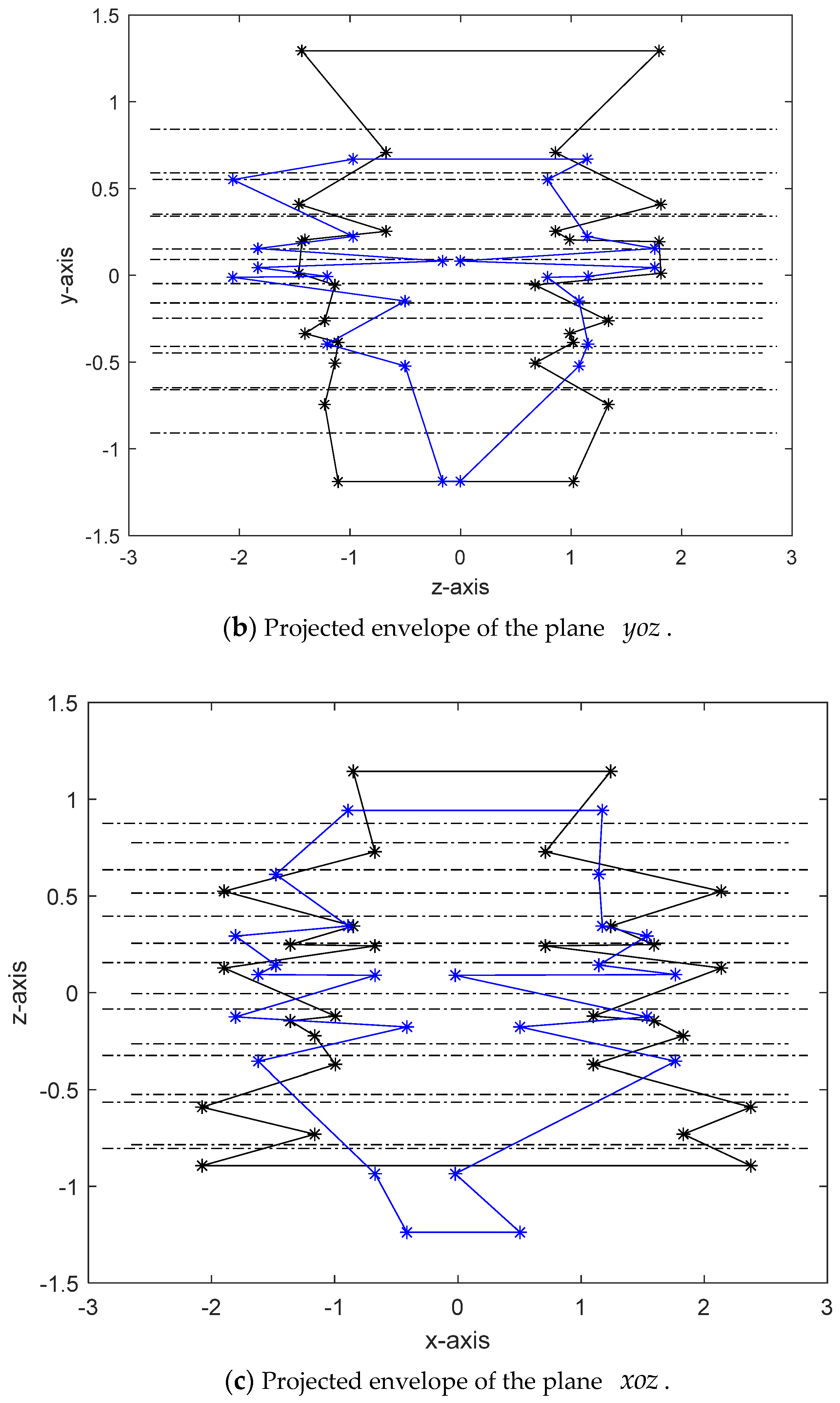
According to the above calculation method, the projection envelopes of the three, two-dimensional coordinate planes $xoy$, $yoz$, and $xoz$ of the semi-physical simulation data and the external field data are drawn and the corresponding areas are calculated, as shown in Figure 11. The black line is the semi-physical simulation data envelope polyline, the blue line is the external field data envelope polyline, and the corresponding area ratios of the planes $xoy$, $yoz$, and $xoz$ are 71.75%, 56.61%, and 79.68%, respectively. Observing the graph envelope situation shows that the integrity detection is not satisfied. The simulation data that do not satisfy the integrity detection in this example are directly fused with the field test data based on the Bayesian method, and the fusion result is shown in Figure 12.

Considering situations where the above examples do not satisfy the integrity detection conditions, a surrogate model of the semi-physical simulation system based on the BPNN method is considered, and the test conditions are supplemented. The semi-physical simulation test is repeated under the supplementary test conditions to obtain supplementary landing point data, thereby obtaining a complete semi-physical simulation landing point dataset. The envelope of the field datapoints is shown in Figure 12.

According to the test conditions corresponding to the landing point data in the calculation example, based on the BPNN method, the test conditions of the nonenveloped field landing point data are predicted. The predicted data results are shown in

Table 2. Prediction results of test conditions for the unenveloped outfield landing point coordinate data.

Test Condition	Landing Point 1	Landing Point 2	Landing Point 3	Landing Point 4	Landing Point 5
Temperature (°C)	6.422	−0.399	11.8677	−4.6979	−0.5227
Wind speed (m/s)	3.5128	3.3814	18.9298	6.0319	2.3971
Wind direction (°)	131.1504	44.7598	95.7029	3.0727	74.3106
Flight altitude (km)	7668.2	7326.7	9528.5	7811.6	6661.9
Flight speed (km/h)	884.2053	834.6266	871.7192	793.1395	850.1596
x-axis direction attitude angle (°)	17.0863	10.289	51.7779	8.2403	0.135
y-axis direction attitude angle (°)	69.74	59.7432	80.8241	58.3418	57.2935
z-axis direction attitude angle (°)	193.3593	204.1317	257.7273	229.0353	176.5477

.

According to the prediction results of the test conditions that are not enveloped, the originally set test condition range is expanded. After that, the semi-physical simulation test is carried out under the complete test conditions and the corresponding simulation data of the landing point coordinates are obtained to realize the expansion of the semi-physical simulation landing data and obtain a complete semi-physical simulation landing dataset. Based on Bayesian theory, the semi-physical simulation data in the calculation example and the field test data are fused and analyzed, and the empirical distribution function image is drawn as shown in Figure 13.

The qualitative analysis in Figure 13 shows that the empirical distribution function fused with the field test data is closer to the cumulative distribution function of the actual flight landing point of a 534A aircraft after supplementing the simulation data, which does not satisfy the completeness test as a whole. Let the CDF of the data population be $F_t^o(x)$; the EDF of the fusion after supplementation be $F_t^s(x)$; and the EDF of the directly fused data be $F_t^d(x)$. The area metrics calculated by Formula (13) are:

$$\begin{gathered} A(F_t^o(x),F_t^o(x))=0.1048;A(F_t^o(y),F_t^s(y))=0.0861;A(F_t^o(z),F_t^s(z))=0.0950 \\ A(F_t^o(x),F_t^d(x))=0.3232;A(F_t^o(y),F_t^d(y))=0.2621;A(F_t^o(z),F_t^d(z))=0.2882 \end{gathered}$$

Therefore, it is proven that the proposed method of integrity detection and supplementary test design of the semi-physical simulation data of the aircraft landing point is effective for data fusion.

7. Discussions and Conclusions

Taking the test results of the landing point coordinates of a semi-physical simulation system of an aircraft as the research object, an integrity detection criterion based on field test data and expert estimation information is established. The integrity detection of semi-physical simulation data includes four steps: ① reducing the dimensionality of the 3D landing point data; ② realizing data expansion and regularization based on a bootstrap resampling method; ③ drawing the statistical envelope of the confidence region; and ④ establishing the integrity detection criterion. Based on the BPNN method, the agent model of the semi-physical simulation system is constructed for the landing point which does not satisfy the completeness requirement, and the test conditions of the data of the landing point are supplemented.

Through the application of research in the field and semi-physical simulation tests of the aircraft 534A in Section 6, aiming at the coordinate data of the field and semi-physical simulation, integrity detection and a supplementary experimental design of the aircraft semi-physical simulation data were carried out. The result of data processing shows that after adding semi-physical simulation data that does not satisfy the integrity detection, the EDF fused with field test data is closer to the CDF of the actual landing point of aircraft 534A. It is verified that the method proposed in this paper can lay a good foundation for the data fusion of the following semi-physical simulations and field tests. This approach has a number of beneficial effects:

(1) An integrity detection method for semi-physical simulation data is creatively proposed, which can quantitatively test the completeness of simulation data for semi-physical simulation systems based on external field placement data and expert estimated envelope conditions. This effectively improves the semi-physical performance and the practical application significance of the effect and completeness assessment of the fusion of simulation data and field test data.

(2) The established test standard is applicable to data completeness measurements under large and small samples (bootstrap resampling can be used to expand the sample data).

(3) The established test standard is applicable to both the integrity detection measure of a single index and the overall completeness measure of multiple indexes of an entire system (data dimensionality reduction is sufficient) and has good generality.

At the same time, it should be noted that to fully verify the completeness of the model data, a variety of means and methods must be used and bottom-up, multi-index, layer-by-layer aggregation methods must be used for the model indicators. Only then can the final comprehensive evaluation result of the completeness of the semi-physical simulation model be obtained. In addition, this paper’s “Integrity detection and supplementary experimental design of semi-physical simulation data of aircraft landing points” not only applies to semi-physical simulation data and data processing methods. In fact, the equivalent experiment in aircraft not only includes semi-physical simulation experiments, but also includes digital simulation experiments, numerical simulation experiments, ground static simulation experiments, and so on. Whether the data processing method in this paper can be directly applied to the equivalent experimental data of other aircraft substitutions needs further study.