Author Contributions
Conceptualization, M.D. and K.L.; methodology, K.L.; software, K.L. and D.L.; investigation, K.L. and D.L.; resources, M.D.; data curation, D.L.; writing—original draft preparation, K.L.; writing—review and editing, D.L. and J.X.; visualization, K.L. and D.L; supervision, M.D.; project administration, M.D.; funding acquisition, M.D. All authors have read and agreed to the published version of the manuscript.
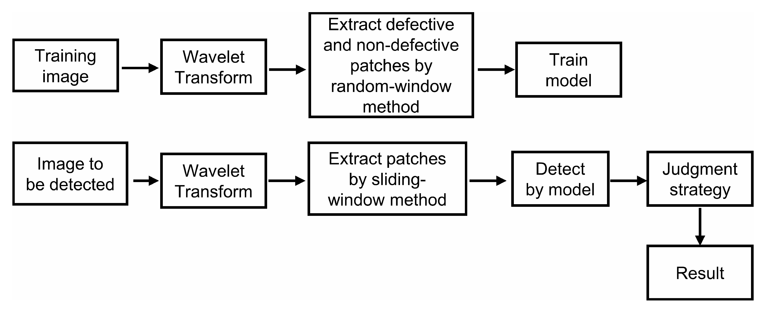
Figure 1.
The general process of this paper’s method. The wavelet-transformed images are extracted as defective and non-defective patches, respectively. Feed it into the network to train the model. When testing, use a sliding window to input the wavelet-transformed image into the model for judgment and decision-making.
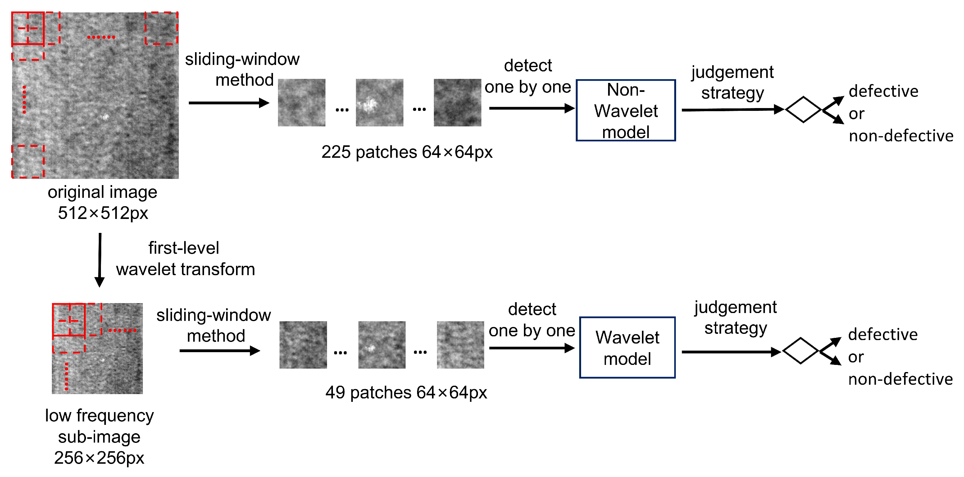
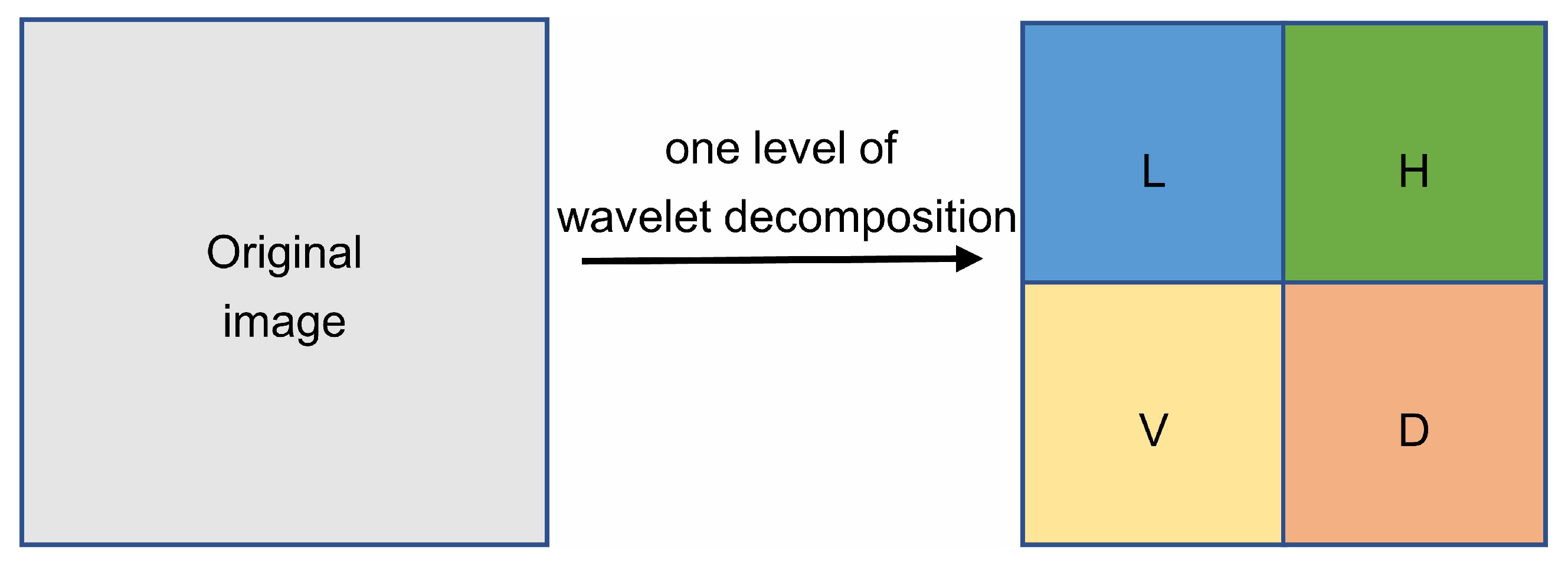
Figure 2.
One level of wavelet decomposition. L, H, V, D represent low-frequency coefficient, horizontal high-frequency coefficient, vertical high-frequency coefficient and diagonal high-frequency coefficient.
Figure 2.
One level of wavelet decomposition. L, H, V, D represent low-frequency coefficient, horizontal high-frequency coefficient, vertical high-frequency coefficient and diagonal high-frequency coefficient.
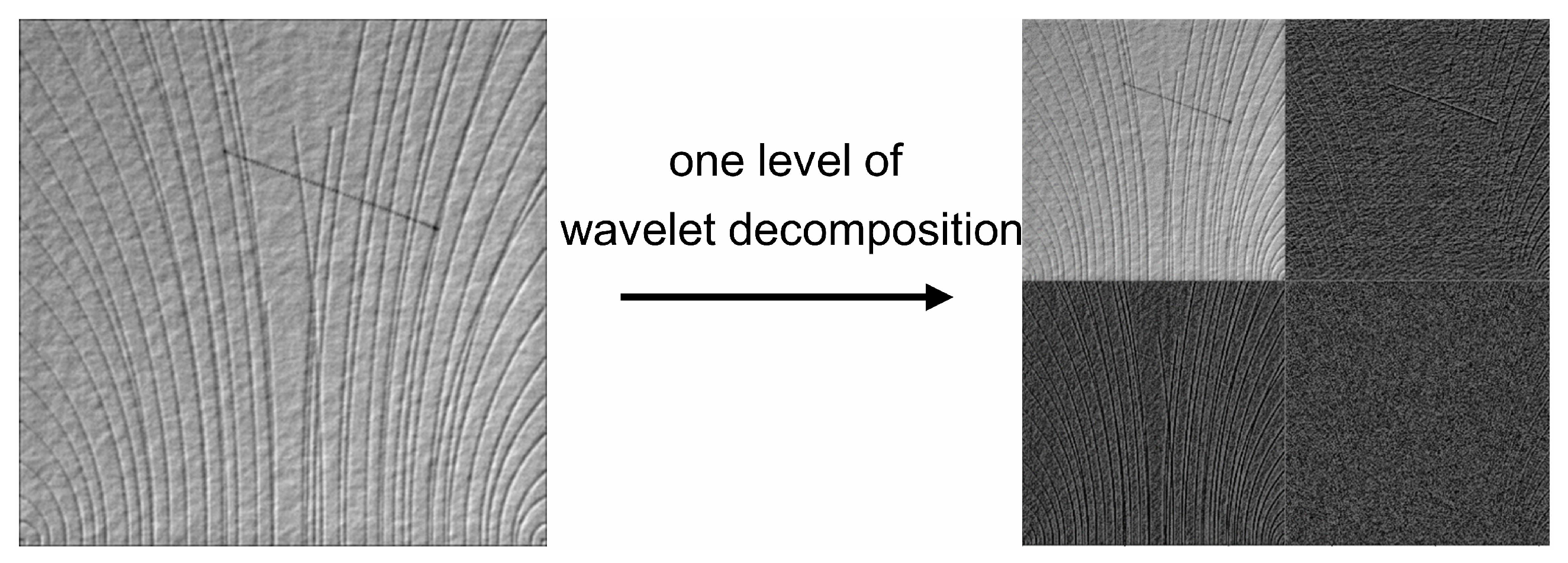
Figure 3.
The decomposition results of the real image. The right side is the decomposed four different frequency submaps.
Figure 3.
The decomposition results of the real image. The right side is the decomposed four different frequency submaps.
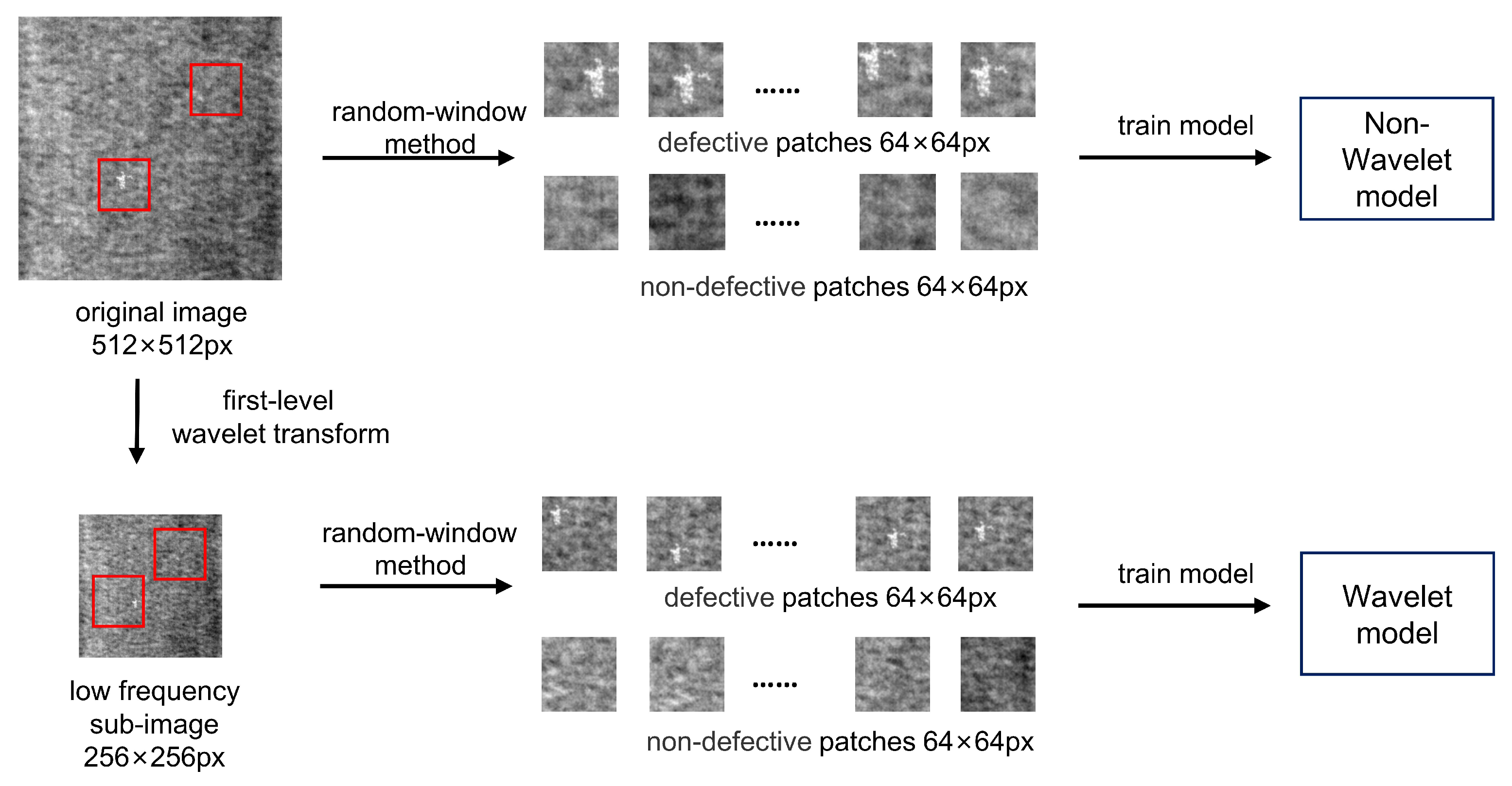
Figure 4.
The process of this method in the model training phase. The original image and wavelet image are divided into patches and sent to the network for training respectively.
Figure 4.
The process of this method in the model training phase. The original image and wavelet image are divided into patches and sent to the network for training respectively.
Figure 5.
Into patches and then sent to the two models for judgment.
Figure 5.
Into patches and then sent to the two models for judgment.
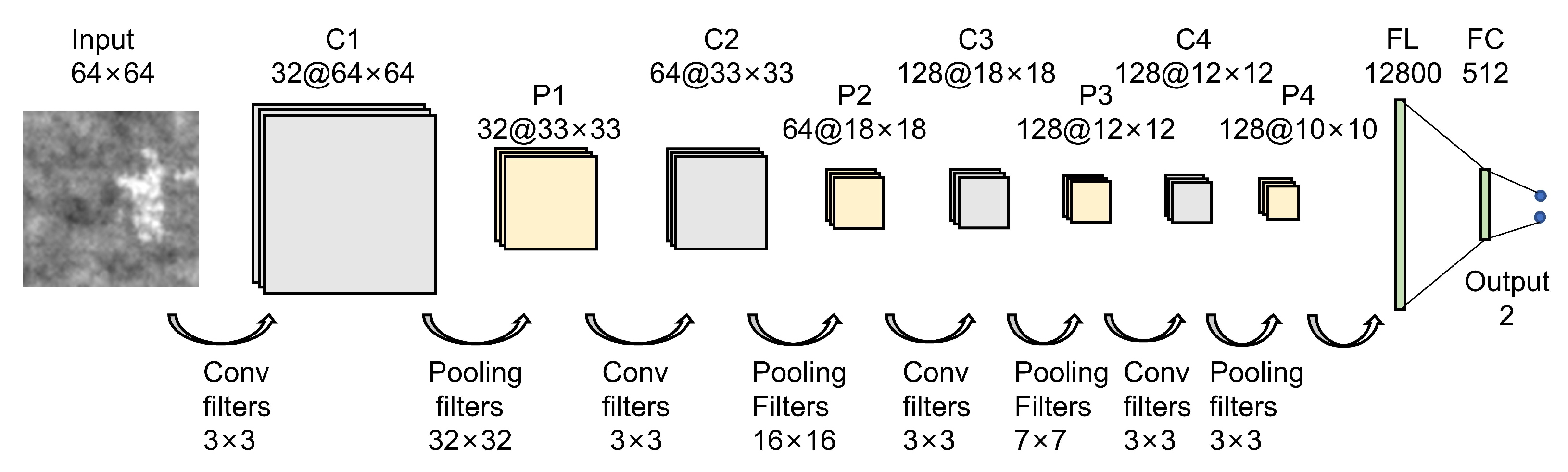
Figure 6.
The architecture of our CNN networks for defect detection.
Figure 6.
The architecture of our CNN networks for defect detection.
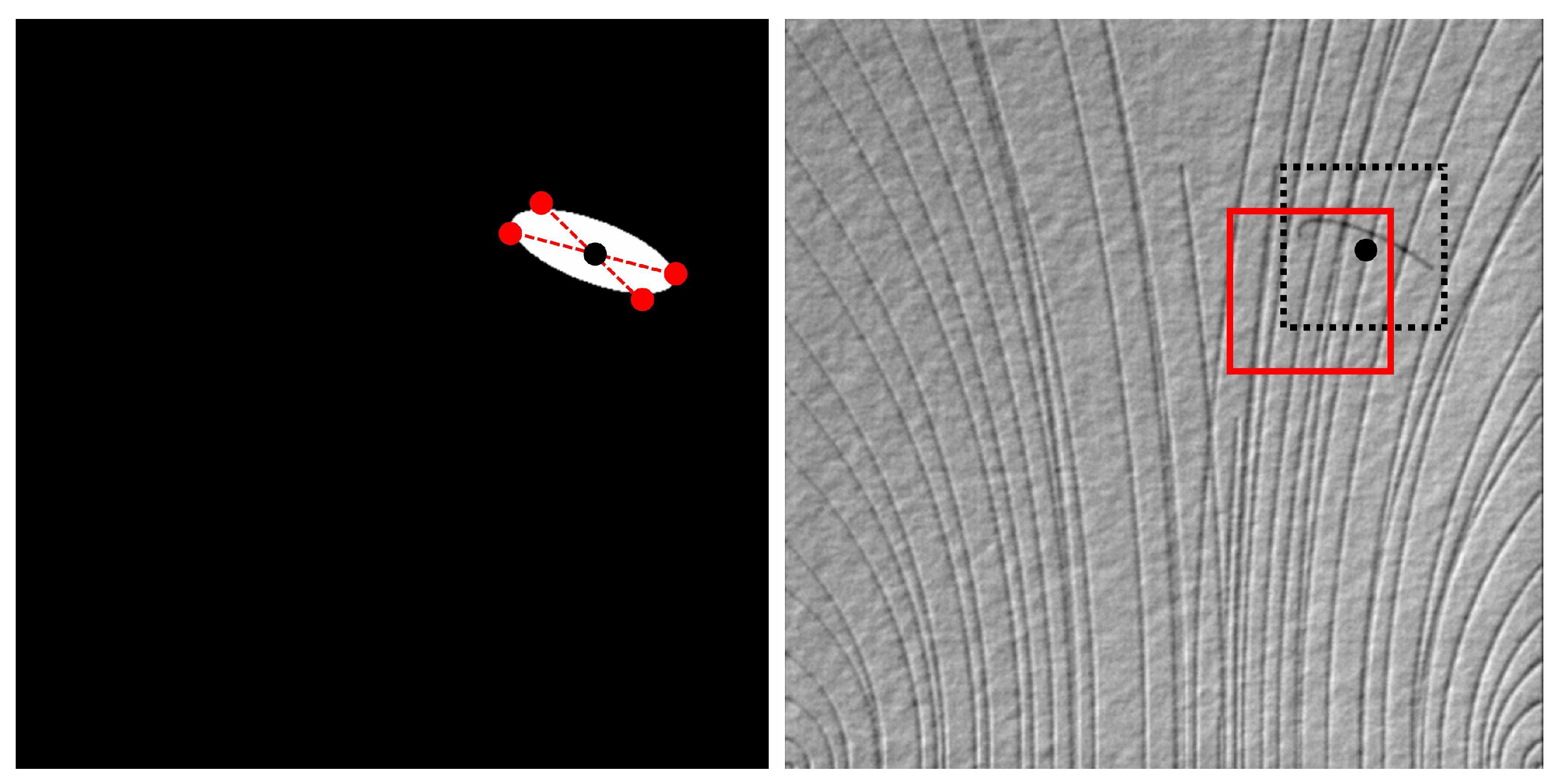
Figure 7.
Label image (left) and defect image (right) in DAGM. The black spot is the center of the defect, the red rectangle is the defect patch we extracted after offset.
Figure 7.
Label image (left) and defect image (right) in DAGM. The black spot is the center of the defect, the red rectangle is the defect patch we extracted after offset.
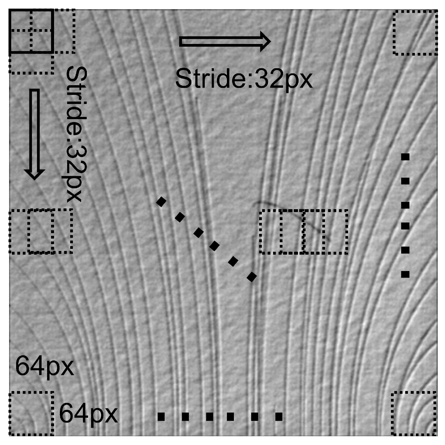
Figure 8.
The sliding-window method in DAGM 2007. Extract all 64 × 64 patches in the image in 32 strides for prediction.
Figure 8.
The sliding-window method in DAGM 2007. Extract all 64 × 64 patches in the image in 32 strides for prediction.
Figure 9.
A defective image (right) and its probability matrix (left). The number in the box indicates the probability that the patch is non-defective.
Figure 9.
A defective image (right) and its probability matrix (left). The number in the box indicates the probability that the patch is non-defective.
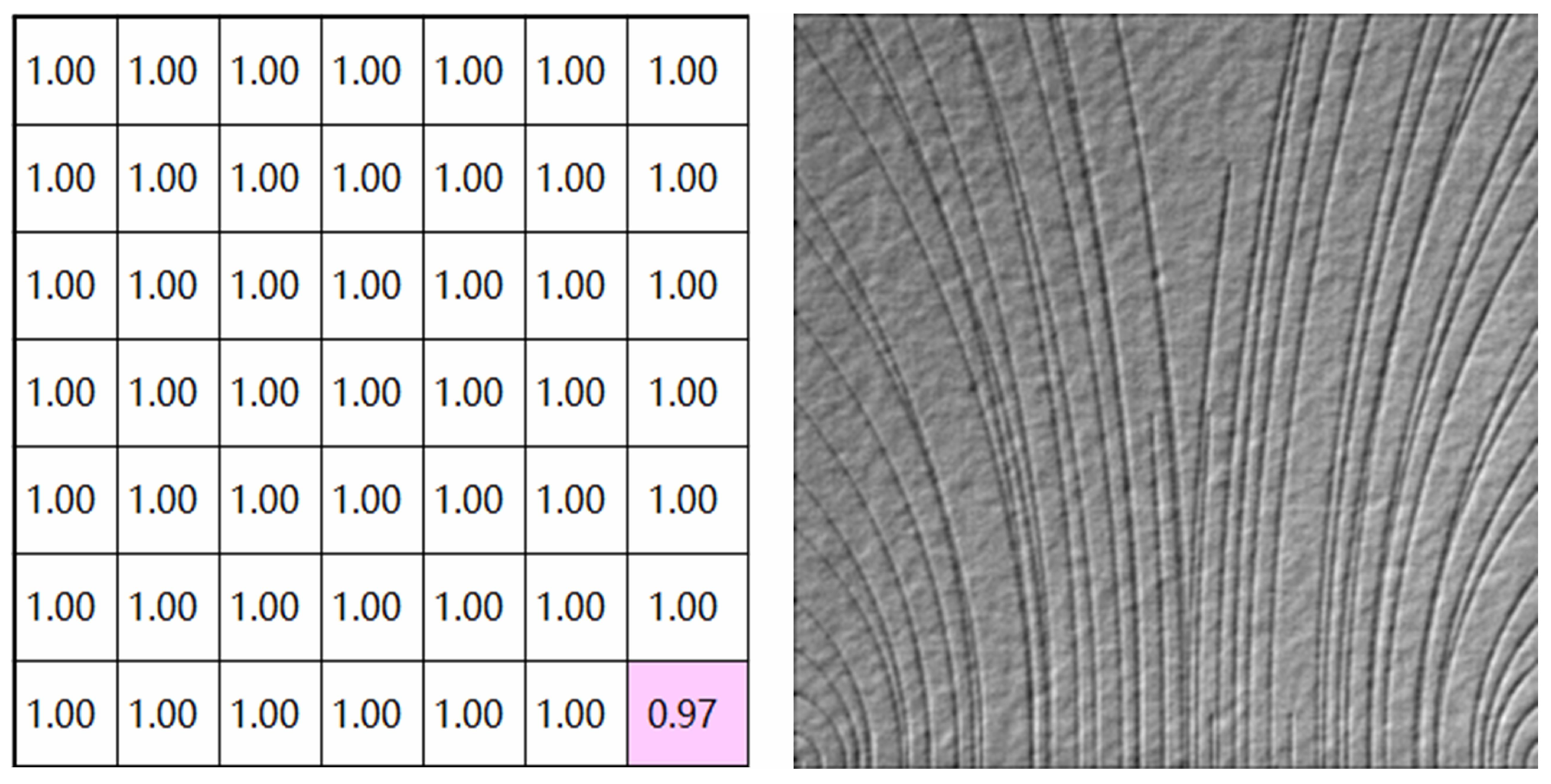
Figure 10.
A non-defective image (right) and its probability matrix (left). The number in the box indicates the probability that the patch is non-defective.
Figure 10.
A non-defective image (right) and its probability matrix (left). The number in the box indicates the probability that the patch is non-defective.
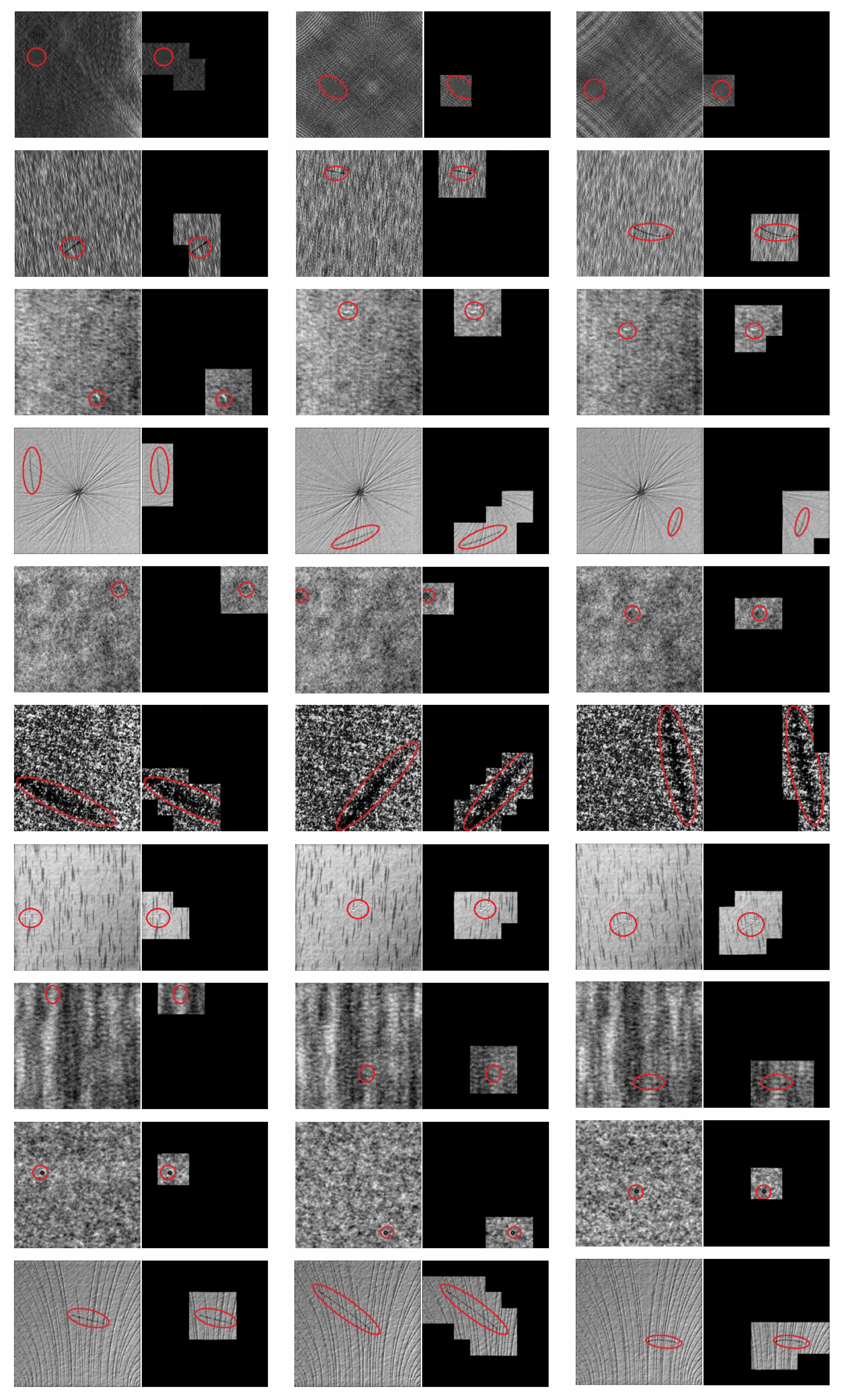
Figure 11.
The image samples of 10 classes in DAGM2007 dataset. Defects are marked with red ellipses.
Figure 11.
The image samples of 10 classes in DAGM2007 dataset. Defects are marked with red ellipses.
Figure 12.
The image samples of two classes in the micro-surface defect database. Defects are marked with red ellipses.
Figure 12.
The image samples of two classes in the micro-surface defect database. Defects are marked with red ellipses.
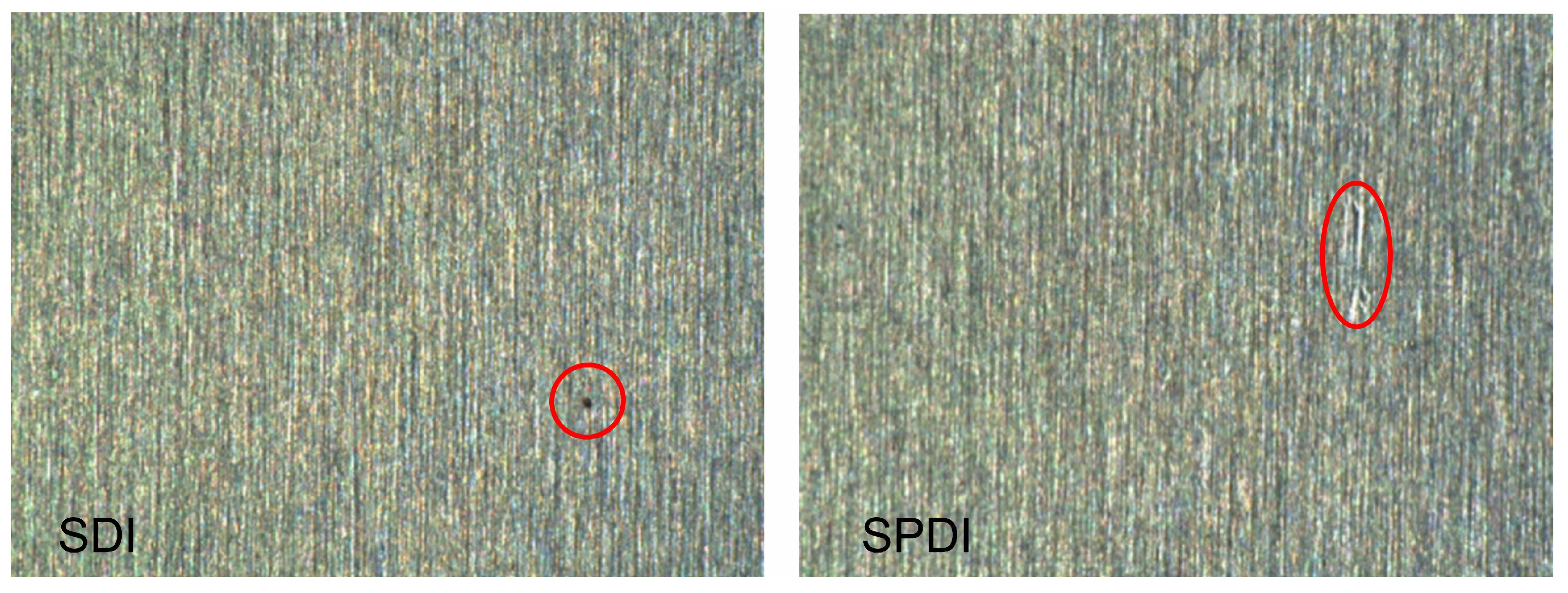
Figure 13.
The image samples in the KolektorSDD dataset. Defects are marked with red ellipses.
Figure 13.
The image samples in the KolektorSDD dataset. Defects are marked with red ellipses.
Figure 14.
The examples of detection results in the DAGM2007 dataset. The red ellipse marks the location of the defect. The left image is the image to be detected, and the right image is the detection result. Our model judges that areas without defects are covered with black images.
Figure 14.
The examples of detection results in the DAGM2007 dataset. The red ellipse marks the location of the defect. The left image is the image to be detected, and the right image is the detection result. Our model judges that areas without defects are covered with black images.
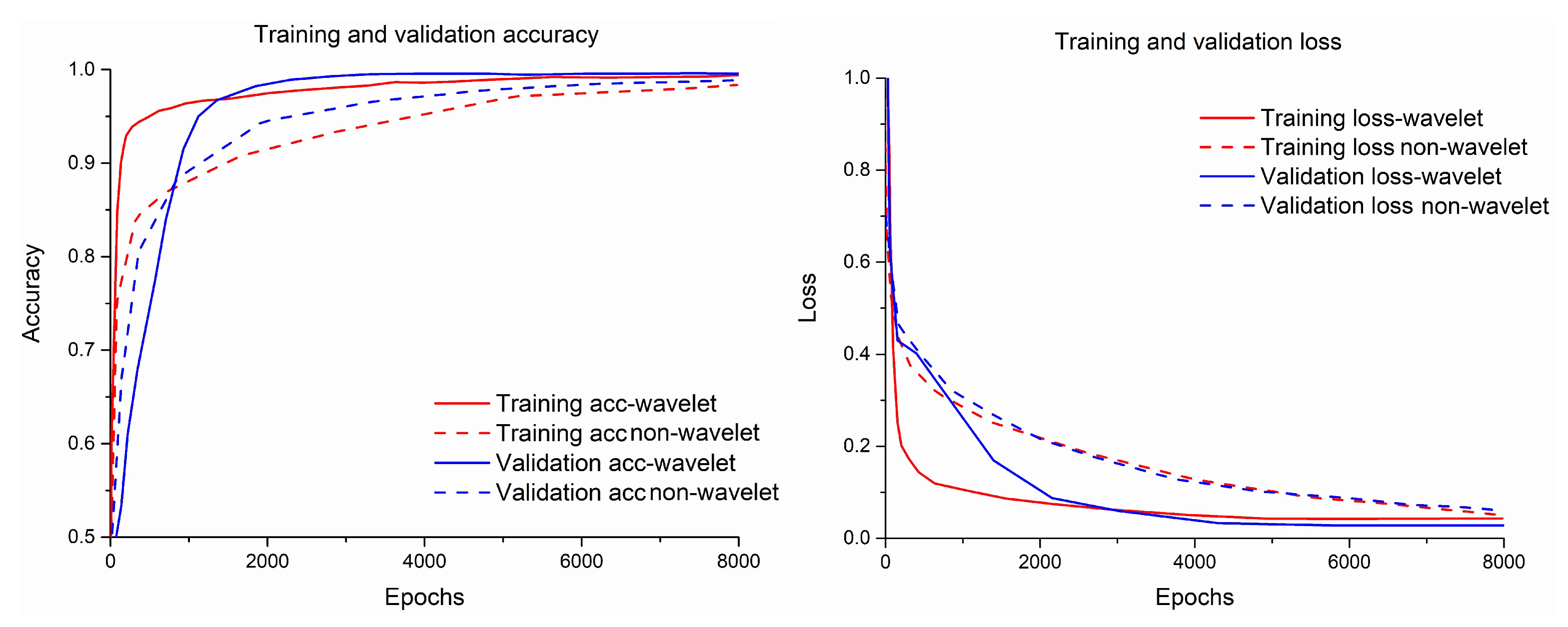
Figure 15.
The accuracy curve and loss curve of the wavelet model and non-wavelet model.
Figure 15.
The accuracy curve and loss curve of the wavelet model and non-wavelet model.
Figure 16.
The examples of detection results in a micro-surface defect database. The red ellipse marks the location of the defect. The left image is the image to be detected, and the right image is the detection result. Our model judges that areas without defects are covered with black images.
Figure 16.
The examples of detection results in a micro-surface defect database. The red ellipse marks the location of the defect. The left image is the image to be detected, and the right image is the detection result. Our model judges that areas without defects are covered with black images.
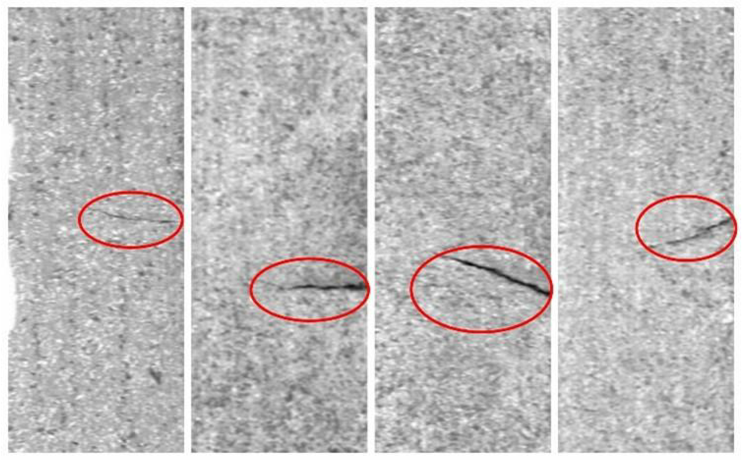
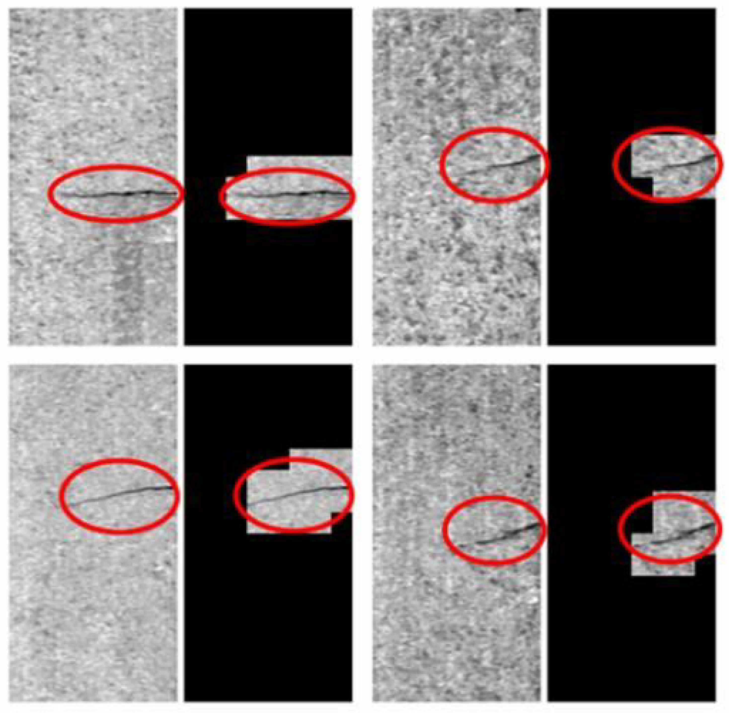
Figure 17.
The examples of detection results in the KolektorSDD dataset. The red ellipse marks the location of the defect. The left image is the image to be detected, and the right image is the detection result. Our model judges that areas without defects are covered with black images.
Figure 17.
The examples of detection results in the KolektorSDD dataset. The red ellipse marks the location of the defect. The left image is the image to be detected, and the right image is the detection result. Our model judges that areas without defects are covered with black images.
Table 1.
The image distribution of each class.
Table 1.
The image distribution of each class.
| Class | Class2 | Class3 | Class6 | Class7 | Class8 | Class9 | Class10 | Total |
|---|
| Train(P/N) 1 | 120/970 | 100/800 | 100/800 | 200/1800 | 200/800 | 200/1800 | 200/1800 | 1120/9770 |
| Test(P/N) 1 | 30/30 | 50/200 | 50/200 | 100/200 | 100/200 | 100/200 | 100/200 | 530/1230 |
Table 2.
The number of training patches of each class in the wavelet model.
Table 2.
The number of training patches of each class in the wavelet model.
| Class | Class2 | Class3 | Class6 | Class7 | Class8 | Class9 | Class10 | Total |
|---|
| Defective patches | 1503 | 1758 | 2370 | 3690 | 2814 | 2930 | 4504 | 19,589 |
| Non-defective patches | 3880 | 3200 | 2400 | 7200 | 7200 | 6000 | 5400 | 35,280 |
Table 3.
The results of our methods in the DAGM2007 dataset and the comparison of others. Here, TPR and TNR are recorded by adjusting the threshold of the judgment strategy to make the acc maximum.
Table 3.
The results of our methods in the DAGM2007 dataset and the comparison of others. Here, TPR and TNR are recorded by adjusting the threshold of the judgment strategy to make the acc maximum.
| Class | Our Non-Wavelet Model | Our Wavelet Mode | Xie’s Model [25] | Racki’s CNN [1] | Wang’s CNN [2] | Weimer’s CNN [3] | Statistical Features [42] | SIFT and ANN [43] | Weibull [44] | Zhang’s Model [26] |
|---|
| TPR (%) | | | | | | | | | | |
| 2 | 95.8 | 97.5 | 100 | 100 | 100 | 100 | 94.3 | 95.7 | - * | 92.5 |
| 3 | 87.0 | 100 | 100 | 100 | 100 | 95.5 | 99.5 | 98.5 | 99.8 | 89.6 |
| 6 | 100 | 99 | 100 | 100 | 100 | 100 | 100 | 99.8 | 94.9 | 93.8 |
| 7 | 66.5 | 97.5 | 100 | 100 | - | - | - | - | - | 95.9 |
| 8 | 100 | 96.5 | 100 | 100 | - | - | - | - | - | 95.9 |
| 9 | 74 | 99.5 | 100 | 100 | - | - | - | - | - | - |
| 10 | 51 | 92 | 100 | 100 | - | - | - | - | - | - |
| TNR (%) | | | | | | | | | | |
| 2 | 97.5 | 99.4 | 100 | 99.8 | 100 | 97.3 | 80 | 91.3 | - | - |
| 3 | 98.8 | 99 | 100 | 96.3 | 100 | 100 | 100 | 100 | 100 | - |
| 6 | 100 | 99.9 | 100 | 100 | 100 | 99.5 | 96.1 | 100 | 100 | - |
| 7 | 100 | 99.5 | 100 | 100 | - | - | - | - | - | - |
| 8 | 100 | 98.9 | 100 | 100 | - | - | - | - | - | - |
| 9 | 95.9 | 100 | 100 | 99.9 | - | - | - | - | - | - |
| 10 | 99.9 | 99.8 | 100 | 100 | - | - | - | - | - | - |
| AVEACC (%) | | | | | | | | | | |
| | 96.1 | 99.3 | 100 | 99.7 | 99.8 | 99.2 | 95.9 | 98.2 | 97.1 | - |
Table 4.
The number of pixels in each training set between our method and others.
Table 4.
The number of pixels in each training set between our method and others.
| Class | Our Wavelet Model | Racki’s CNN [1] | Wang’s CNN [2] | Weimer’S CNN [3] |
|---|
| Class1–6 | 20,631,552 px | 209,190,912 px | 867,631,104 px | 221,729,792 px |
| | (5037 × 64 × 64) * | (798 × 512 × 512) | (52,956 × 128 × 128) | (216,533 × 32 × 32) |
| Class7–10 | 40,710,144 px | 419,430,400 px | - | - |
| | (9939 × 64 × 64) | (1600 × 512 × 512) | - | - |
| Ratio | 1 | 10.24 | 42.05 | 10.75 |
| AVEACC (%) | 99.3 | 99.7 | 99.8 | 99.2 |
Table 5.
The performance criteria of detecting SDI and SDPI.
Table 5.
The performance criteria of detecting SDI and SDPI.
| Class | TP | FP | FN | Recall (%) | Precession (%) |
|---|
| SDI * | 24 | 0 | 2 | 92.3 | 100 |
| SDPI * | 24 | 1 | 1 | 96 | 96 |
Table 6.
The performance criteria of detecting the KolektorSDD dataset.
Table 6.
The performance criteria of detecting the KolektorSDD dataset.
| TP | FP | FN | Recall (%) | Precession (%) |
|---|
| 16 | 0 | 4 | 80 | 100 |


