Effect of Air Inlet Spacing on Air Distribution and Ventilation Performance of Stratum Ventilation Using Multiple Parallel Jets

Abstract

An appropriate layout of air terminals can improve the thermal comfort and air quality for room occupants. Stratum ventilation (SV) can efficiently provide thermal comfort and quality of inhaled air. However, investigations into the impact of the supply air inlet spacing on performance under SV are lacking. This study conducted experimental measurements and numerical simulations to analyze the effect of the supply inlet spacing on the air distribution and ventilation performance of the SV. Six theoretical axial velocity attenuation formulas were verified using experimental results. The effective draft temperature for SV (EDTS), air diffusion performance index (ADPI), the local mean age of air (LMAA), and energy utilization coefficient (EUC) were used as the evaluation indexes. The results indicated that the modified Abramovich formula was the most suitable for predicting the attenuation of the axial velocity of multiple parallel jets under SV. At an air supply spacing of 650 mm, the position near the central air supply inlet experienced a cold thermal environment with high air velocity and low air temperature; the positions on both sides of the room were warmer owing to insufficient airflow. The air distribution at these positions improved with increasing air inlet spacing, but some areas could not be covered by the supply airflow. The optimal value of ADPI corresponded to an air inlet spacing of 800 mm, whereas optimal LMAA and EUC corresponded to a spacing of 950 mm. Analysis of a multi-objective optimization method indicated that an air inlet spacing of 800 mm provided optimal overall performance.

1. Introduction

Energy consumption is one of the most important factors to be considered in the design of new buildings, which is also an index that the existing buildings need to improve [1]. Recent research has shown that the energy consumption of commercial and residential buildings is responsible for approximately 40% of the total energy consumption [2]. The amount of energy used in heating, ventilation, and air-conditioning (HVAC) systems accounts for almost half of the energy consumption in buildings [3]. The energy consumed is primarily used to create a healthy and comfortable indoor environment [4]. Reducing energy consumption while meeting indoor environmental requirements is important in mitigating carbon emissions. Considering that people spend more than 80% of their time indoors [5], an environment with poor indoor air quality can cause diseases such as sick building syndrome [6], which can seriously affect the health of occupants [7]. Since the COVID-19 pandemic, with aerosol transmission as a main route of transmission, indoor air quality has become a focus of attention. In an indoor environment, ventilation can effectively mitigate airborne transmission risk in confined spaces [8]. Thus, optimizing the ventilation control method [9] and using advanced air distribution [10,11] were considered to improve the ventilation efficiency in this study.

As air distribution advances [12], stratum ventilation (SV) is an excellent potential solution for both substantial energy savings and air quality [13]. The conditioned clean air is supplied directly to the breathing zone through air inlets installed at the mid-level on the side walls [14], which shortens the supply air path. The thermal neutral temperature of SV is approximately 27 °C, 2.5 °C higher than that of mixing ventilation, and 2.0 °C higher than that of displacement ventilation [15]. The energy savings of SV were found to be at least 44% and 25% per year compared to mixing ventilation and displacement ventilation, respectively [16]. Experimental results indicate that SV can provide satisfactory overall and local thermal comfort at a room temperature of 27 °C [15,17], with small vertical air temperature differences between the head and foot [18]. SV can also provide good air quality [18]. Tian et al. [19] investigated gaseous contaminant diffusion under SV and found that the concentration along the supply air jet was lower than in other parts of the room. Recent studies have been conducted to improve the performance and increase the application of SV. Zhang et al. [20] proposed a subzone control method for SV to improve thermal comfort. Compared with the conventional method, the advanced method reduced the deviation between the PMV (predicted mean vote of thermal sensation) in the subzone and the preferred one by 17.6–41.5%. A robust thermal deviation evaluation method was proposed for the design optimization of air distribution [21]. The robustly optimized constant air volume system of SV increased thermal comfort by 8.5% compared with one of the variable air volume systems. Cheng et al. [17] conducted a subjective study in an environment room with SV to evaluate the effects of temperature and supply air velocity on thermal comfort. Experimental and computational fluid dynamics (CFD) simulation studies have validated the feasibility of SV in multirow rooms [22]. Wu et al. [23] considered a walking occupant in typical offices and found the application potential with frequently walking occupants compared to traditional ventilation methods. Studies have reported that SV performance is affected by the design parameters. Yao et al. [24] conducted experiments and found that exhaust location and supply airflow rate can affect air diffusion. Fong et al. [25] studied four exhaust types for SV, and the results indicated that rear-middle-level-exhausted SV can satisfy human comfort needs with the least energy consumption.

As the supply air inlets of SV are horizontally arranged on the same wall, multiple parallel jets interact with each other during delivery to the occupied zone, which directly affects indoor air distribution. Based on numerical simulations, Zheng et al. [26] found that jet spacing has an important impact on jet interaction, which decreases with an increase in jet spacing. The merge point between parallel jets varies significantly with the change in jet spacing. Yin et al. [27] conducted an experimental study on twin jet flow generated by two identical parallel axisymmetric nozzles. The results showed that the turbulence energy increased when the Reynolds number increased. A high Reynolds number indicates a strong mutual attraction between the twin jets. Liu et al. [28] conducted a theoretical analysis and experimental studies and found a similarity criterion between two and three parallel jets. In addition, researchers have found that the characteristics of twin parallel jets are influenced by the ratio of nozzle axis spacing d to nozzle width w (nozzle spacing ratio, d/w). Wang and Tan [29] demonstrated the periodic interaction between twin jets owing to the existence of a Carmen vortex at d/w = 1. Mondal et al. [30] found that the peak value of jet velocity decreased with an increase in the nozzle spacing ratio at 0.6 ≤ d/w ≤ 1.4. Liu et al. [31] studied rectangular nozzles and found that the nozzle spacing ratio and merging point exhibited consistent trends. For SV, multiple identical air inlets are often arranged in parallel on the side wall of the room; interaction between the jets due to the influence of the jet spacing cannot be neglected.

Recent studies have focused mainly on the effects of the supply air temperature, supply air angle, and air terminal type. Research on the influence of parallel jet spacing on SV performance is lacking. Air inlet spacing of SV directly affects the air jet interaction and air distribution, affecting thermal comfort and inhaled air quality. If the parallel jet spacing is too small, multiple air jets enter the occupied zone after merging with insufficient airflow diffusion. A large parallel jet spacing results in an occupied zone that cannot be fully covered by the supply air. Thus, this study innovatively investigates the effect of air inlet spacing on the flow characteristics and ventilation performance of SV using multiple parallel jets. Experiments and computational fluid dynamics (CFD) simulations were conducted. The effective draft temperature for SV (EDTS), air diffusion performance index (ADPI), the local mean age of air (LMAA), and energy utilization coefficient (EUC) were used to comprehensively evaluate the ventilation performance. The six theoretical axial velocity attenuation formulas were adopted, and the predicted results were compared with the experimental results. The optimal air inlet spacing was obtained using the TOPSIS multi-objective optimization method. The research results enrich the understanding of airflow characteristics and optimization of SV design.

2. Methodology

2.1. Experimental Method

2.1.1. Experimental Platform

All experiments were performed in the environment chamber of a laboratory at Chongqing University, as shown in Figure 1. The environment chamber was designed to investigate multiple ventilation methods, including stratum ventilation, mixing ventilation, deflection ventilation, and displacement ventilation. The chamber dimensions are 5040 mm (length) × 5850 mm (width) × 2550 mm (height). The walls and windows of the laboratory are internal envelope enclosures. The left and right walls contain windows with areas of 4.3 m² and 1.4 m², respectively. Eight cuboid manikins with dimensions of 400 mm × 250 mm × 1200 mm were arranged in the occupied zone to simulate sedentary occupants [32]. A 100 W light bulb was installed inside each manikin to simulate the heat dissipation of the body [33]. Six 23 W fluorescent lamps were placed on the ceiling.

Different ventilation methods can be realized by switching the valves of different ducts. Yao and Lin [24] found that when the layout of SV air inlets and exhaust outlets meets the following requirements, it is conducive to better air mixing in the occupied zone, effectively improving indoor air quality: the air inlets and exhaust outlets are located on the same side, and exhaust outlets are located in the lower part of the room. Thus, this arrangement was used for the experiments. Three double-deflection grille diffusers and three exhaust outlets were installed on the same front wall. The dimensions of all terminals were 180 mm × 180 mm. The lower edges of the air inlet and exhaust outlet were located at heights of approximately 1220 mm and 330 mm above the floor, respectively. The spacing between two adjacent terminals was adjusted by opening or closing the air inlets.

2.1.2. Experimental Cases

To analyze the influence of the spacing between supply air inlets on the indoor thermal environment in the occupied zone, supply air velocities of 1.21 m/s and 1.62 m/s, and air inlet spacings of 650 mm and 1300 mm were used, as presented in

Table 1. Experimental conditions.

Test Series	Case	V0 (m/s)	L (mm)
	1	1.21	650
Series 1	2	1.62
	3	1.21	1300
	4	1.62
	5	1.53	650
Series 2	6	2.02	650
	7	2.02	1300

Note: V₀ = supply air velocity; L = air inlet spacing.

(Series 1). Cases 1 and 3, and Cases 2 and 4 with the same supply air velocity were designed to explore the effects of different air inlet spacings. As the supply air of SV diffuses directly to the heads of the occupants, the air temperature in the occupied zone should be controlled within a certain range to avoid affecting the thermal comfort of the occupants. The average measured air temperature in the occupied zone was around 27.0 °C in Cases 1 and 3, and around 27.2 °C in Cases 2 and 4. In these four cases, the average air temperature met the SV thermal neutral temperature of the room of 27 °C [13]. In Series 2, Cases 5–7 had supply air velocities of 1.53 m/s and 2.02 m/s, and air inlet spacings of 650 mm and 1300 mm to verify six theoretical axial velocity attenuation formulas for three parallel air inlets.

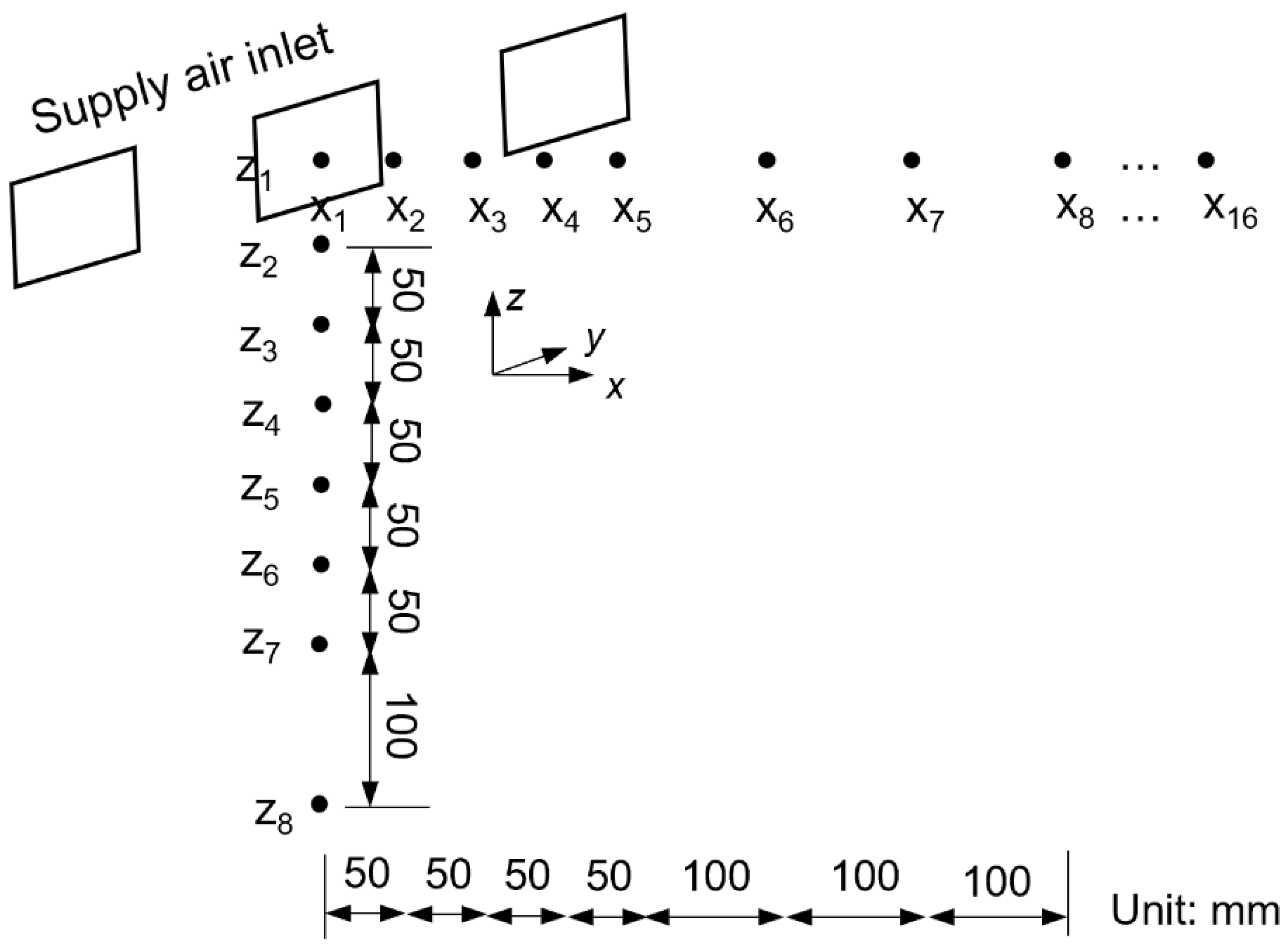
2.1.3. Experimental Measurements

To obtain the distributions of temperature and velocity in the occupied zone, four sampling lines (Lines 1–4) were arranged in the occupied zone, as shown in Figure 1b. Each sampling line contained four measurement points at heights of 0.1 m, 0.6 m, 1.1 m, and 1.7 m above the floor. In addition, the change in the axial velocity of the jet was represented by the value of the air velocities at the measurement points, which were arranged horizontally and vertically on the jet center plane, as shown in Figure 2. The velocity change in the initial section of the jet was more obvious; thus, the measurement points near the center of the middle air inlet needed to be more concentrated; 128 measurement points were distributed in eight rows and 16 columns.

To ensure the airtightness of the envelopes, the cracks in doors, windows, and temporarily unused air inlets were sealed. All measurement instruments were calibrated prior to the experiments. The average room air temperature is calculated by the value of three measurement points distributed at a height of 1.1 m in the occupied zone. Detailed information on the measurement instruments is listed in

Table 2. Information on the measurement instruments.

Instrument		Measuring Location	Parameter	Range	Accuracy	Sampling Frequency
WZY-1		Room air	Temperature	−20–80 °C	±0.3 °C	0.2 Hz
		Envelope	Temperature			0.003 Hz
Swema 03+		Supply air and all the measurement points in the occupied zone and jet area	Velocity	0.05–10 m/s	±0.03 m/s ± 3%	8 Hz
			Temperature	10–40 °C	±0.2 °C

. In this study, only data recorded in a steady environment were used. The frequency conversion fan and air handling unit were turned on about one hour before the experiments. A steady indoor environment was identified by stationary air temperature monitored using Swema 03+. During the measurement, the sampling lines were measured separately owing to the limitations of the instruments. Collection of air velocities and temperatures along one sampling line lasted 6 min. The instruments were then manually moved to the next sampling line slightly. To minimize the disturbance of movement, the data of the next sampling line were not recorded until Swema 03+ displayed a stable environment again. The interval between two adjacent data collections was at least 10 min.

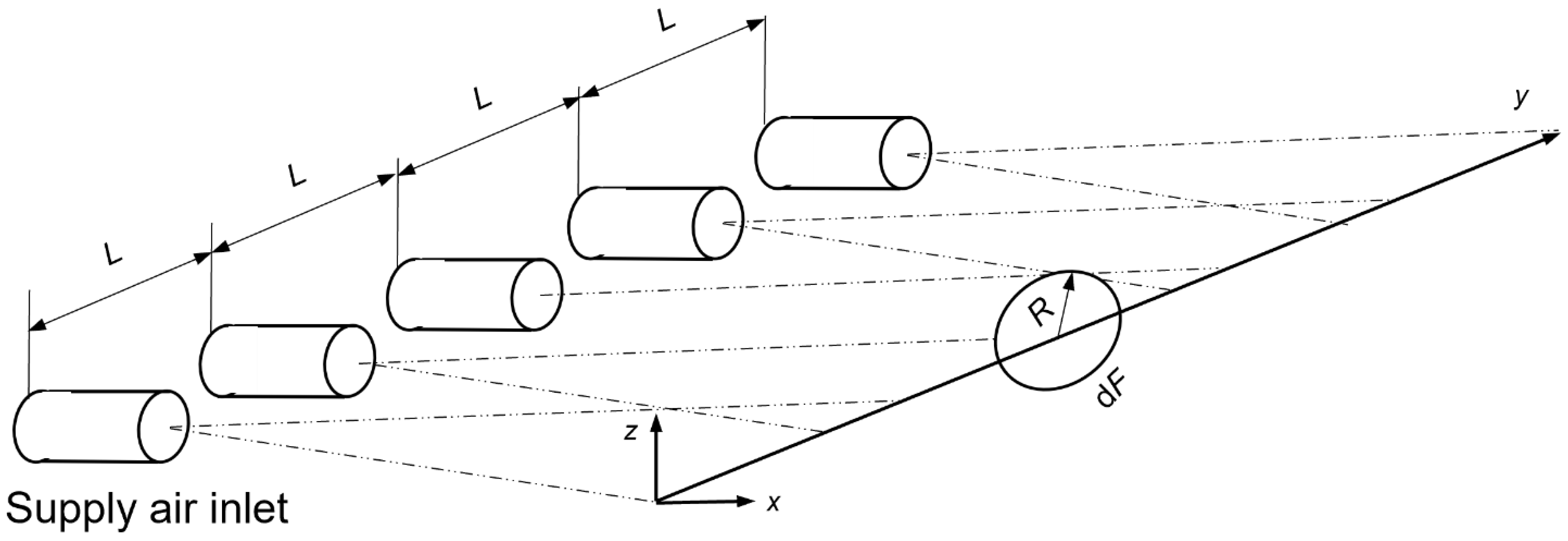
2.2. Theory of Multiple Parallel Jets

The jet interaction with multiple jets arranged in parallel is shown in Figure 3. The spacing between the air inlets is L, and the air inlets have the same diameter and supply air volume. The momentum of the jet from each air supply inlet is P_i (i = 1, 2, 3 …, n). It is assumed that the infinitesimal area vertical to the cross-section of the jet is dF. The radius of the infinitesimal area is R. According to the law of conservation of momentum [34], the momentum on the cross-section is the sum of the momentum of all jets flowing through the cross-sectional area.

$$\begin{array}{c}dP=d{P}_1+d{P}_2+d{P}_3+\cdots \cdots +d{P}_{\mathrm{n}}\end{array}$$

(1)

where

$$\begin{array}{c}dP=\rho v^{2}dF,d{P}_1={\rho }_1{v}_1^{2}dF,\cdots \cdots ,d{P}_n={\rho }_n{v}_n^{2}dF\end{array}$$

(2)

where $v_1,v_2,\cdots ,v_n$ is the average velocity of each jet passing through the section (m/s); ${\rho }_1,{\rho }_2,\cdots ,{\rho }_n$ is the density of each single jet (kg/m³); $v$ is the velocity at the study point (m/s).

The air densities at each supply air inlet can be regarded as equal. The equation can be simplified as

$$\begin{array}{c}{v}^2=v_1^2+v_2^2+\cdots \cdots +v_n^2={\displaystyle \sum _{i=1}^n}{v}_i^2\end{array}$$

(3)

According to the sectional velocity of a single jet proposed by Shapelev [35], the equation is defined as

$$\begin{array}{c}\frac{v_r}{v_c}=\exp \left[-\frac{1}{2}{\left(\frac{r}{cx}\right)}^2\right]\end{array}$$

(4)

where $v_c$ is the axial velocity of the single jet at x from the supply air inlet (m/s), $r$ is the distance from the study point to the axis of the single jet (m), $v_r$ is the velocity at a distance $r$ from the axis coordinate $x$ (m/s), c is a constant (0.082 in this study).

On the premise of uniform supply air at each supply air inlet of the SV, the axial air velocity of each jet can be considered to be the same. The equation can be deduced as

$$\begin{array}{c}v=v_x\sqrt{{\displaystyle \sum _{i=1}^n}\mathrm{e}\mathrm{x}\mathrm{p}\left[-{\left(\frac{r_i}{0.082x}\right)}^2\right]}=K_v·v_x\end{array}$$

(5)

where

$$\begin{array}{c}{K}_v=\sqrt{{\displaystyle \sum _{i=1}^n}\mathrm{e}\mathrm{x}\mathrm{p}\left(-{\left(\frac{r_i}{0.082x}\right)}^2\right)}\end{array}$$

(6)

Overlapping correction coefficient of velocity $K_v$ was established on a Shapelev normal distribution. As three equally spaced supply air inlets were arranged in the experiment, the velocity attenuation formula of the axis of the central air outlet can be expressed as

$$\begin{array}{c}v=k_v·v_x=\sqrt{2\mathrm{e}\mathrm{x}\mathrm{p}\left[-{\left(\frac{L}{0.082x}\right)}^2\right]}·v_x\end{array}$$

(7)

There are many semi-empirical attenuation formulas for the axial velocity $v_x$ at different downstream distances in previous studies. Zhou [36] obtained the following formula for calculating the axial velocity attenuation of multiple parallel jets:

$$\begin{array}{c}\frac{v_x}{v_0}=3.347A_r^{-0.147}{\left(\frac{x}{d_0}\right)}^{-1.151}\end{array}$$

(8)

where $Ar$ is the Archimedes number, and $d_0$ is the diameter of the nozzle (m).

Abramovich [37] obtained the formula through dimensional analysis:

$$\begin{array}{c}\frac{v_x}{v_0}=\frac{0.48}{\frac{ax}{d_0}+0.145}\end{array}$$

(9)

where $a$ is a turbulence coefficient affected by nozzle type.

The modified formula is obtained by neglecting the short distance from the intersection point to the edge of the air inlet:

$$\begin{array}{c}\frac{v_x}{v_0}=\frac{1.13\times 0.48\sqrt{F_0}}{ax}\end{array}$$

(10)

where $F_0$ is the area of the air inlet (m²).

Alfred Koestel [38] obtained the axial velocity attenuation formula:

$$\begin{array}{c}\frac{v_x}{v_0}=1.13k_1\frac{\sqrt{F_0}}{x}\end{array}$$

(11)

Li [39] derived unified formulas for an air jet, buoyant plume, and buoyant jet:

$$\begin{array}{c}\frac{v_x}{v_0}=3.5{\left\{6.41{\frac{x}{d_0}}^{-3}+{Ar}^{\frac{2}{3}}{\frac{x}{d_0}}^{-1}\right\}}^{\frac{1}{3}}\end{array}$$

(12)

Bahalev [37] proposed an inductive solution based on a model experiment:

$$\begin{array}{c}\frac{v_x}{v_0}=\left(6.5-4.5e^{-0.5\frac{x}{d_0}}\right){\left(2+\frac{x}{d_0}\right)}^{-1}{e}^{-0.001\frac{x}{d_0}}\end{array}$$

(13)

Equations (8)–(13) are substituted into Equation (7) to obtain $V_1$–$V_6$, which are analyzed in Section 3.2.1.

2.3. Numerical Simulation

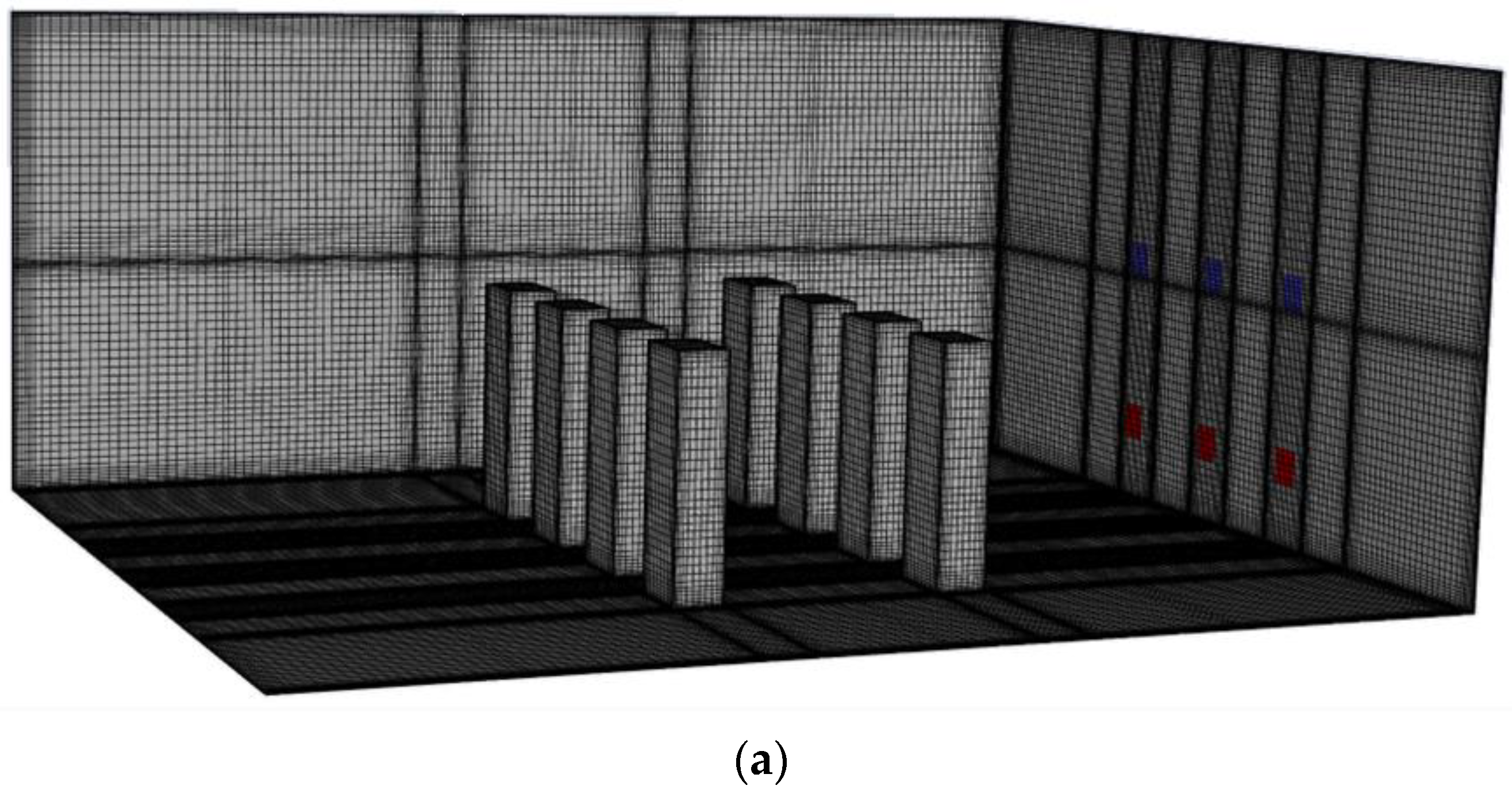
2.3.1. CFD Model

CFD has been widely recognized as an independent research method due to its low cost compared with experimental measurements [40,41]. In this study, a CFD model based on the commercial program FLUENT was used to perform the simulation, which was validated by experimental measurements. The built model was based on the environment chamber used in the experiments, as shown in Figure 4. The room layout and geometric dimensions of the CFD model were identical to those of the chamber.

Appropriate boundary conditions are essential to ensure the accuracy of the CFD numerical simulation results. The supply air inlets and exhaust outlets were set as the velocity inlet boundary and outflow boundary conditions, respectively. The indoor heat sources, including thermal manikins and ceiling lamps, were set as constant heat flux boundary conditions. The envelope was defined as a constant wall temperature. The expression of the governing equations and the boundary condition settings for the numerical simulations are presented in

Table 3. Governing equations.

Governing Equations	$\mathbf{\varnothing }$	${{\Gamma }}_{\mathbf{\varnothing }}$	${\mathit{S}}_{\mathbf{\varnothing }}$
Mass equation	1	0	0
Momentum equation	$u_i$	$\mu +{\mu }_i$	${-\partial }_p/{\partial }_x-\rho g_i\beta (T-T_0)$
Energy equation	T	$\mu /P_r+{\mu }_t/{\sigma }_t$	$S_T$
Turbulent kinetic energy equation	k	$\mu +{\mu }_t/{\sigma }_k$	$G_k+G_b-\rho \epsilon -Y_M$
Turbulent dissipation equation	$\epsilon$	$\mu +{\mu }_t/{\sigma }_{\epsilon }$	$C_{1\epsilon }(G_k+C_{3\epsilon }{G}_b)/k-C_{2\epsilon }\rho {\epsilon }^2/k+S_{\epsilon }$

and

Table 4. Boundary conditions for simulation calculation.

Boundary	Boundary Condition
Supply air inlet	Velocity inlet
Exhaust outlet	Outflow
Window, walls, and ceiling	Constant wall temperature, 28.4 °C
Floor	Constant wall temperature, 27.2 °C
Occupant	Constant heat flux, 60.24 W/m2
Light	Constant heat flux, 638.89 W/m2

, respectively.

The standard k-ε, RNG k-ε, and SST k-ω models perform well in predicting the distributions of air velocity and temperature, according to previous studies [42]. The standard k-ε and RNG k-ε models used the standard wall function. The SST k-ω model solved throughout the near-wall flows [43]. In this study, the prediction accuracies of the three turbulence models were compared, and the model with the highest accuracy was used for the next simulation calculation. The discrete ordinate (DO) model was used to calculate the heat transfer between different wall surfaces (walls, windows, human body surfaces, and lamps). The Boussinesq model was used to consider the buoyancy effect [44]. A second-order upwind scheme was used to discretize the momentum, energy, and turbulence equations. SIMPLE was used as the pressure–velocity coupling method. The energy-scaled residuals and radiation intensity residuals were set to 1 × 10⁻⁶, and the other scale residuals were set to 1 × 10⁻⁴.

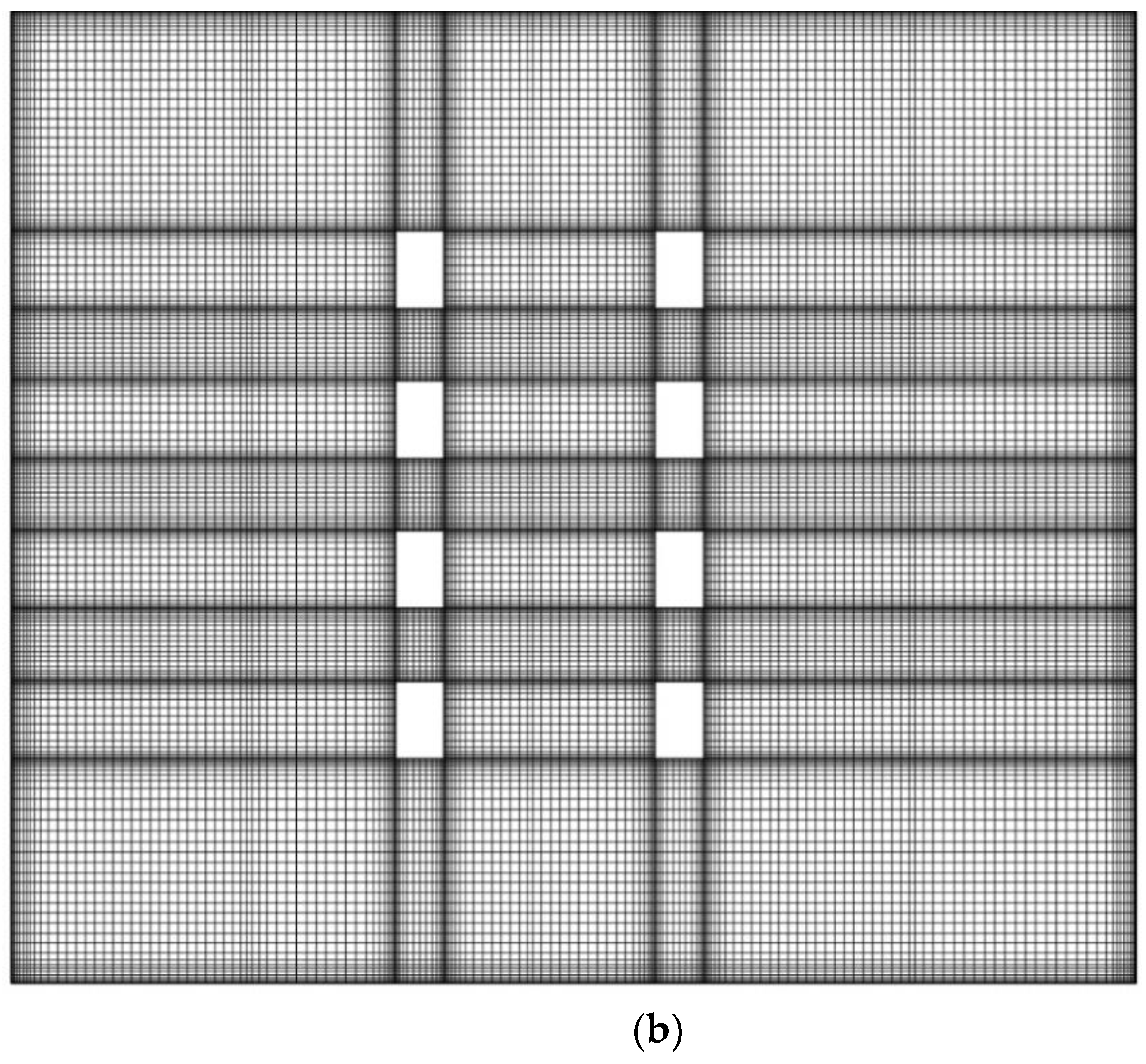
2.3.2. Grid Independence Tests

The ICEM was used to mesh the model with structured grids, which consumed less time and increased the accuracy of the calculation compared to unstructured grids. In addition, the grids near the supply air inlet, exhaust outlet, and the area around the occupants were refined. The grids are shown in Figure 5. The height of the first layer of the grid was determined according to the non-dimensional wall distance (y⁺) [45].

For the grid-independence tests, CFD models with 1,110,000 (coarse), 2,600,000 (moderate), and 3,110,000 (fine) hexahedron grids were selected. With air velocity, temperature, and air inlet spacing of 1.62 m/s, 22.8 °C, and 650 mm, the temperature and velocity along Sampling Line 1 were compared for the three grids, as shown in Figure 6. It was found that when the grid was changed from moderate to fine, the differences in velocity and temperature were insignificant, whereas the differences between the moderate and coarse grids were large. Thus, the moderate grid was used considering both the prediction accuracy and calculation cost.

2.3.3. Studied Cases

The average room temperature with a supply air velocity of 1.5 m/s and supply air temperature of 23.5 °C was the closest to the thermal neutral temperature of approximately 27 °C under SV. Thus, the simulation cases were designed as shown in

Table 5. Simulated cases.

Case	T0 (°C)	V0 (m/s)	L (mm)
1	23.5	1.5	500
2			650
3			800
4			950
5			1100
6			1250

Note: T₀ = supply air temperature; V₀ = supply air velocity; L = air inlet spacing.

based on the supply air condition. Various air inlet spacings were designed to explore their effect on the air distribution and ventilation performance of the SV using multiple parallel jets.

2.3.4. Evaluation Indices

To evaluate the SV performance, the following evaluation indices were used:

• Effective draft temperature for SV (EDTS);
• Air diffusion performance index (ADPI);
• Local mean age of air (LMAA);
• Energy utilization coefficient (EUC).

In addition to the widely used PMV model [46], the EDTS index is also frequently used for evaluating SV. It was proposed by Lin [47] and was found to be reliable for evaluating thermal comfort of SV. When −1.2 K < EDTS < 1.2 K, the thermal comfort is evaluated as satisfactory. EDTS was calculated using Equation (14).

$$\begin{array}{c}EDTS=\left(t_x-t_{room}\right)-\left(v_x-1.1\right)\end{array}$$

(14)

where $t_x$ is the local air temperature (°C), $t_{room}$ is the average room temperature (°C), and $v_x$ is the local air velocity (m/s).

The ADPI was used to assess the uniformity of air velocity and temperature distributions and their contribution to thermal comfort [48]. The more comfortable the thermal environment, the larger is the ADPI. The ADPI was calculated using Equation (15).

$$\begin{array}{c}ADPI=\frac{n_i\left(-1.2K < EDTS < 1.2K, 0 < v < 0.8m/s\right)}{n}\end{array}$$

(15)

where n represents the number of nodes in the occupied zone [49], and n_i represents the number of nodes when the EDTS of the nodes is in the comfort range.

The local mean age of air was defined as the average time between air particles entering a room to arriving at a certain point indoors. It is an effective index for measuring the freshness of indoor air and is widely used in evaluating the indoor air quality of buildings [50]. The smaller the air age, the higher the air freshness. It can be solved as an additional transport scalar; the transport equation is [38]

$$\begin{array}{c}\frac{\partial }{\partial \mathrm{t}}\left(\rho \tau \right)+\frac{\partial }{\partial x_j}\left(\rho u_j\tau \right)=\frac{\partial }{\partial x_j}\left({\mathrm{\Gamma }}_{\tau }\frac{\partial \tau }{\partial x_j}\right)+S_0\end{array}$$

(16)

where $\tau$ is the local mean air age (s) of all micro-masses at that point, ${\mathrm{\Gamma }}_{\tau }$ is the diffusion coefficient, and $S_0$ is the source term.

The energy utilization efficiency can be quantified by comparing the air temperature in the occupied zone and the exhaust air temperature. A larger EUC value indicates a better energy-saving effect. The EUC was calculated using Equation (17).

$$\begin{array}{c}{\epsilon }_t=\frac{T_p-T_s}{T_o-T_s}\end{array}$$

(17)

where $T_p$ represents the exhaust air temperature (°C), $T_s$ represents the supply air temperature (°C), and $T_o$ represents the average temperature in the occupied zone (°C).

3. Results and Discussion

The error analysis for the measurements of air temperature and velocity were conducted. The relative uncertainty is given by:

$$\begin{array}{c}\frac{\Delta R}{R}={\left[{\sum }_{i=1}^n{(\Delta X_i/X_i)}^2\right]}^{1/2}\end{array}$$

(18)

where $R$ represents the measured variant; $\Delta R$ represents the uncertainty; $X_i$ represents independent variable and $\Delta X_i$ represents the uncertainty of $X_i$. For the WZY-1 and Swema 03+ used in this study, the measurement uncertainties for the temperature were found to be 0.3% and 0.7%, respectively. The uncertainty of Swema 03+ for the air velocity was 0.3%.

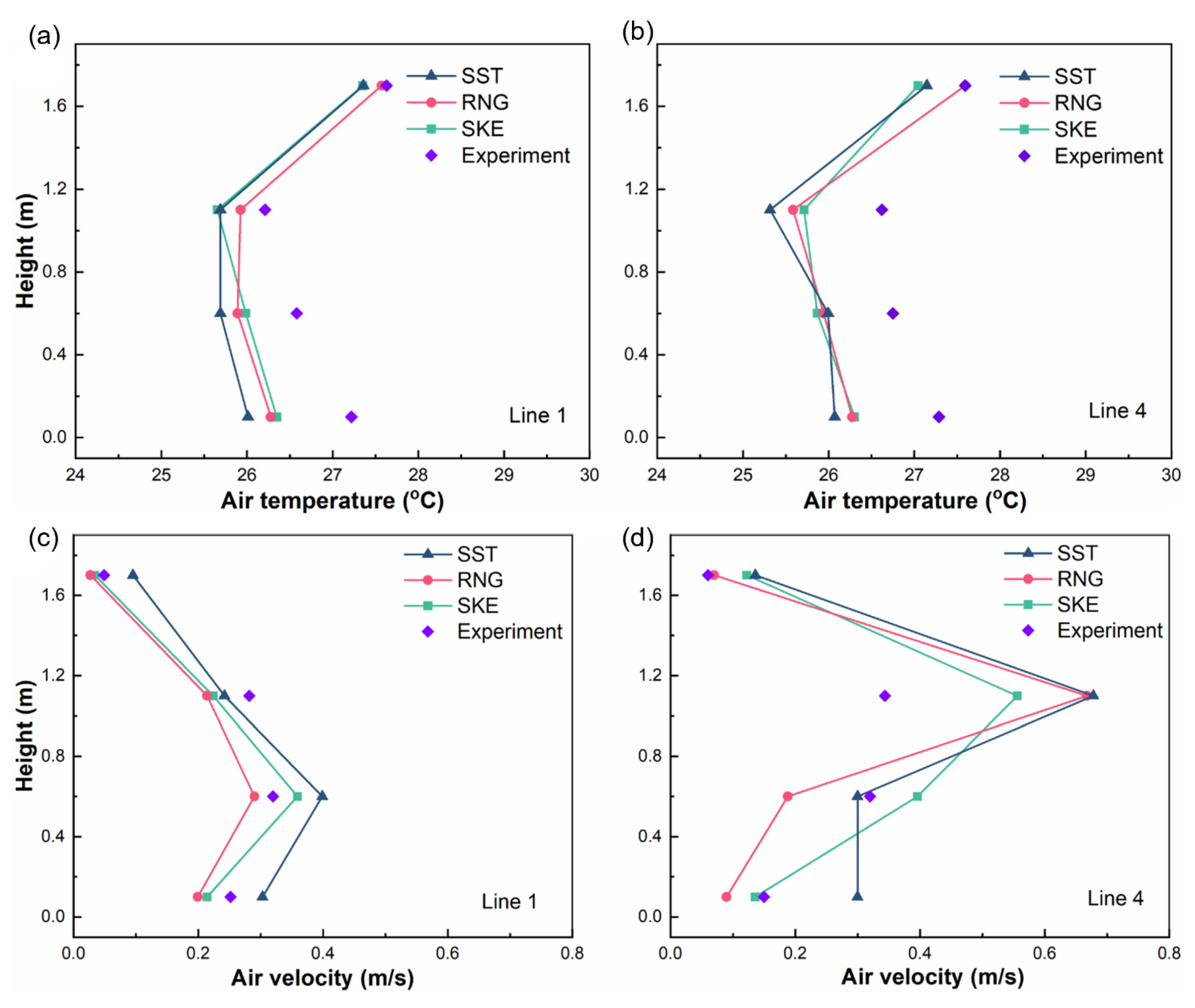
3.1. Validation of Numerical Model

To ensure the reliability of the numerical simulation, the CFD model was validated using the air velocity and temperature measured by the sampling lines in the environmental chamber. Detailed results are shown in Figure 7. Comparing the temperature and velocity predicted by three turbulence models with the experimental results along Sampling Lines 1 and 4 with supply air conditions of 1.62 m/s and 22.8 °C and an air inlet spacing of 650 mm, the simulation results were all close to the experimental results. With an increase in the height of the measurement point from the floor, the temperature of the measurement points along Line 1 and Line 4 decreased slowly, reached a minimum at a height of 1.1 m, and then increased rapidly. The temperature of both sampling lines at a height of 1.7 m exceeded 27 °C. The air velocity at the measurement point exhibited the opposite trend as the height increased. The peak value of air velocity along Line 1 and Line 4 appeared at heights of 0.6 m and 1.1 m, respectively.

The root mean square error (RMSE) of the three numerical simulation results was calculated to quantitatively analyze the consistency between the predicted and experimental results. The calculation equation is

$$\begin{array}{c}\mathrm{R}\mathrm{M}\mathrm{S}\mathrm{E}=\sqrt{\frac{1}{n}{\sum }_{j=1}^n(P_j-Q_j{)}^2}\end{array}$$

(19)

where $P_j$ is the simulation value (temperature or velocity) of the corresponding point, $Q_j$ is the measured value of the measurement point, $n$ is the number of measurement points.

The calculation results are presented in

Table 6. RMSE of velocities and temperatures in different turbulence models.

Turbulence Model	RMSE for Temperature	RMSE for Velocity
SKE	0.72	0.107
RNG	0.81	0.142
SST	0.86	0.326

. Compared with the RNG and SST models, the RMSE of temperature and velocity between the results obtained by the SKE model and experiments was the smallest, 0.72 °C and 0.107 m/s, respectively. Thus, the SKE model was selected to optimize the supply air inlet spacing of the SV. Previous studies have also shown that the SKE model has good accuracy, numerical stability, and calculation efficiency for predicting indoor airflow [51]. In a simulation study of a typical office with SV, the SKE model performed slightly better than the RNG model [52].

3.2. Experimental Results

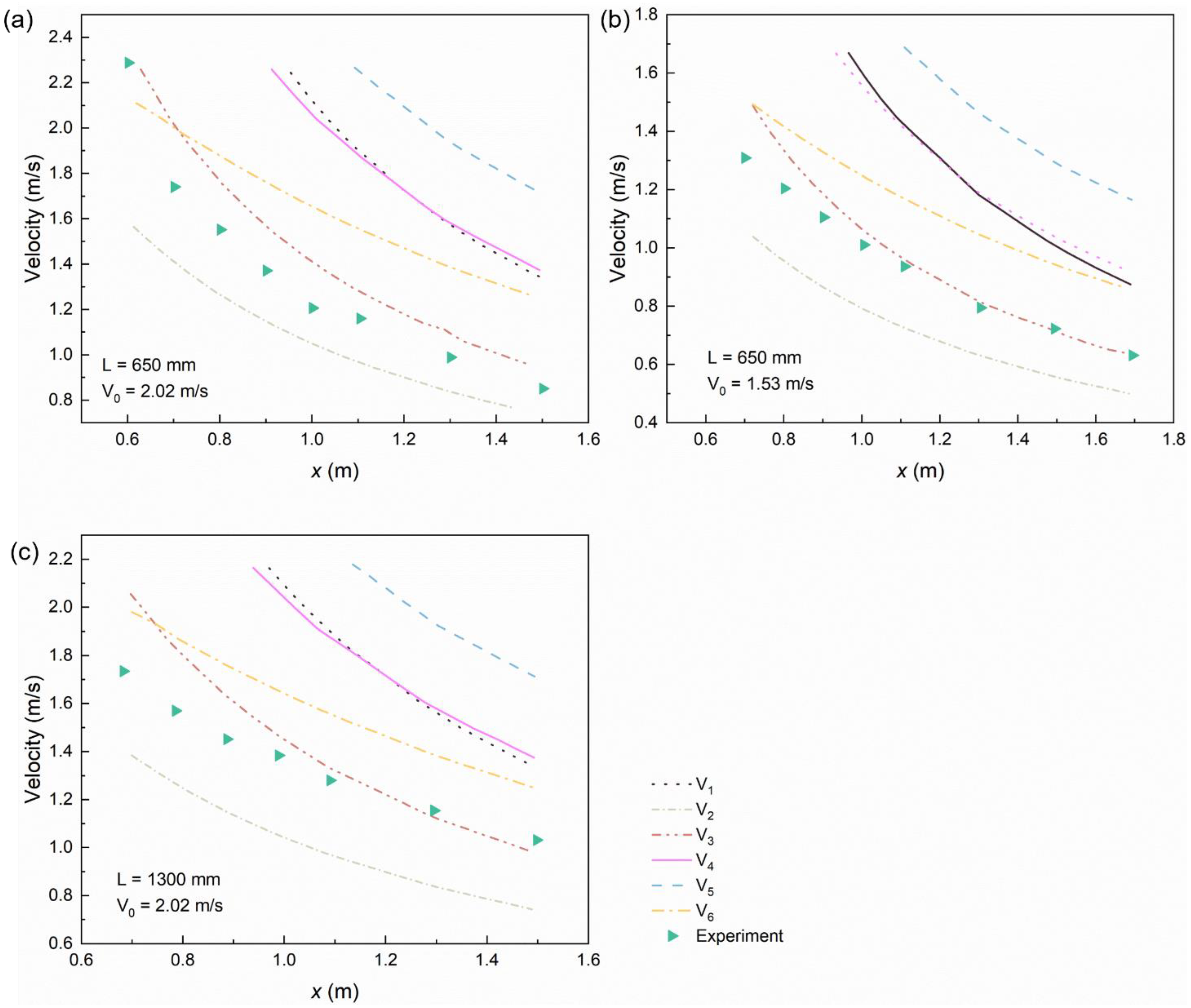
3.2.1. Verification of Theoretical Models of Multiple Parallel Jets

Equations (8)–(13) were substituted into Equation (7) to obtain $V_1$–$V_6$. In the fully developed jet zone, seven or eight typical measurement points were selected from the experimental data and compared with the results predicted by the theoretical model, as shown in Figure 8. The velocity predicted by the theoretical models was greater than the measured velocity, except $V_2$ predicted by the Abramovich theoretical model, which was lower than the measured data. Of the theoretical models, $V_5$ had the largest deviation. However, the variation trend of $V_5$ was consistent with the measured data. With a continuous increase in the outflow distance of the jet, the central velocity of the jet gradually decreased. Comparing the results, it was found that the axial velocity attenuation of $V_3$ was closest to the measured data for the three cases; the prediction curve fit the best of the six theoretical models. The RMSE between the measured data and the value of $V_3$ in the three cases was 0.23 m/s, 0.09 m/s, and 0.18 m/s, respectively. Thus, the modified Abramovich formula was the most suitable for attenuation of the axial velocity of multiple parallel jets in SV rooms.

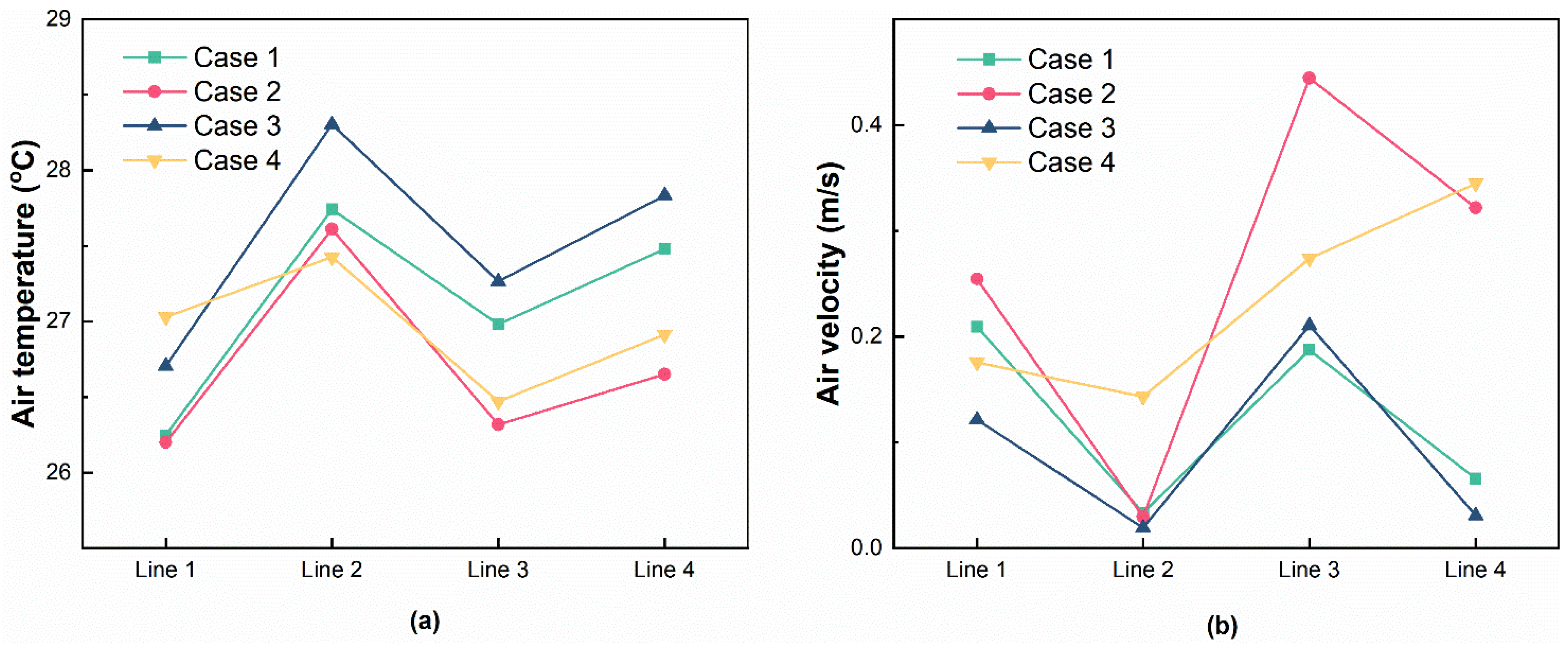
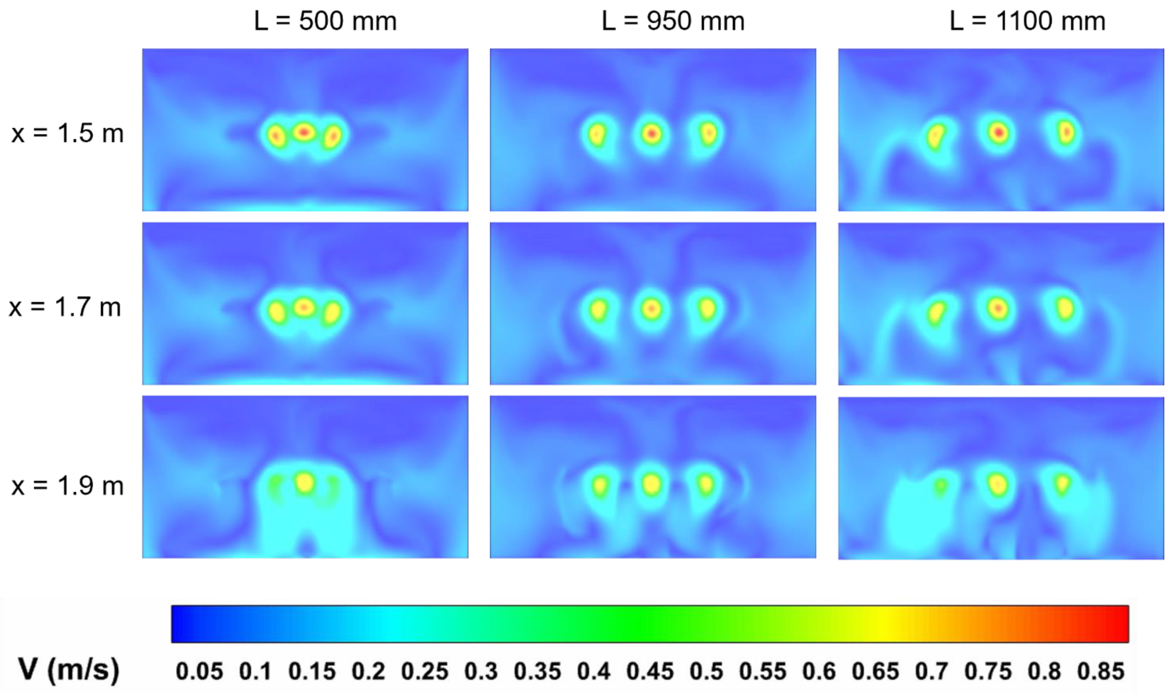
3.2.2. Influence of Air Inlet Spacing on Airflow Pattern

Figure 9 compares the air temperatures and velocities in four sampling lines at 1.1 m above the floor for the four experimental cases. The difference in the air distribution in the occupied zone at L = 650 mm and 1300 mm can be analyzed. First, the air temperatures at the measurement point of Line 1 in Case 1 were lower than those in Case 3, indicating that a smaller space between the air inlets was beneficial for cooling in the middle of the room. The air velocity at the measurement point of Line 1 in Case 1 was higher than that in Case 3, indicating that the airflow at this position was stronger with a smaller air inlet spacing. A similar phenomenon was observed in the comparison of Cases 2 and 4. The small inlet spacing caused an earlier and more concentrated confluence between the adjacent jets, which made the measurement point of Line 1 near the air inlet at the front of the room more susceptible to the impact of the jet. Second, the differences in air velocity at the measurement points of Lines 2–4 between Cases 1 and 3 were insignificant owing to the blocking effect of the occupants. However, the air temperature at the measurement points of Lines 2–4 in Case 1 was generally lower than that in Case 3, mainly due to the more concentrated jet overlapping with a small spacing. For Line 2, the air velocity was less affected by the air inlet spacing because the measuring point was located at the rear of the room, far from the air inlet. Similar air temperature phenomena were observed in Cases 2 and 4, but the difference in air velocity significantly increased with an increase in air supply velocity. Third, the influence of the change in air inlet spacing on temperature was most obvious at the measurement point of Line 1; the measurement points of Line 2 and Line 3 were more sensitive to the air velocity owing to the variation in spacing, possibly because the measurement points of Line 2 and Line 3 were covered by the strong supply of air in Case 4 and not covered in Case 2. Analysis of the experimental results indicates that the flow characteristics in the occupied zone of the room were significantly different with different supply air inlet spacings, and the thermal comfort may be different at the same location.

3.3. Simulation Results

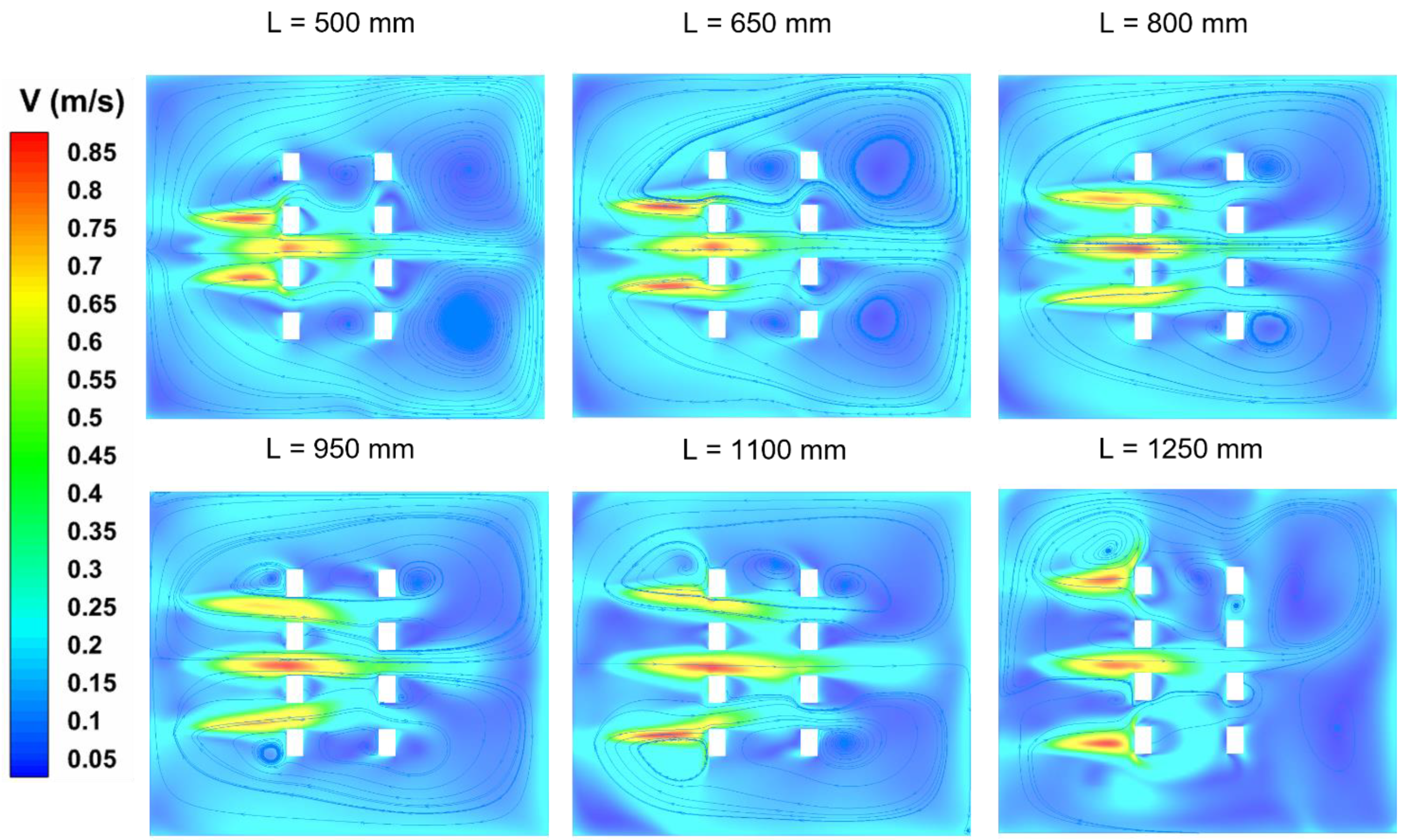
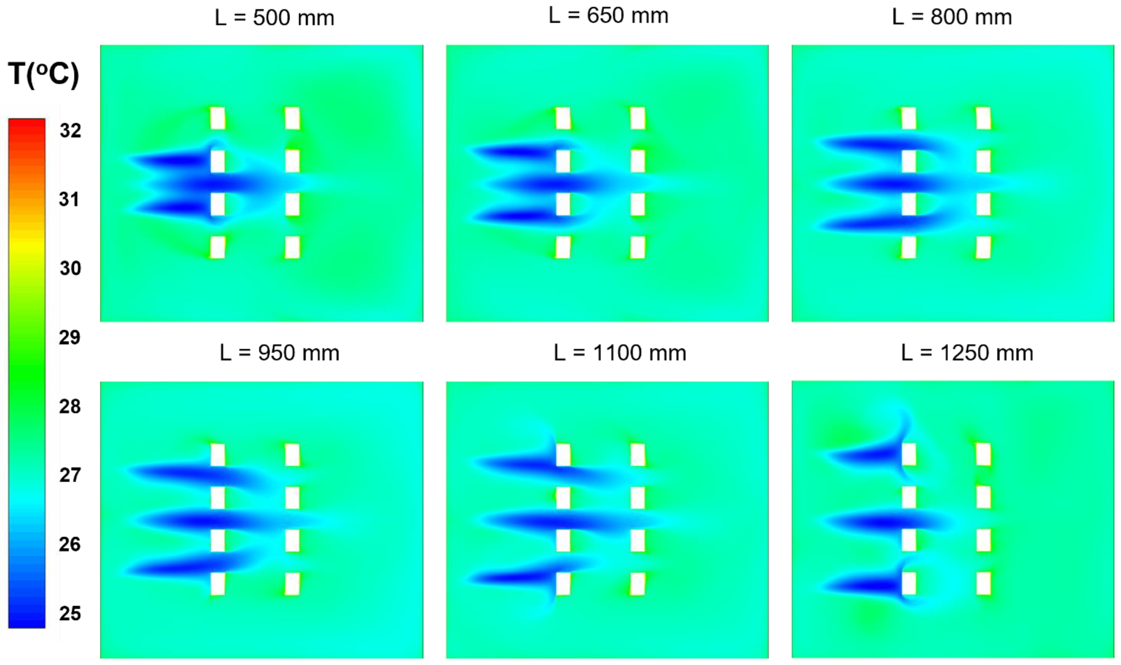
3.3.1. Airflow Characteristics

When multiple small jets from several adjacent air inlets flowed along the jet direction and reached a specific distance, the small jets merged into one large jet. The distance between the merge point of the jets and the air inlet was determined by the spacing between the adjacent air inlets. Air inlets with small spacing were prone to cause a negative pressure zone in the central area, which accelerated the merging of the edge jet to the central jet. The interaction between the air jets directly affected the indoor environment; thus, three typical air inlet spacings from the numerical simulation results were selected for comprehensive analysis.

Figure 10 shows the sectional velocity distribution contours for x = 1.5 m, 1.7 m, and 1.9 m with supply air inlet spacings of 500 mm, 950 mm, and 1100 mm, respectively. Three parallel jets at L = 500 mm began to overlap, affecting the air distribution in the occupied zone at x = 1.5 m. The velocity distribution contour clearly shows the peak velocity in the overlapping area; the velocity of the three parallel jets tends to decrease with an increase in the distance between the jet body and the air inlet. However, there was no obvious overlap between the 950 mm and 1100 mm spacings. The supply air formed three independent air jets as the distance increased and started to overlap in the lower half of the axial plane instead of forming a confluence in the horizontal planes of the air inlets. Previous studies [34,53] have shown that the velocity profile exhibits a strong asymmetry of its center downstream of the horizontal non-isothermal jet, mainly caused by the strong mixing of the lower part of the jet. The upper part formed a stable temperature and velocity layer; the lower part did not. Thus, the merging of the lower part of multiple parallel non-isothermal jets became stronger with an increase in the distance between the jet body and the air inlet.

Figure 11 and Figure 12 show the velocity distribution contour and temperature distribution contour in the plane z = 1.1 m at different air inlet spacings, respectively. Most of the main bodies of the jet with a 500 mm supply air inlet spacing overlapped each other to form a concentrated jet coverage area with a high air velocity. However, there was an obvious area with inadequate airflow on both sides of the occupied zone, where occupants may feel too warm. In addition, there were two large eddy regions on both sides of the rear of the room. The overlapping area of the jet gradually decreased with increasing supply air inlet spacing, which also increased the horizontal coverage area. The airflow on both sides of the occupied zone became stronger, and the air velocity in front of the second row of personnel was more uniform. In addition, the eddy regions at the rear of the room were also improved. When the supply air inlet spacing was increased to 950 mm, the overlapping area of the three jets in front of the first row of personnel also gradually decreased, and an area that could not be completely covered appeared between the jets. Insufficient airflow directly affects the thermal environment of an area. As the air inlet spacing increased to 1250 mm, the three jets were almost sent into the occupied zone in isolation with no confluence. The airflow in some areas between the jets was insufficient, and some areas between jets were almost unaffected by the jets. Additionally, the air inlets on both sides faced the first row of occupants. Although the jets were isolated before reaching the first row of occupants, the range of the jets widened owing to the blocking effect of the occupants. The thermal environment of the area that could not be fully covered between the jets can also be improved. Moreover, the eddy flows appeared on both sides of the room near the air inlets. Through comprehensive analysis of the change process of indoor air distribution with different supply air inlet spacings, it was found that there was a more appropriate range of supply air inlet spacing in which a more comfortable thermal environment could be produced in the occupied zone.

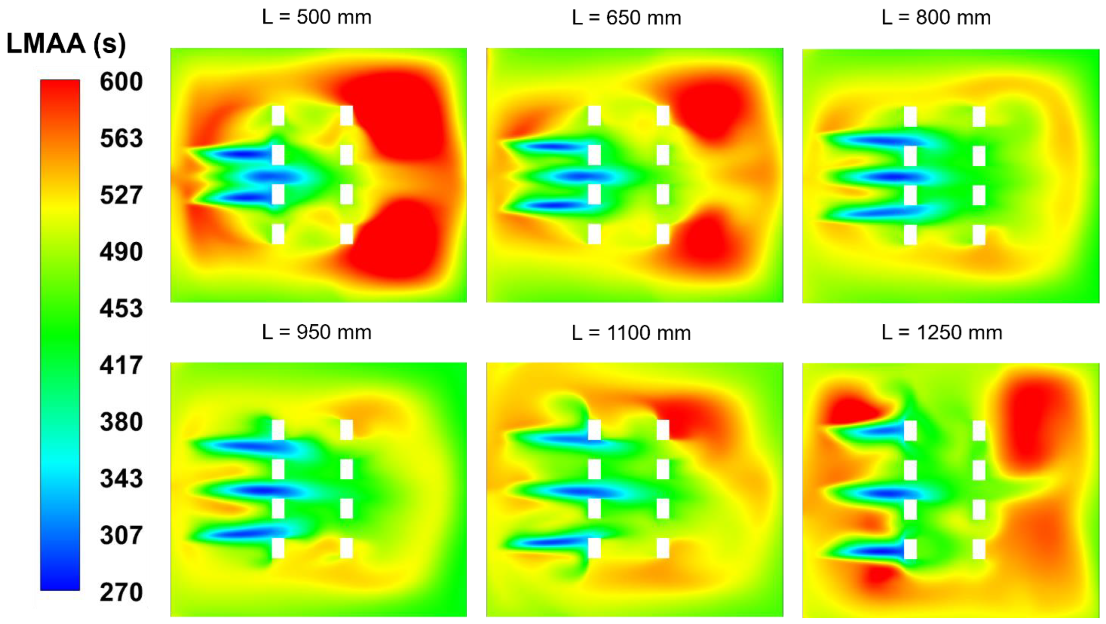
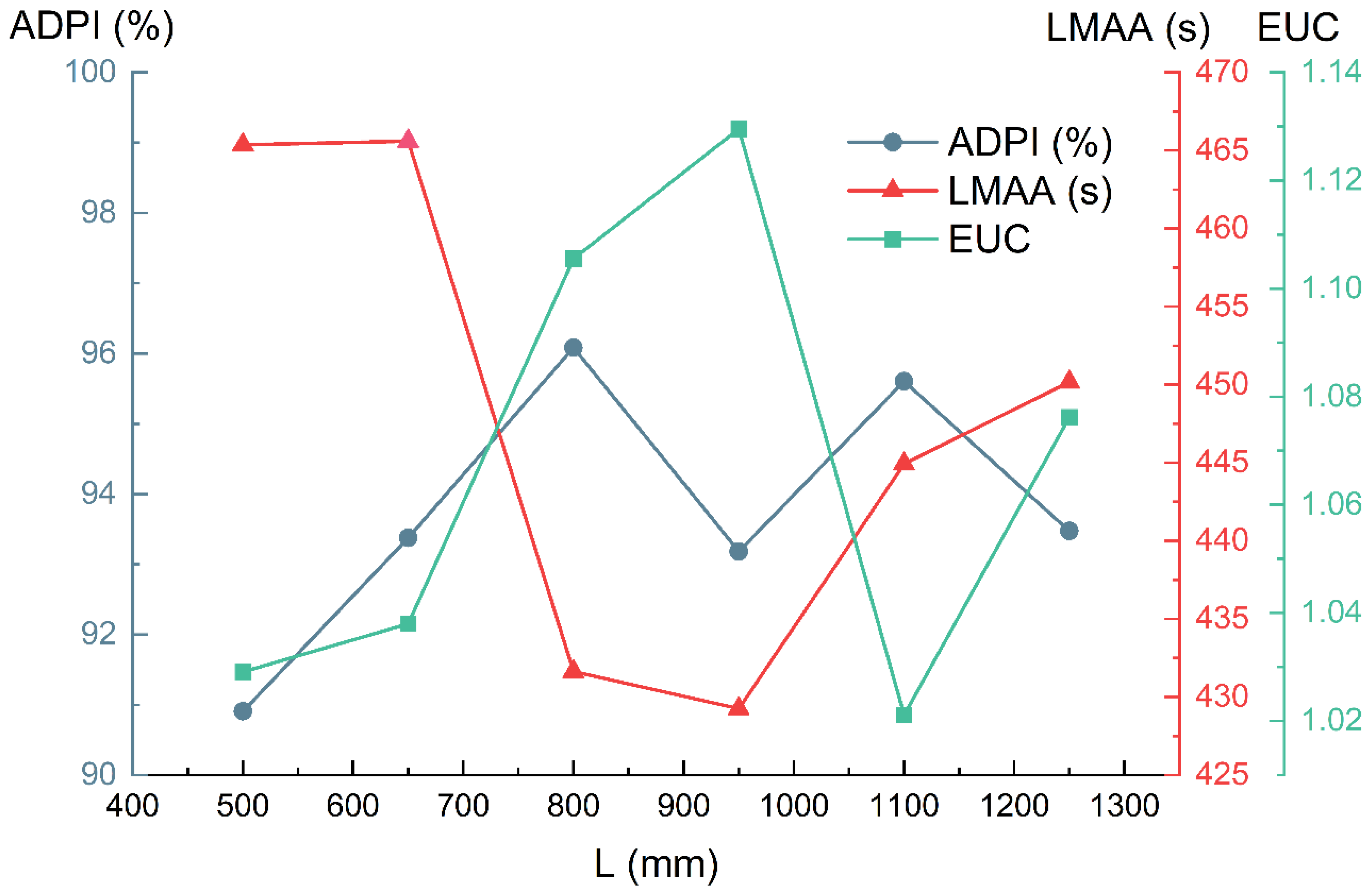
3.3.2. Analysis of Evaluation Indices

Figure 13 presents the ADPI distribution in the EDTS velocity diagram at different air inlet spacings. In the occupied zone, approximately 1500 nodes were used for the calculations of the ADPI. The ADPI values were all above 90% at different supply air inlet spacings, indicating that SV could be in full compliance with the stipulation of the ADPI in ASHRAE 113-2013 [54]. The results also indicated the good thermal comfort performance of SV. Most of the nodes were concentrated in the upper left corner of the square frame, indicating that the room with SV effectively improved the thermal neutral temperature at a low air velocity. When the supply air inlet spacing was greater than 500 mm, the ADPI value did not increase significantly, indicating that when the spacing was greater than a certain value, the ADPI value was only slightly affected.

Figure 14 shows that the lowest mean air age occurred when the air inlet spacing was 800–1100 mm, indicating that better air distribution and air quality in the occupied zone were created when the spacing was within this range. A jet with a smaller air inlet spacing was more concentrated with a higher air velocity, which lowered the local age of the air. However, the local mean age of air in the area on the sides of the room was significantly greater than in other areas owing to insufficient air movement, resulting in a greater mean age of air in the entire occupied zone. The jets from large supply air inlet spacings were isolated from each other, forming an area between the jets that could not be covered, leading to a weak airflow and greater age of air. Although the index was lower in the area through which the isolated jet passed, the mean age of air in the entire room was also greater.

Figure 15 shows the variation in the index values with different air inlet spacings. As the supply air spacing increased from 500 mm, the ADPI value started to increase gradually, reaching a maximum when the spacing reached 800 mm before fluctuating. The change trend of the EUC was similar; however, the maximum value occurred when the spacing was 950 mm. The LMAA value changed little when the spacing increased to 650 mm and then decreased sharply to 430 s at a spacing of 950 mm. When the spacing exceeded 950 mm, the LMAA rebounded to 450 s as the spacing increased. The optimal values of ADPI, ECU, and LMAA correspond to air inlet spacings of 800 mm, 950 mm, and 950 mm, respectively. Thus, it was impossible to specify the optimum inlet spacing directly. A comprehensive optimal supply air inlet spacing can be obtained through multi-objective optimization analysis.

3.4. Optimization of Air Inlet Spacing

The Technique for Order of Preference by Similarity to Ideal Solution (TOPSIS) is a method of ranking according to the proximity between a limited number of evaluation objects and the idealized target. It is also a common and effective method for multi-objective decision analyses [55,56]. The TOPSIS method determines the optimal object with the shortest distance to a positive ideal solution and the longest distance to a negative ideal solution [57]. Thus, it was used to calculate the optimal spacing of the air inlets with SV, as shown in Figure 16. The details on the procedure for TOPSIS were enclosed in Supplementary Materials.

The final calculations are presented in

Table 7. Calculation results of TOPSIS evaluation method.

Spacing of Air Inlet	Relative Fit Degree	Ranking
500	0.0476	6
650	0.1001	5
800	0.8560	1
950	0.9010	2
1100	0.4019	4
1250	0.5283	3

. The weight factors for ADPI, LMAA, and EUC were 0.21, 0.40, and 0.39, respectively. The best performance was achieved with an air inlet spacing of 800 mm, and the worst performance was achieved with an air inlet spacing of 500 mm. Based on the calculation results, compared with a spacing of 500 mm, a spacing of 800 mm increased ADPI by 5.7%, decreased mean age of air by 7.2%, and increased EUC by 7.4%.

4. Conclusions

This paper presents an optimization study of the supply air inlet spacing in a room with SV. Experiments and numerical simulations were performed to study the influence of air inlet spacing on the air distribution in the occupied zone. The air velocity and temperature distributions were analyzed with different air inlet spacings. Evaluation indices (ADPI, LMAA, and EUC) were used to evaluate the effect of air inlet spacing on the ventilation performance of the SV. In addition, six axial velocity attenuation formulas for the jet were verified using experimental data. After a comprehensive analysis of the evaluation index results, the optimal air inlet spacing was studied using the multi-objective optimization method TOPSIS, and the optimal spacing under the simulated condition was obtained. The main conclusions are summarized as follows.

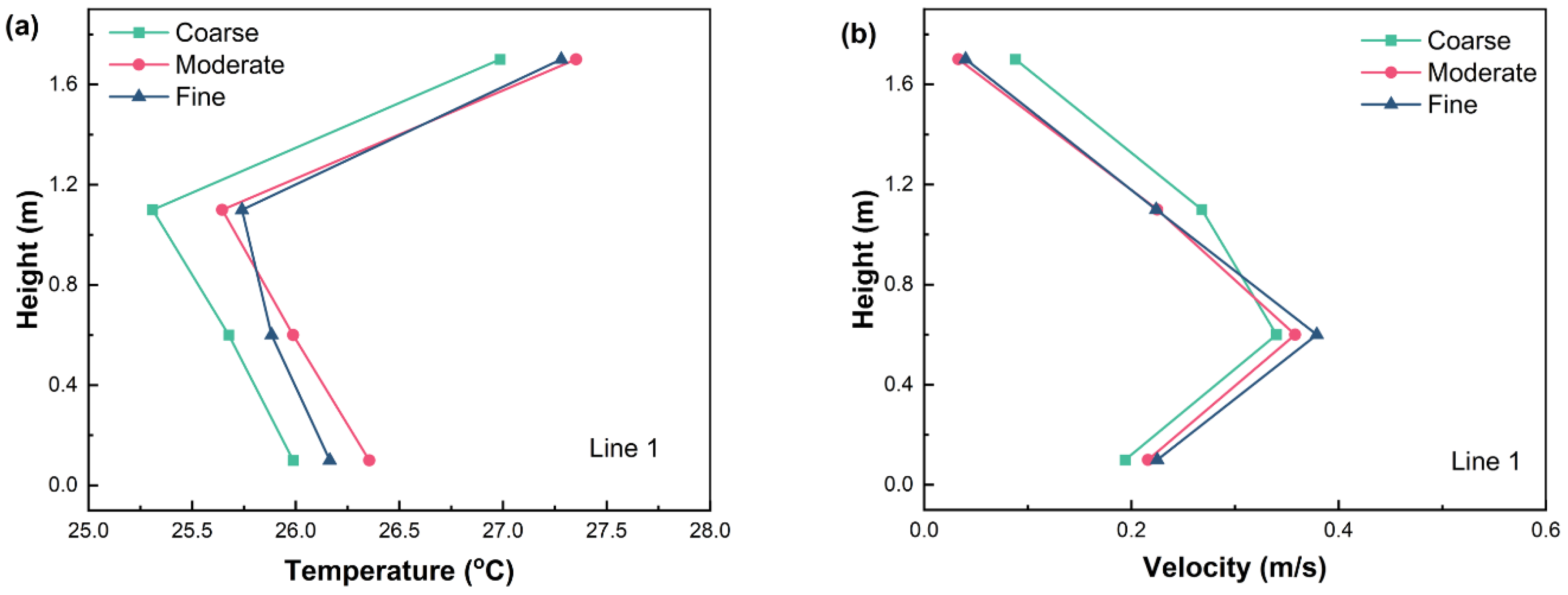
• Analysis of the experimental results showed that the flow characteristics in the occupied zone of the room were significantly different with different spacings of the supply air inlets, and the thermal comfort may be different at the same location. The position close to the air inlet was directly affected by the air inlet spacing. For locations away from the air inlets, the change in air temperature with spacing was more obvious than that of air velocity owing to the blocking effect of personnel.
• The attenuation formula for the jet axial velocity was verified using the measured data. The RMSE between the measured data and the predicted values for the three cases were 0.23 m/s, 0.09 m/s, and 0.18 m/s, respectively. Thus, the modified Abramovich formula is the most suitable for attenuation of the axial velocity of multiple parallel jets in SV rooms.
• Numerical simulation results showed that inappropriate air inlet spacing was not conducive to the performance of indoor air distribution. The distance between the merge point of the parallel jet and the air inlet depended on the spacing between the adjacent air inlets. A small air inlet spacing led to a concentration of the conditioned supply air in the middle of the room, and the indoor thermal environment on both sides could not be guaranteed. A large spacing resulted in areas that could not be covered by the supply air. The velocity profile showed strong asymmetry in its center downstream of the horizontal non-isothermal jet, mainly caused by the strong mixing of the lower part of the jet.
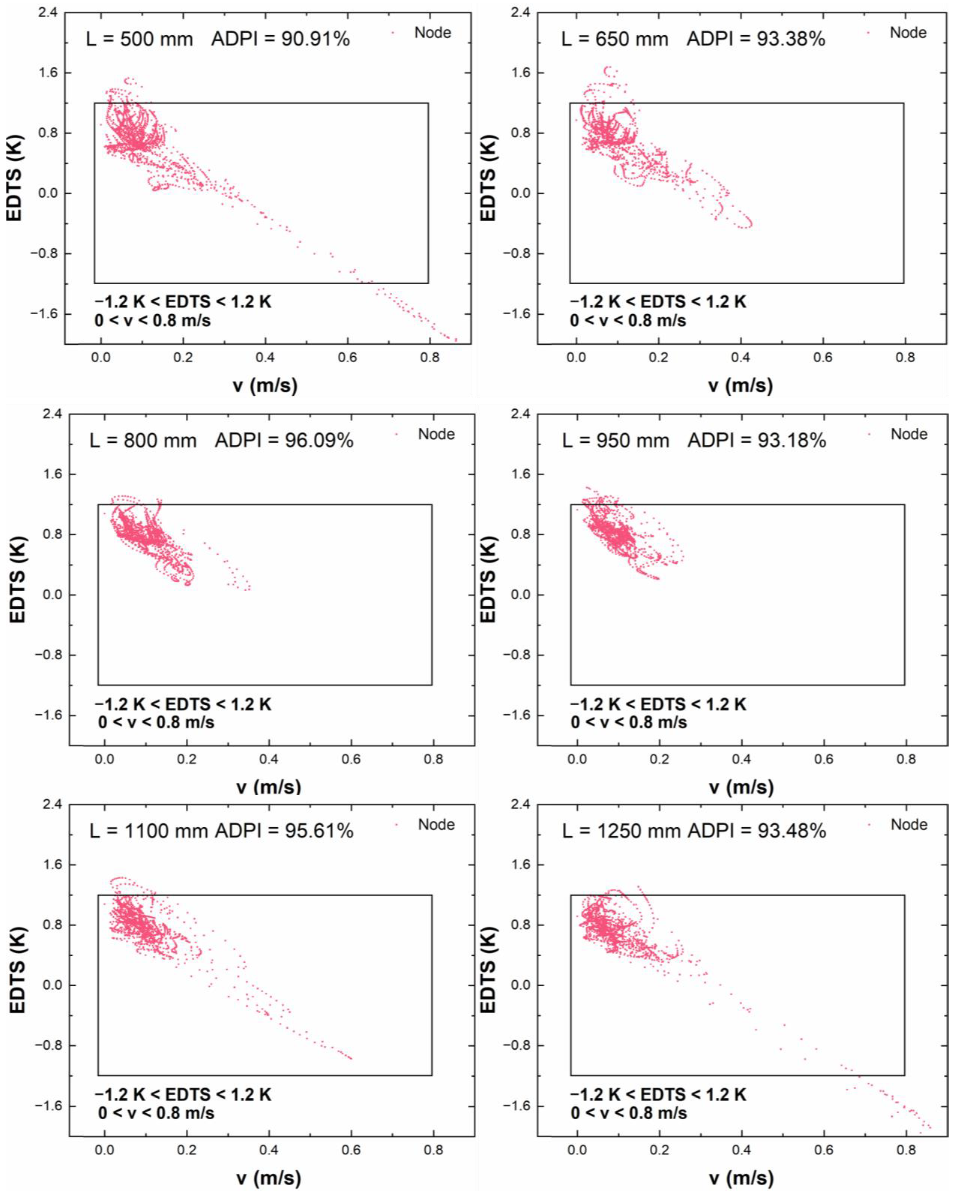
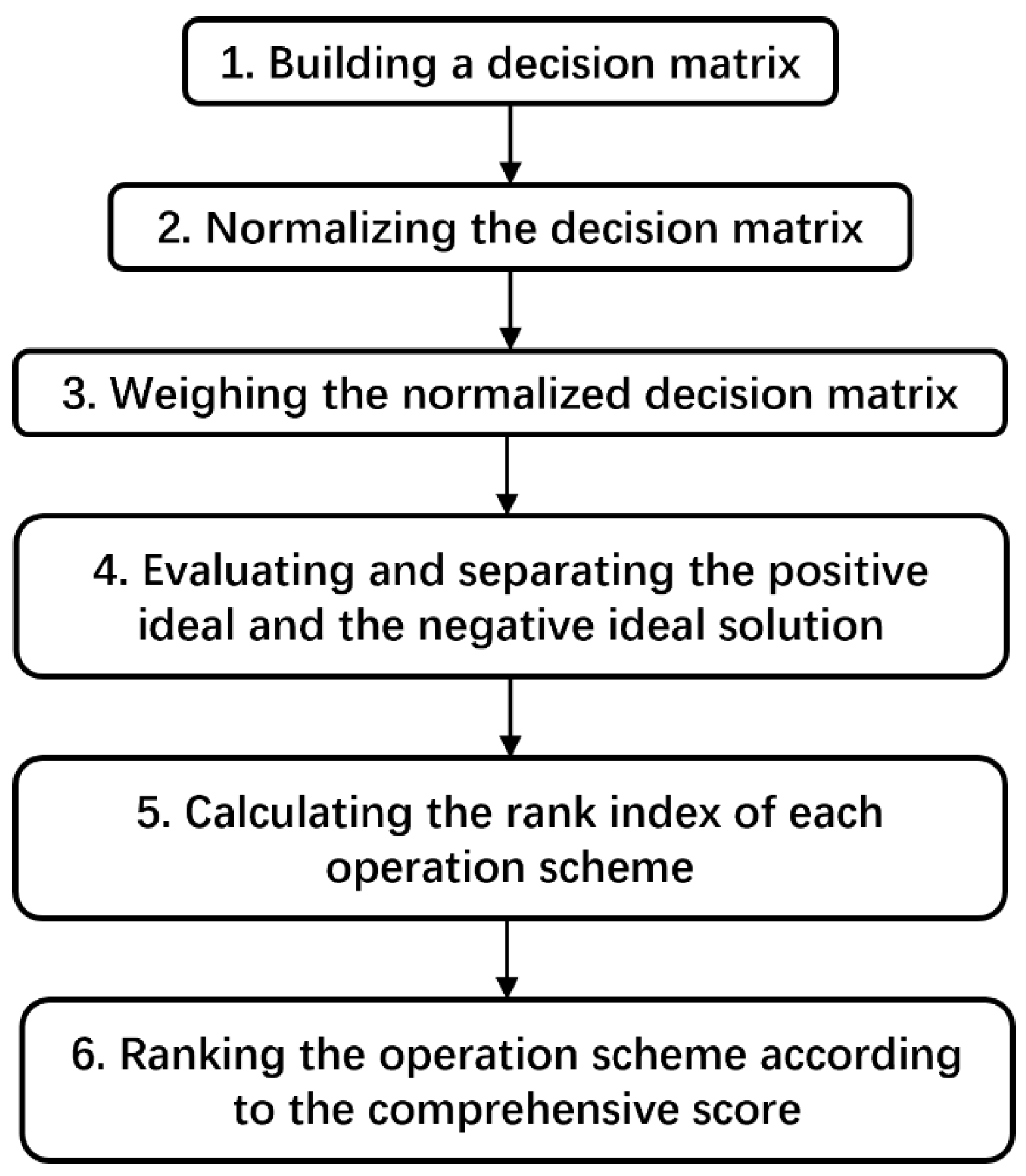
• By analyzing the influence of air inlet spacing on the three evaluation indices, it was found that the optimal value of ADPI corresponded to an air inlet spacing of 800 mm; the optimal LMAA and EUC corresponded to an air inlet spacing of 950 mm. The multi-objective optimization method TOPSIS was used to optimize the air inlet spacing. The optimal spacing was 800 mm.

References

1. Orosa, J.A.; Kameni Nematchoua, M.; Reiter, S. Air Changes for Healthy Indoor Ambiences under Pandemic Conditions and Its Energetic Implications: A Galician Case Study. Appl. Sci. 2020, 10, 7169. [Google Scholar] [CrossRef]
2. Krzaczek, M.; Florczuk, J.; Tejchman, J. Improved energy management technique in pipe-embedded wall heating/cooling system in residential buildings. Appl. Energy 2019, 254, 113711. [Google Scholar] [CrossRef]
3. Jung, W.; Jazizadeh, F. Human-in-the-loop HVAC operations: A quantitative review on occupancy, comfort, and energy-efficiency dimensions. Appl. Energy 2019, 239, 1471–1508. [Google Scholar] [CrossRef]
4. Yang, B.; Melikov, A.K.; Kabanshi, A.; Zhang, C.; Bauman, F.S.; Cao, G.; Awbi, H.; Wigö, H.; Niu, J.; Cheong, K.W.D.; et al. A review of advanced air distribution methods-theory, practice, limitations and solutions. Energy Build. 2019, 202, 109359. [Google Scholar] [CrossRef] [Green Version]
5. Nie, X.; Chen, Z.; Zhu, Z. Assessment of Low-Reynolds Number k-&epsilon; Models in Prediction of a Transitional Flow with Coanda Effect. Appl. Sci. 2023, 13, 1783. [Google Scholar]
6. Segala, G.; Doriguzzi-Corin, R.; Peroni, C.; Gazzini, T.; Siracusa, D. A Practical and Adaptive Approach to Predicting Indoor CO2. Appl. Sci. 2021, 11, 10771. [Google Scholar] [CrossRef]
7. Park, S.; Park, H.; Seo, J. Analysis on the Exhaust Air Recirculation of the Ventilation System in Multi-Story Building. Appl. Sci. 2021, 11, 4441. [Google Scholar] [CrossRef]
8. Zhang, S.; Niu, D.; Lin, Z. Occupancy-aided ventilation for airborne infection risk control: Continuously or intermittently reduced occupancies? Build. Simul. 2022. [Google Scholar] [CrossRef]
9. Zhang, S.; Lu, Y.L.; Niu, D.; Lin, Z. Energy performance index of air distribution: Thermal utilization effectiveness. Appl. Energy 2022, 307, 118122. [Google Scholar] [CrossRef]
10. Olstrup, H.; Hagenbjork, A.; Orru, H. Ventilation Systems and Their Impact on Nanoparticle Concentrations in Office Buildings. Appl. Sci. Basel 2021, 11, 8930. [Google Scholar] [CrossRef]
11. Danca, P.; Coşoiu, C.I.; Nastase, I.; Bode, F.; Georgescu, M.R. Personalized Ventilation as a Possible Strategy for Reducing Airborne Infectious Disease Transmission on Commercial Aircraft. Appl. Sci. 2022, 12, 2088. [Google Scholar] [CrossRef]
12. Lin, Z.; Chow, T.T.; Tsang, C.F. Stratum ventilation-A conceptual introduction. In Proceedings of the 10th International Conference on Indoor Air Quality and Climate, Beijing, China, 4–9 September 2005; Volume 1–5, pp. 3260–3264. [Google Scholar]
13. Lin, Z.; Yao, T.; Chow, T.T.; Fong, K.F.; Chan, L.S. Performance evaluation and design guidelines for stratum ventilation. Build. Environ. 2011, 46, 2267–2279. [Google Scholar] [CrossRef]
14. Lin, Z.; Chow, T.T.; Tsang, C.F.; Fong, K.F.; Chan, L.S. Stratum ventilation—A potential solution to elevated indoor temperatures. Build. Environ. 2009, 44, 2256–2269. [Google Scholar] [CrossRef]
15. Fong, M.L.; Lin, Z.; Fong, K.F.; Chow, T.T.; Yao, T. Evaluation of thermal comfort conditions in a classroom with three ventilation methods. Indoor Air 2011, 21, 231–239. [Google Scholar] [CrossRef] [PubMed]
16. Lin, Z.; Lee, C.K.; Fong, S.; Chow, T.T.; Yao, T.; Chan, A.L.S. Comparison of annual energy performances with different ventilation methods for cooling. Energy Build. 2011, 43, 130–136. [Google Scholar] [CrossRef]
17. Cheng, Y.; Lin, Z.; Fong, A.M.L. Effects of temperature and supply airflow rate on thermal comfort in a stratum-ventilated room. Build. Environ. 2015, 92, 269–277. [Google Scholar] [CrossRef]
18. Lin, Z. Stratum ventilation-a low-carbon way to thermal comfort and indoor air quality. Int. J. Low Carbon Technol. 2017, 12, 323–329. [Google Scholar] [CrossRef] [Green Version]
19. Tian, L.; Lin, Z.; Wang, Q. Comparison of gaseous contaminant diffusion under stratum ventilation and under displacement ventilation. Build. Environ. 2010, 45, 2035–2046. [Google Scholar] [CrossRef]
20. Zhang, S.; Cheng, Y.; Oladoku, M.O.; Lin, Z. Subzone control method of stratum ventilation for thermal comfort improvement. Build. Environ. 2019, 149, 39–47. [Google Scholar] [CrossRef] [Green Version]
21. Zhang, S.; Cheng, Y.; Lin, Z. Robust evaluation method of thermal deviation of air distribution. Build. Environ. 2019, 158, 217–225. [Google Scholar] [CrossRef]
22. Cheng, Y.; Lin, Z. Technical feasibility of a stratum-ventilated room for multiple rows of occupants. Build. Environ. 2015, 94, 580–592. [Google Scholar] [CrossRef]
23. Wu, W.Q.; Lin, Z. An experimental study of the influence of a walking occupant on three air distribution methods. Build. Environ. 2015, 85, 211–219. [Google Scholar] [CrossRef]
24. Yao, T.; Lin, Z. An experimental and numerical study on the effect of air terminal layout on the performance of stratum ventilation. Build. Environ. 2014, 82, 75–86. [Google Scholar] [CrossRef]
25. Fong, M.L.; Hanby, V.; Greenough, R.; Lin, Z.; Cheng, Y. Acceptance of thermal conditions and energy use of three ventilation strategies with six exhaust configurations for the classroom. Build. Environ. 2015, 94, 606–619. [Google Scholar] [CrossRef]
26. Zheng, X.; Jian, X.; Wei, J.; Wenzheng, D. Numerical and Experimental Investigation of Near-Field Mixing in Parallel Dual Round Jets. Int. J. Aerosp. Eng. 2016, 2016, 7935101. [Google Scholar] [CrossRef] [Green Version]
27. Yin, Z.; Zhang, H.; Lin, J. Experimental Study on the Flow Field Characteristics in the Mixing Region of Twin Jets. J. Hydrodyn. 2007, 19, 309–313. [Google Scholar] [CrossRef]
28. Liu, Z.; Xu, T.; Shi, E. Study of the aerodynamical characteristics of mutiple parallel jets. J. Xian Jiaotong Univ. 1989, 4, 73–81. [Google Scholar]
29. Wang, X.K.; Tan, S.K. Experimental investigation of the interaction between a plane wall jet and a parallel offset jet. Exp. Fluids 2007, 42, 551–562. [Google Scholar] [CrossRef]
30. Mondal, T.; Das, M.K.; Guha, A. Periodic vortex shedding phenomenon for various separation distances between two plane turbulent parallel jets. Int. J. Heat Mass Transf. 2016, 99, 576–588. [Google Scholar] [CrossRef]
31. Liu, P.Y.; Zhang, H.; Wu, Y.X.; Zhang, M.; Lu, J.F. Experimental study on the flow interaction of two parallel rectangular jets through exits with sudden contraction. Exp. Therm. Fluid Sci. 2017, 88, 622–631. [Google Scholar] [CrossRef]
32. Cheng, Y.; Zhang, S.; Huan, C.; Oladokun, M.O.; Lin, Z. Optimization on fresh outdoor air ratio of air conditioning system with stratum ventilation for both targeted indoor air quality and maximal energy saving. Build. Environ. 2019, 147, 11–22. [Google Scholar] [CrossRef] [Green Version]
33. Cheng, F.H.; Zhang, S.; Gao, S.S.; Tian, X.; Liao, C.H.; Cheng, Y. Experimental investigation of airflow pattern and turbulence characteristics of stratum ventilation in heating mode. Build. Environ. 2020, 186, 107339. [Google Scholar] [CrossRef]
34. Xu, D.; Chen, J. Experimental study of stratified jet by simultaneous measurements of velocity and density fields. Exp. Fluids 2012, 53, 145–162. [Google Scholar] [CrossRef]
35. Xiao, Y.; Liu, X.; Yang, Y. Study on Jet Coincidence Characteristics of Air Supply Outlet in Large Space. Build. Energy Environ. 1997, 3, 1–5. [Google Scholar]
36. Zhou, Y.; Wang, S.; Peng, R.; Hua, C. Study on the calculation method of air distribution in stratified air conditioning. J. HVAC 1983, 2, 1–6+19. [Google Scholar]
37. Zhao, J. Theoretical and Experimental Study on the Coincidence Characteristics of Multi-Stream Air Supply Jet in Large Space; Tongji University: Shanghai, China, 2000. [Google Scholar]
38. ASHRAE. ASHRAE Handbook Fundamentals; ASHRAE Inc.: Atlanta, GA, USA, 2005. [Google Scholar]
39. Li, A. Unity of air jet buoyant plume and buoyant jet. J. HVAC 1998, 28, 8–10. [Google Scholar]
40. Chen, Q.Y. Ventilation performance prediction for buildings: A method overview and recent applications. Build. Environ. 2009, 44, 848–858. [Google Scholar] [CrossRef]
41. Mao, N.; Song, M.J.; Chan, M.Y.; Pan, D.M.; Deng, S.M. Computational fluid dynamics (CFD) modelling of air flow field, mean age of air and CO2 distributions inside a bedroom with different heights of conditioned air supply outlet. Appl. Energy 2016, 164, 906–915. [Google Scholar] [CrossRef]
42. Zhang, Z.; Zhai, Z.Q.; Zhang, W.; Chen, Q.Y. Evaluation of various turbulence models in predicting airflow and turbulence in enclosed environments by CFD: Part 2-comparison with experimental data from literature. HvacR Res. 2007, 13, 871–886. [Google Scholar] [CrossRef]
43. ANSYS Inc. ANSYS Fluent Theory Guide; ANSYS Inc.: Canonsburg, PA, USA, 2013. [Google Scholar]
44. Heiselberg, P. Draught risk from cold vertical surfaces. Build. Environ. 1994, 29, 297–301. [Google Scholar] [CrossRef] [Green Version]
45. Awbi, H.B. Calculation of convective heat transfer coefficients of room surfaces for natural convection. Energy Build. 1998, 28, 219–227. [Google Scholar] [CrossRef]
46. Pereira, P.F.d.C.; Broday, E.E.; Xavier, A.A.d.P. Thermal Comfort Applied in Hospital Environments: A Literature Review. Appl. Sci. 2020, 10, 7030. [Google Scholar] [CrossRef]
47. Lin, Z. Effective draft temperature for evaluating the performance of stratum ventilation. Build. Environ. 2011, 46, 1843–1850. [Google Scholar] [CrossRef]
48. Liu, J.; Lin, Z. Energy and Exergy Performances of Floor, Ceiling, Wall Radiator and Stratum Ventilation Heating Systems for Residential Buildings. Energy Build. 2020, 220, 110046. [Google Scholar] [CrossRef]
49. Tian, L.; Lin, Z.; Liu, J.; Yao, T.; Wang, Q.W. The impact of temperature on mean local air age and thermal comfort in a stratum ventilated office. Build. Environ. 2011, 46, 501–510. [Google Scholar] [CrossRef]
50. Buratti, C.; Palladino, D. Mean Age of Air in Natural Ventilated Buildings: Experimental Evaluation and CO2 Prediction by Artificial Neural Networks. Appl. Sci. 2020, 10, 1730. [Google Scholar] [CrossRef] [Green Version]
51. Chen, F.J.; Chen, H.X.; Xie, J.L.; Shu, Z.H.; Mao, J.N. Air distribution in room ventilated by fabric air dispersion system. Build. Environ. 2011, 46, 2121–2129. [Google Scholar] [CrossRef]
52. Cheng, Y.; Lin, Z.; Yao, T.; Wu, W. Numerical comparison of indoor air quality and local thermal comfort in a classroom with three ventilation methods. In Proceedings of the 13th International Conference on Indoor Air Quality and Climate, Indoor Air 2014, Hong Kong, China, 7–12 July 2014; pp. 68–75. [Google Scholar]
53. Ghaisas, N.S.; Shetty, D.A.; Frankel, S.H. Large eddy simulation of turbulent horizontal buoyant jets. J. Turbul. 2015, 16, 772–808. [Google Scholar] [CrossRef]
54. ANSI/ASHRAE Standard 113-2013; Method of Testing for Room Air Diffusion. ANSI: Washington, DC, USA, 2013.
55. Behzadian, M.; Khanmohammadi Otaghsara, S.; Yazdani, M.; Ignatius, J. A state-of the-art survey of TOPSIS applications. Expert Syst. Appl. 2012, 39, 13051–13069. [Google Scholar] [CrossRef]
56. Fan, Y. A TOPSIS optimization for the indoor thermal environment through oscillating airflow generated from a cassette split type air conditioner. Indoor Built Environ. 2021, 30, 1200–1210. [Google Scholar] [CrossRef]
57. Mao, N.; Song, M.; Deng, S. Application of TOPSIS method in evaluating the effects of supply vane angle of a task/ambient air conditioning system on energy utilization and thermal comfort. Appl. Energy 2016, 180, 536–545. [Google Scholar] [CrossRef]
Figure 1. Experimental platform: (a) laboratory layout; (b) layout plan of sampling lines.
Applsci 13 04143 g001
Figure 2. Layout plan of measurement points in center plane of multiple parallel jets.
Applsci 13 04143 g002
Figure 3. Multiple parallel jets.
Applsci 13 04143 g003
Figure 4. Computational model (unit: mm).
Applsci 13 04143 g004
Figure 5. Mesh of computational domain: (a) 3D mesh; (b) Z = 1.1m.
Applsci 13 04143 g005aApplsci 13 04143 g005b
Figure 6. Comparison of different grid numbers: (a) air temperature; (b) air velocity.
Applsci 13 04143 g006
Figure 7. Comparison of different turbulence models and experiments: (a) air temperature of Line 1; (b) air temperature of Line 4; (c) air velocity of Line 1; (d) air velocity of Line 4.
Applsci 13 04143 g007
Figure 8. Comparison of theoretical models and actual measurements of axial velocity attenuation of the main part of multiple parallel jets: (a) L = 650 mm, V0 = 2.02 m/s; (b) L = 650 mm, V0 = 1.53 m/s; (c) L = 1300 mm, V0 = 2.02 m/s.
Applsci 13 04143 g008
Figure 9. Lines 1–4 of four experimental cases at 1.1 m above floor: (a) air temperature; (b) air velocity.
Applsci 13 04143 g009
Figure 10. Velocity distribution contour for x = 1.5 m, 1.7 m, and 1.9 m for three air inlet spacings.
Applsci 13 04143 g010
Figure 11. Velocity distribution contour in the plane z =1.1 m with different air inlet spacings.
Applsci 13 04143 g011
Figure 12. Temperature distribution contour in the plane z = 1.1 m with different air inlet spacings.
Applsci 13 04143 g012
Figure 13. ADPI distribution in EDTS–velocity diagram with different air inlet spacings.
Applsci 13 04143 g013
Figure 14. Contour of local mean air age in the plane z = 1.1 m with different air inlet spacings.
Applsci 13 04143 g014
Figure 15. Diagram of ADPI, LMAA, and EUC in the plane z = 1.1 m with different air inlet spacings.
Applsci 13 04143 g015
Figure 16. Flow chart of TOPSIS optimization method.
Applsci 13 04143 g016