Damage Creep Model of Viscoelastic Rock Based on the Distributed Order Calculus

Abstract

In this paper, the distributed order calculus was used to establish a creep damage theoretical model to accurately describe the creep properties of viscoelastic materials. Firstly, the definition and basic properties in math of the distributed order calculus were given. On this basis, the mechanical elements of the distributed order damper were built to describe the viscoelastic properties. Then, the distributed order damper was introduced into the three-parameter solid model to establish the distributed order three-parameter solid model. The inverse Laplace transform derived the operator’s contour integrals and the path integrals along Hankel’s path. The integral properties were analysed. Next, the creep properties and relaxation characteristics of the distributed order three-parameter solid model were studied in detail. Finally, taking the rock materials as an example, the distributed order damage damper model was established. Its operator integrals were calculated, and the properties were discussed. Meanwhile, taking the integer-order Nishihara model as the standard, the distributed order damage creep combined model of the rock mass was constructed. The calculation examples were given to study the damage creep properties of the rock mass.

1. Introduction

Viscous-elastic materials have been widely applied in industrial development and infrastructure development, such as plastics, rubbers, pitches, epoxy resins, etc. Because of mechanical behaviours, they show both elastic solid and viscous fluid behaviours under external loads [1]. The former behaviour can ensure the strength and stiffness of materials, and the latter can endow materials with large-deformation capacity and better environmental adaptability [2,3].

Viscoelastic materials are widely applied in the field of artificial synthetic materials. Many geologic materials in nature belong to typical viscoelastic materials, such as rocks [4]. Under normal states of average temperature, dryness, and no confining pressure, rocks have typical brittle characteristics, that is, single elastic solid mechanical behaviours [5]. In addition, they also show remarkable viscous fluid behaviours under specific environments. During underground coal mining, rocks exhibit brittleness behaviours with small deformation under an external low-stress state, while they present obvious continuous prominent deformation behaviours and viscous fluid behaviours under deep high confining pressure [6]. Moreover, they also show significant viscoelastic characteristics under high temperatures and in water-rich environments [7].

Viscoelastic materials will continuously increase deformation under external loads, called creep deformation [8]. The continuous creep deformation will damage the materials and make the structure unstable [9]. The basic premise of establishing an accurate creep damage model is to reveal the instability mechanisms of the structure of viscoelastic materials based on experimental mechanical results [10]. Scholars have constructed several creep models of viscoelastic materials based on mathematical and mechanical theories, which can provide theoretical references for the analysis of materials’ viscoelastic and creep damage characteristics. The basic models established by the classical theory of mechanics, such as the Maxwell model, Kelvin model, three-parameter solid models, etc., can reflect rock materials’ deformation characteristics in the stages of instantaneous elasticity, constant creep, and accelerated creep [11]. Based on these basic models, some complex models have been established to describe the whole creep process of rocks, including the Poyting-Thomson model and visco-elastoplastic models, etc. [12,13,14,15]. The creep above models can reflect the deformation characteristics of rock creep in various stages. They essentially reflect the stress and deformation characteristics of rocks at certain points. However, the creep failure of rocks is caused by damage accumulation at different times [16]. Therefore, classical theories have limitations. Compared to classical theories, fractional calculus theory focuses on the research of the creep deformation of rocks and can accurately describe global characteristics [17,18].

Fractional calculus can better describe behaviours with time memory, which can overcome the limitations of the definition of local limits of time derivatives in integral calculus [19,20,21]. It can accurately describe the path dependence of abnormal mechanical behaviours in the complex fractal structure [22]. In theory, the fractional Laplace operator is known as a typical non-local fractional derivative, which makes the fractional calculus span the classical theory of mechanics established based on Euclidean geometry and the absolute space-time point. Fractional calculus has been widely used to describe the viscoelastic characteristics of materials [23,24].

Distributed order derivatives are developed from single fractional derivative models. M. Caputo originally proposed the concept in 1969 [25]. It involves the use of a series of fractional derivatives with different weights to replace the single fractional derivative. The distributed order operator is defined by the analytic expression by integrating parts of a power series for a long time, and the application effects are poor. There are two types of application conditions for the distributed order equations. One involves the use of fractional order theory to simulate the essence of physical conditions, and the other involves confining the fractional order to a specific area continuously. Compared with the fractional order model, the distributed order model could describe the same complex problem with a more straightforward structure and could ensure accuracy simultaneously.

After nearly 50 years, the distributed order theory and its practical applications have obtained great achievements. Caputo and Bagley et al. proposed the electrolyte diffusion distributed order equations and the distributed order filter [26]. Lorenzo et al. analysed and discussed various operators’ definitions and physical meanings, transformation forms, and memory characteristics in kernel functions [23]. Atanackovic et al. discussed the properties of solutions for equations of distributed order viscoelastic rods and analysed the properties of kernel functions in detail [27]. Bagley and Torvik studied solutions to Cauchy problems in diffusion equations by the distributed order theory [28]. In recent years, the distributed order calculus theory has made significant progress, including the theoretical research of distributed order equations [29,30,31], unique functions in distributed order theories [32,33,34], and numerical methods of distributed order equations [35,36,37]. Some scholars also applied the distributed order theories to study the physical characteristics of systems, such as non-linear complexity [38,39,40], network structure [41], non-homogeneous phenomena [42,43], and multiscale and multi-space phenomena, etc. [33,44]. The research on the properties of viscoelastic materials by constant fractional order theory has gradually become a system. However, systematic results are relatively rare. Mainard et al. used the distributed order calculus theory to analyse the relaxation properties of viscoelastic materials [45]. Cao et al. established a distributed order creep model of materials and analysed the properties of fractional operators [46,47].

In this paper, the distributed order calculus forms of a distributed order three-parameter solid model will be established based on the definition and basic properties of the distributed order calculus and the distributed order damper. The basic rheological characteristics will be analysed. Then, with rock materials as research objects, the combined model of the distributed order damper with damages and the damage creep will be constructed, whose creep and damage characteristics will be studied.

2. Definition and Properties of Distributed Order Calculus

Due to the forms, the distributed order calculus includes derivatives and integrals, whose definitions and basic properties are as follows.

(1)

Definitions and properties of distributed order derivatives

Let μ be a non-negative continuous function between [0, 1], the distributed order derivative $(D^{(\mu )}f)(t)$ of μ ∈ [0, T] could be defined as follows:

$$(D^{(\mu )}f)(t)={\int }_0^1(D^{(\alpha )}f)(t)\mu (\alpha )d\alpha$$

(1)

where $D^{(\alpha )}$ is the Caputo–Dzhrbashyan regularized distributed order derivative of the order of $\alpha$.

$$\begin{array}{l}(D^{(\alpha )}f)(t)\\ =\frac{1}{\Gamma (1-\alpha )}\left[\frac{d}{dt}{\displaystyle {\int }_0^t{(t-\tau )}^{-\alpha }f(\tau )d\tau -t^{-\alpha }f(0)}\right] (0<t<T)\end{array}$$

(2)

Let

$$k(s)={\displaystyle {\int }_0^1\frac{s^{-\alpha }}{\Gamma (1-\alpha )}}\mu (\alpha )d\alpha \hspace{1em}\hspace{1em}(s>0)$$

(3)

k(s) is a non-negative decreasing function. In the existence of $\frac{d}{dt}{\displaystyle {\int }_0^{t}k(t-\tau )}f(\tau )d\tau$, Formulas (1) and (2) could be transformed into Equation (4).

$$(D^{(\mu )}f)(t)=\frac{d}{dt}{\displaystyle {\int }_0^{t}k(t-\tau )}f(\tau )d\tau -k(t)f(0)$$

(4)

If f(τ) is continuous, Equation (4) can be changed into Equation (5).

$$(D^{(\mu )}f)(t)={\displaystyle {\int }_0^{t}k(t-\tau )}{f}^{\prime }(\tau )d\tau$$

(5)

The distributed order derivative contains two lemmas, as follows:

Lemma 1.

Let $\mu \in C^3[0,1],\mu (1)\ne 0$, $\mu (0)\ne 0$ or $\mu (\alpha )~a{\alpha }^{\upsilon }, a,\upsilon >0, \alpha \to 0$, $s\to 0,$

$$k(s)~s^{-1}{(\log s)}^{-2}\mu (1),k^{\prime }(s)~-s^{-2}{(\log s)}^{-2}\mu (1),$$

Equation (6) could be obtained through Laplace transforms of $K(p)={\int }_0^{\infty }k(s)e^{-ps}ds,\mathrm{Re}p>0$ and ${\int }_0^{\infty }{s}^{-\alpha }{e}^{-ps}ds=\frac{\Gamma (1-\alpha )}{p^{1-\alpha }}$.

$$\begin{array}{l}K(p)={\int }_0^{\infty }k(s)e^{-ps}ds={\int }_0^{\infty }{e}^{-ps}{\int }_0^1\frac{s^{-\alpha }}{\Gamma (1-\alpha )}\mu (\alpha )d\alpha ds\\ ={\int }_0^1{\int }_0^{\infty }{s}^{-\alpha }{e}^{-ps}ds\frac{\mu (\alpha )}{\Gamma (1-\alpha )}d\alpha \\ ={\int }_0^1\frac{\Gamma (1-\alpha )}{p^{1-\alpha }}\frac{\mu (\alpha )}{\Gamma (1-\alpha )}d\alpha ={\int }_0^1{p}^{\alpha -1}\mu (\alpha )d\alpha \hspace{1em}\hspace{1em}(\mathrm{Re}p>0)\end{array}$$

(6)

Lemma 2.

(i)

Let $\mu \in C^2[0,1]$, if $p\in C\backslash R_{-},\left|p\right|\to \infty$ and $K(p)=\frac{\mu (1)}{\log p}+O({(\log \left|p\right|)}^{-2})$, if $\mu \in C^3[0,1]$, Equation (7) could be obtained.

$$K(p)=\frac{\mu (1)}{\log p}-\frac{{\mu }^{\prime }(1)}{{\left(\log p\right)}^2}+O({(\log \left|p\right|)}^{-3})$$

(7)

(ii)

Let $\mu \in C[0,1],\mu (0)\ne 0$, if $p\in C\backslash R_{-},\left|p\right|\to 0$, Equation (8) could be obtained.

$$K(p)=p^{-1}{\left(\log \frac{1}{p}\right)}^{-1}\mu (0)$$

(8)

(iii)

Let $\mu \in C[0,1],\mu (\alpha )~a{\alpha }^{\lambda },a>0,\lambda >0$, if $p\in C\backslash R_{-},\left|p\right|\to 0$, Equation (9) could be obtained.

$$K(p)=a\Gamma (1+\lambda )p^{-1}{\left(\log \frac{1}{p}\right)}^{-1-\lambda }$$

(9)

(2)

Definitions and properties of distributed order integrals

Suppose that the inverse Laplace transform of arbitrary function x(t) could be obtained by the Laplace transform formula of $p\to \frac{1}{pK(p)}$, as follows:

$$x(t)=\frac{d}{dt}\frac{1}{2\pi i}{\int }_{\delta -i\infty }^{\delta -i\infty }\frac{e^{pt}}{p}\frac{1}{pK(p)}dp,\delta >0$$

(10)

If $(D^{(\mu )}f)(t)=u,f(0)=0$, $\tilde{f}(p)=\frac{1}{pK(p)}\tilde{u}(p)$ could be obtained by the Laplace transform formula of $f\to \tilde{f}$. Then the form of the distributed order integral could be calculated as follows:

$$(I^{(\mu )}u)(t)={\int }_0^{t}x(t-\tau )u(\tau )d\tau$$

(11)

The following lemma can express the properties of distributed order integrals.

Suppose that $\mu \in C^3[0,1],\mu (1)\ne 0$, $\mu (0)\ne 0$ or $\mu (\alpha )~a{\alpha }^{\upsilon },a,\upsilon >0,\alpha \to 0$

(i)

$x(t)\in C^{\infty }(0,\infty )$ and it is an entirely monotonic function;

(ii)

For any t, $x(t)\le C\log \frac{1}{t},\left|x^{\prime }(t)\right|\le C{t}^{-1}\log \frac{1}{t}$.

3. Establishment of the Distributed Order Rheological Model of Viscoelastic Materials and the Mechanical Response Characteristics

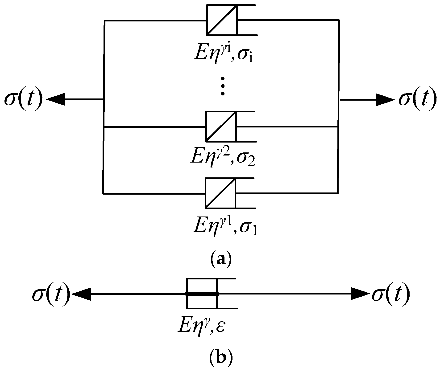
3.1. Establishment of the Distributed Order Damper

According to the fractional order theory, the constitutive equation of Abel dashpot could be expressed by Equation (12).

$$\sigma (t)=E{\eta }^{\gamma } {}_{0}D_t^{\gamma }[\epsilon (t)]\hspace{1em}(0\le \gamma \le 1)$$

(12)

When σ(t) = σ₀, the creep equation of Abel dashpot is as follows:

$$\epsilon (t)=\frac{{\sigma }_0}{E{\eta }^{\gamma }}\frac{t^{\beta }}{\Gamma (\beta +1)}\hspace{1em}(\beta \in R^{+},t>0)$$

(13)

The distributed order damper is made of many different fractional order dampers with various orders in parallel, as shown in Figure 1a. To facilitate the expression, Figure 1a can be simplified as Figure 1b.

Based on the single Abel damper and the series–parallel relationships, the stress–strain relationship of the distributed order damper could be expressed as follows:

$$\sigma (t)={\displaystyle \sum _{\mathrm{i}=1}^{n}E{\eta }^{{\gamma }_i} {}_{0}D_t^{\mathit{\gamma i}}[\epsilon (t)]}\hspace{1em}(0\le {\gamma }_{\mathrm{i}}\le 1)$$

(14)

The distributed order damper could be used with different orders to show the creep properties of anisotropic materials.

For Equation (14), suppose that $\Delta \gamma ={\gamma }_{\mathrm{i}}-{\gamma }_{\mathrm{i}-1}$, for $0\le a\le {\gamma }_{\mathrm{i}}\le b\le 1$, $[a,b]$ can be divided into $N=\frac{b-a}{\Delta \gamma }$, and Equation (15) could be obtained.

$$\sigma (t)={\displaystyle \sum _{\mathrm{i}=1}^{n}E{\eta }^{(i\Delta \gamma )} {}_{0}D_t^{i\Delta \gamma }[\epsilon (t)]}\hspace{1em}(0\le \gamma \le 1)$$

(15)

Let

$$\omega (i\Delta \gamma )=\frac{E{\eta }^{(i\Delta \gamma )}}{\Delta \gamma }$$

(16)

Suppose that Δγ was small enough, Equation (15) could be transformed into Equation (17).

$$\sigma (t)={\int }_a^b\omega (\gamma ) {}_{0}D_t^{\mathrm{(\gamma )}}[\epsilon (t)]d\gamma \hspace{1em}(0\le \gamma \le 1)$$

(17)

where ω(γ) is the kernel function of the distributed order derivative model.

In particular, for Equation (17), when ω(γ) is the impulse function, Equation (18) could be obtained.

$$\omega (\gamma )\delta (\gamma -{\gamma }_0)=0(\gamma \ne {\gamma }_0),\hspace{1em}{\int }_{-\infty }^{+\infty }\delta (\gamma -{\gamma }_0)d\gamma =1$$

(18)

According to the screening properties, Equation (19) could be obtained.

$${\int }_{-\infty }^{+\infty }\delta (\gamma -{\gamma }_0)f(\gamma )d\gamma =f({\gamma }_0)$$

(19)

By substituting Equations (18) and (19) into Equation (17), the following equation could be obtained.

$$\begin{array}{l}\sigma (t)={\displaystyle {\int }_a^b\delta (\gamma -{\gamma }_0){}_{0}D_t^{\gamma }[\epsilon (t)]}d\gamma \\ ={}_{0}D_t^{{\gamma }_0}[\epsilon (t)]\hspace{1em}(0\le \gamma \le 1)\end{array}$$

(20)

Therefore, when the kernel function is the impulse function, the distributed order model will change into the fractional order model.

3.2. Establishment of the Distributed Order Rheological Model and Operator Analysis

(1)

Establishment of the model

The three-parameter solid model is one of the essential models of viscoelastic materials. It is made of one spring and one Kelvin model in series, as shown in Figure 2a. It can be used to show instantaneous elastic deformation, deceleration creep deformation, and asymptotic creep deformation, as well as the relaxation properties of materials. With its advantages, it has been used to analyse the viscoelastic characteristics of many materials [28]. Therefore, the distributed order rheological model was established based on the three-parameter solid model. The damper components in the integer-order model were changed into the distributed order damper, as shown in Figure 1b. Thus, the distributed order three-parameter solid model was obtained, as shown in Figure 2b.

According to the stress–strain relationships of the components and the series–parallel relationships among the components, the three-parameter solid model equation of state could be expressed by Equation (21).

$$\{\begin{array}{l}\sigma (t)=E_1{\epsilon }_1(t), {\sigma }_1(t)=E_2{\epsilon }_2(t), {\sigma }_2(t)={\displaystyle {\int }_a^b\omega (\gamma ){}_{0}D_t^{\gamma }[{\epsilon }_2(t)]}d\gamma \\ \epsilon (t)={\epsilon }_1(t)+{\epsilon }_2(t), \sigma (t)={\sigma }_1(t)+{\sigma }_2(t)\end{array}$$

(21)

By Equation (21), the constitutive equation of the distributed order three-parameter solid model could be obtained as follows:

$$\begin{array}{l}{\displaystyle {\int }_a^b\omega (\gamma ){}_{0}D_t^{\gamma }[\sigma (t)]}d\gamma +(E_1+E_2)\sigma (t)\\ =E_1{\displaystyle {\int }_a^b\omega (\gamma ){}_{0}D_t^{\gamma }[\epsilon (t)]}d\gamma +E_1{E}_2\epsilon (t)\\ \end{array}$$

(22)

Let ν = E₁ + E₂ and κ = E₁E₂, Equation (22) could be changed into Equation (23).

$$\begin{array}{l}{\displaystyle {\int }_a^b\omega (\gamma ){}_{0}D_t^{\gamma }[\sigma (t)]}d\gamma +\nu \sigma (t)=\\ E_1{\displaystyle {\int }_a^b\omega (\gamma ){}_{0}D_t^{\gamma }[\epsilon (t)]}d\gamma +\kappa \epsilon (t)\end{array}$$

(23)

where E₁ > 0, κ > 0, ν > 0, and E₁ν-κ ≥ 0. The parameter values depend on the properties of the materials.

Equation (23) could be changed into Equation (24) by the Laplace transform.

$$\nu \sigma (s)+{\int }_a^b\omega (\gamma )s^{\gamma }d\gamma \sigma (s)=E_1{\int }_a^b\omega (\gamma )s^{\gamma }d\gamma \epsilon (s)+\kappa \epsilon (s)$$

(24)

On this basis, Equation (25) could be obtained.

$$\sigma (s)=\frac{E_1{\displaystyle {\int }_a^b\omega (\gamma )s^{\gamma }}d\gamma +\kappa }{\nu +{\displaystyle {\int }_a^b\omega (\gamma )s^{\gamma }}d\gamma }\epsilon (s)$$

(25)

Thus, the creep compliance of the distributed order three-parameter solid model could be obtained.

$$\begin{array}{l}J(t)=L^{-1}\left\{J(s)\right\}=L^{-1}\left\{\frac{\epsilon (s)}{s\sigma (s)}\right\}\\ =L^{-1}\left\{\frac{1}{E_{1}s}+\frac{E_1\nu -\kappa }{s{E}_1^2}\frac{1}{{\displaystyle {\int }_a^b\omega (\gamma )s^{\gamma }}d\gamma +\frac{\kappa }{E_1}}\right\}\end{array}$$

(26)

Similarly, the relaxation modulus of the distributed order three-parameter solid model could be calculated.

$$\begin{array}{l}G(t)=L^{-1}\left\{G(s)\right\}=L^{-1}\left\{\frac{\sigma (s)}{s\epsilon (s)}\right\}\\ =L^{-1}\left\{\frac{E_1}{s}+\frac{\kappa -E_1\lambda }{\nu +{\displaystyle {\int }_a^b\omega (\gamma )s^{\gamma }}d\gamma }\frac{1}{s}\right\}\end{array}$$

(27)

The inverse Laplace transform of $\frac{1}{\nu +{\displaystyle {\int }_a^b\omega (\gamma )s^{\gamma }}d\gamma }$ could be obtained by calculating Equations (26) and (27).

(2)

Properties of model operators

Let

$$\tilde{f}(s)=\frac{1}{\nu +{\displaystyle {\int }_a^b\omega (\gamma )s^{\gamma }}d\gamma }\hspace{1em}(\tilde{f}\to f:s\to t)$$

(28)

Equation (29) could be obtained by the inverse Laplace transform of Equation (28).

$$\begin{array}{l}f(t)=L^{-1}\left[\frac{1}{\nu +{\displaystyle {\int }_a^b\omega (\gamma )s^{\gamma }}d\gamma }\right]=\\ \frac{1}{2\pi i}{\displaystyle {\int }_{\delta -i\infty }^{\delta +i\infty }\frac{e^{st}}{\nu +{\displaystyle {\int }_a^b\omega (\gamma )s^{\gamma }}d\gamma }ds}\hspace{1em}(\delta >0)\end{array}$$

(29)

where the critical path of Equation (29) is shown in Figure 3.

The premise for the calculation of Equation (29) was to judge whether the operator $\tilde{f}(s)$ had poles, that is, points whose denominators were zero. Suppose that there were poles in the integral domain of $\Omega =\{s\in c:0<r<\left|s\right|<R,\left|Arg(s)\right|<\pi \}$, Equation (30) could be calculated.

$$s=x{e}^{i\theta },\hspace{0.5em}\theta \in (-\pi ,\pi )$$

(30)

where x and θ are variables.

By substituting Equation (30) into the denominator in Equation (28), Equation (31) could be obtained.

$$\begin{array}{l}\nu +{\displaystyle {\int }_a^b\omega (\gamma )s^{\gamma }}d\gamma =\nu +{\displaystyle {\int }_a^b\omega (\gamma )x^{\gamma }{e}^{i\theta \gamma }}d\gamma \\ =\nu +{\displaystyle {\int }_a^b\omega (\gamma )x^{\gamma }\cos (\theta \gamma )}d\gamma +i{\displaystyle {\int }_a^b\omega (\gamma )x^{\gamma }\sin (\theta \gamma )}d\gamma =0\end{array}$$

(31)

According to the assumption, Equation (32) could be obtained.

$$\{\begin{array}{l}\nu +{\displaystyle {\int }_a^b\omega (\gamma )x^{\gamma }\cos (\theta \gamma )}d\gamma =0\\ {\displaystyle {\int }_a^b\omega (\gamma )x^{\gamma }\sin (\theta \gamma )}d\gamma =0\end{array}$$

(32)

For Equation (32), when 0 ≤ γ ≤ 1, 0 ≤ θγ ≤ π and 0 ≤ sin (θγ) ≤ 1. Only when θγ = kπ and k was an integer, sin (θγ) = 0. However, θ $\in$ (−π,π), so k could not be an integer. On the other hand, ν > 0, Equation (29) was not valid. Therefore, the operator $\tilde{f}(s)$ had no poles in the area of $\Omega =\{s\in c:0<r<\left|s\right|<R,\left|Arg(s)\right|<\pi \}$.

Next, the complex plane was cut. Equation (29) could be calculated by converting the contour integral into Hankel’s integrals. According to the definition of a fulcrum, the operator $\tilde{f}(s)$ had two fulcrums, that is, s = 0 and s = ∞. The complex plane was cut along the negative real axis to obtain the single-valued branch. The contour integral (Figure 3) was converted into the Hankel integral path (Figure 4).

Let $s=x{e}^{-i\pi },x\in (0,\infty )$ in the secant of a lower branch, Equation (33) could be obtained along the path of the Hankel integral.

$$f_1(t)=\frac{1}{2\pi i}{\int }_0^{\infty }\frac{e^{-xt}}{\nu +{\int }_a^b\omega (\gamma )x^{\gamma }{e}^{-i\pi \gamma }d\gamma }dx$$

(33)

Let $s=x{e}^{i\pi },x\in (0,\infty )$ in the secant of an upper branch, Equation (34) could be obtained.

$$f_2(t)=\frac{1}{2\pi i}{\int }_0^{\infty }\frac{e^{-xt}}{\nu +{\int }_a^b\omega (\gamma )x^{\gamma }{e}^{i\pi \gamma }d\gamma }dx$$

(34)

For Equations (33) and (34), the path integral of Hankel was 0 along a small circular path with a radius r of 0. Equation (35) could be obtained.

$$\begin{array}{l}f(t)=L^{-1}\left[\frac{1}{\nu +{\int }_a^b\omega (\gamma )s^{\gamma }d\gamma }\right]=f_1(t)-f_2(t)\\ =\frac{1}{2\pi i}{\int }_0^{\infty }\frac{e^{-xt}}{\nu +{\int }_a^b\omega (\gamma )x^{\gamma }{e}^{-i\pi \gamma }d\gamma }dx-\frac{1}{2\pi i}{\int }_0^{\infty }\frac{e^{-xt}}{\nu +{\int }_a^b\omega (\gamma )x^{\gamma }{e}^{i\pi \gamma }d\gamma }dx\\ =\frac{1}{2\pi i}{\int }_0^{\infty }\frac{e^{-xt}}{\nu +{\int }_a^b\omega (\gamma )x^{\gamma }\cos (\pi \gamma )d\gamma -i{\int }_a^b\omega (\gamma )x^{\gamma }\sin (\pi \gamma )d\gamma }dx\\ -\frac{1}{2\pi i}{\int }_0^{\infty }\frac{e^{-xt}}{\nu +{\int }_a^b\omega (\gamma )x^{\gamma }\cos (\pi \gamma )d\gamma +i{\int }_a^b\omega (\gamma )x^{\gamma }\sin (\pi \gamma )d\gamma }dx\\ =\frac{1}{2\pi i}{\int }_0^{\infty }\frac{e^{-xt}2i{\int }_a^b\omega (\gamma )x^{\gamma }\sin (\pi \gamma )d\gamma }{{(\nu +{\int }_a^b\omega (\gamma )x^{\gamma }\cos (\pi \gamma )d\gamma )}^2+{({\int }_a^b\omega (\gamma )x^{\gamma }\sin (\pi \gamma )d\gamma )}^2}dx\\ =\frac{1}{\pi }{\int }_0^{\infty }\frac{e^{-xt}{\int }_a^b\omega (\gamma )x^{\gamma }\sin (\pi \gamma )d\gamma }{{[\nu +{\int }_a^b\omega (\gamma )x^{\gamma }\cos (\pi \gamma )d\gamma ]}^2+{[{\int }_a^b\omega (\gamma )x^{\gamma }\sin (\pi \gamma )d\gamma ]}^2}dx\end{array}$$

(35)

f(t) was an utterly monotone function, so the upper boundary could be obtained for arbitrary $t\in [0,\infty )$, ${(-1)}^n{[f(t)]}^{(n)}\ge 0$, according to the time-domain expression.

$$\begin{array}{l}f(t)=\frac{1}{\pi }{\int }_0^{\infty }\frac{e^{-xt}{\int }_a^b\omega (\gamma )x^{\gamma }\sin (\pi \gamma )d\gamma }{{[\nu +{\int }_a^b\omega (\gamma )x^{\gamma }\cos (\pi \gamma )d\gamma ]}^2+{[{\int }_a^b\omega (\gamma )x^{\gamma }\sin (\pi \gamma )d\gamma ]}^2}dx\\ \le \frac{1}{\pi }{\int }_0^{\infty }\frac{e^{-xt}{\int }_a^b\omega (\gamma )x^{\gamma }\sin (\pi \gamma )d\gamma }{{[{\int }_a^b\omega (\gamma )x^{\gamma }\sin (\pi \gamma )d\gamma ]}^2}dx=\frac{1}{\pi }{\int }_0^{\infty }\frac{e^{-xt}}{{\int }_a^b\omega (\gamma )x^{\gamma }\sin (\pi \gamma )d\gamma }dx\\ =\frac{1}{\pi }{\int }_0^{\infty }\frac{e^{-xt}}{\omega (\widehat{\gamma })x^{\widehat{\gamma }}\sin (\pi \widehat{\gamma })(b-a)}dx\\ =\frac{1}{\pi }\frac{t^{\widehat{\gamma }-1}}{\omega (\widehat{\gamma })\sin (\pi \widehat{\gamma })(b-a)}{\int }_0^{\infty }{e}^{-xt}{(tx)}^{-\widehat{\gamma }}d(xt)\\ =\frac{1}{\pi }\frac{t^{\widehat{\gamma }-1}}{\omega (\widehat{\gamma })\sin (\pi \widehat{\gamma })(b-a)}\Gamma (1-\widehat{\gamma })\le \frac{1}{\pi }\frac{t^{b-1}}{\omega (\widehat{\gamma })\sin (\pi \widehat{\gamma })(b-a)}\Gamma (1-\widehat{\gamma })\hspace{1em}\hspace{1em}\widehat{\gamma }\in (a,b)\end{array}$$

(36)

Similarly, the lower boundary could be obtained as follows:

$$\begin{array}{l}f(t)=\frac{1}{\pi }{\int }_0^{\infty }\frac{e^{-xt}{\int }_a^b\omega (\gamma )x^{\gamma }\sin (\pi \gamma )d\gamma }{{[\nu +{\int }_a^b\omega (\gamma )x^{\gamma }\cos (\pi \gamma )d\gamma ]}^2+{[{\int }_a^b\omega (\gamma )x^{\gamma }\sin (\pi \gamma )d\gamma ]}^2}dx\\ \ge \frac{1}{\pi }{\int }_0^{\infty }\frac{e^{-xt}{\int }_a^b\omega (\gamma )x^{\gamma }\sin (\pi \gamma )d\gamma }{{[\nu +{\int }_a^b\omega (\gamma )x^{\gamma }d\gamma ]}^2+{[{\int }_a^b\omega (\gamma )x^{\gamma }d\gamma ]}^2}dx\\ =\frac{1}{\pi }{\int }_0^{\infty }\frac{e^{-xt}{x}^{\tilde{\gamma }}\omega (\tilde{\gamma })\sin (\pi \tilde{\gamma })(b-a)}{2{[\nu +{\int }_a^b\omega (\gamma )x^{\gamma }d\gamma ]}^2}dx\\ =\frac{1}{\pi }\frac{\omega (\tilde{\gamma })\sin (\pi \tilde{\gamma })(b-a)}{2{[\nu +\omega (\tilde{\gamma }){\overline{x}}^a]}^2}{\int }_0^{\infty }{e}^{-xt}{x}^{\tilde{\gamma }}dx\\ =\frac{1}{\pi }\frac{\omega (\tilde{\gamma })\sin (\pi \tilde{\gamma })(b-a)}{2{[\nu +\omega (\tilde{\gamma }){\overline{x}}^a]}^2}{t}^{-1-\tilde{\gamma }}\Gamma (1+\tilde{\gamma })\\ \ge \frac{1}{\pi }\frac{\omega (\tilde{\gamma })\sin (\pi \tilde{\gamma })(b-a)}{2{[\nu +\omega (\tilde{\gamma }){\overline{x}}^a]}^2}{t}^{-1-a}\Gamma (1+\tilde{\gamma })\hspace{1em}\hspace{1em}\hspace{0.5em}\tilde{\gamma }\in (a,b),\overline{x}\in (0,\infty )\end{array}$$

(37)

A calculation example: With ν = 0.1, a = 0.3, b = 0.8, ω(γ) = 1 and $\widehat{\gamma }=0.6,\tilde{\gamma }=0.5,\overline{x}=0.5$, the analytic values, upper boundary, and lower boundary values of f(t) could be calculated, as shown in Figure 5.

3.3. Response Characteristics of the Rheological Properties of the Distributed Order Rheological Model

According to the above calculation process, we can directly calculate the creep compliance and relaxation modulus of the distributed order three-parameter solid model (Figure 2).

By substituting Equation (35) into Equation (26), the creep compliance could be obtained as follows:

$$J(t)=\frac{1}{E_1}+\frac{E_1\nu -\kappa }{E_1^2}{\int }_0^{\infty }\frac{1}{\pi }\frac{1-e^{-xt}}{x}\frac{{\int }_a^b\omega (\gamma )x^{\gamma }\sin (\pi \gamma )d\gamma }{{[\frac{\kappa }{E_1}+{\int }_a^b\omega (\gamma )x^{\gamma }\cos (\pi \gamma )d\gamma ]}^2+{[{\int }_a^b\omega (\gamma )x^{\gamma }\sin (\pi \gamma )d\gamma ]}^2}dx$$

(38)

The relaxation modulus could be calculated by substituting Equation (35) into Equation (27).

$$G(t)=E_1-{\int }_0^{\infty }\frac{E_1\nu -\kappa }{\pi }\frac{1-e^{-xt}}{x}\frac{{\int }_a^b\omega (\gamma )x^{\gamma }\sin (\pi \gamma )d\gamma }{{[\lambda +{\int }_a^b\omega (\gamma )x^{\gamma }\cos (\pi \gamma )d\gamma ]}^2+{[{\int }_a^b\omega (\gamma )x^{\gamma }\sin (\pi \gamma )d\gamma ]}^2}dx$$

(39)

A calculation example: With ν = 0.1, a = 0.3, b = 0.8, ω(γ) = 1, E₁ = 2, and κ = 0.03, we could obtain the creep response and relaxation response of the distributed order three-parameter solid model, as shown in Figure 6.

In Figure 6, as time went by, the creep compliance increased gradually, and the velocity of increase gradually decreased and finally tended to a specific value, which could present the properties of the viscoelastic materials at the deceleration creep stage and sound creep stage. The relaxation modulus and the change rate decreased gradually and finally tended to a specific value, which could better show the relaxation characteristics of the viscoelastic materials.

4. The Distributed Order Damage Creep Model of Rock Mass

Compared with viscoelastic materials, rock materials have both viscoelastic characteristics and great plastic deformation during the creep deformation process. The experimental results of rock creep indicated that when the stress was immense, the rock mass experienced a prominent accelerated creep stage, which was the plastic deformation caused by the internal damage accumulation. Therefore, the established damage model should reflect the damage characteristics of the rock mass [48,49].

4.1. Establishment and Properties of the Distributed Order Damper Damage Model

(1)

Establishment of the distributed order damper damage model

According to the fractional order theory, the fractional order damper damage model was constructed to show accelerated rock deformation, and the constitutive relation could be expressed by Equation (40).

$$\sigma (t)=E{\eta }^{\gamma }{e}^{-\lambda t}{}_{0}D_t^{\gamma }[\epsilon (t)]\hspace{1em}(0\le \gamma \le 1)$$

(40)

where $E{\eta }^{\gamma }{e}^{-\lambda t}$ denotes the time-dependent viscosity coefficient and λ denotes the damage factor. By the Laplace transform, Equation (41) can be expressed:

$$\epsilon (s+\lambda )=\frac{\sigma (s)}{E{\eta }^{\gamma }{(s+\lambda )}^{\gamma }},\hspace{1em}0\le \gamma \le 1$$

(41)

To show the anisotropy of the rock mass, multiple fractional order damage dampers with various orders were connected in series, as shown in Figure 7.

According to the calculation methods of the component series, Equation (42) could be obtained.

$$\epsilon (s+\lambda )=\sum _{i=1}^n{\epsilon }_i(s+\lambda )=\sum _{i=1}^n\frac{\sigma (s)}{E{\eta }^{{\gamma }_i}{(s+\lambda )}^{{\gamma }_i}},0\le \gamma \le 1$$

(42)

With the same method and the assumption that $\Delta \gamma$ was small enough, for $0\le a\le {\gamma }_{\mathrm{i}}\le b\le 1$, $[a,b]$ could be converted into $N=\frac{b-a}{\Delta \gamma }$, and Equation (42) could be transformed into Equation (43).

$$\epsilon (s+\lambda )=\sum _{i=1}^n\frac{\sigma (s)}{E{\eta }^{(i\Delta \gamma )}{(s+\lambda )}^{(i\Delta \gamma )}}$$

(43)

According to the definition of the definite integral, Equation (44) could be obtained.

$$\epsilon (s+\lambda )={\int }_a^b\frac{\omega (\gamma )}{{(s+\lambda )}^{\gamma }}d\gamma \sigma (s)$$

(44)

Specifically, when $\omega (\gamma )$ is the impulse function, Equation (44) could be changed into Equation (45).

$$\epsilon (s+\lambda )={\int }_a^b\frac{\delta (\gamma -{\gamma }_0)}{{(s+\lambda )}^{\gamma }}d\gamma =\frac{1}{{(s+\lambda )}^{{\gamma }_0}}\sigma (s)$$

(45)

By the inverse Laplace transform, Equation (45) could be converted into Equation (46).

$$\sigma (t)=e^{-\lambda t}{}_{0}D_t^{{\gamma }_0}[\epsilon (t)]$$

(46)

This was the fractional order damage damper.

By the inverse Laplace transform of Equation (44), Equation (47) could be obtained.

$$\epsilon (t)=e^{\lambda t}{L}^{-1}\left\{{\int }_a^b\frac{\omega (\gamma )}{{(s+\lambda )}^{\gamma }}d\gamma \sigma (s)\right\},\hspace{1em}0\le \gamma \le 1$$

(47)

With N harmonics, the Fourier series approximation of $\omega (\gamma )$ in Equation (47) was expressed by Equation (48).

$$\omega (\gamma )=\frac{a_0}{2}+\sum _{n=1}^N[a_n\cos ({\tau }_n\gamma )+b_n\sin ({\tau }_n\gamma )]$$

(48)

where

$$\{\begin{array}{l}{a}_n=\frac{2}{b-a}{\int }_a^b\omega (\gamma )\cos ({\tau }_n\gamma )d\gamma \\ b_n=\frac{2}{b-a}{\int }_a^b\omega (\gamma )\sin ({\tau }_n\gamma )d\gamma \\ {\tau }_n=\frac{2n\pi }{b-a}\end{array}\hspace{1em}n=0,1,2,\cdots ,N$$

(49)

By further calculation, Equation (50) could be obtained.

$$\begin{array}{cc}\epsilon (t)& =e^{\lambda t}{L}^{-1}\left\{{\int }_a^b\frac{\omega (\gamma )}{{(s+\lambda )}^{\gamma }}d\gamma \sigma (s)\right\}\\ & =e^{\lambda t}{L}^{-1}\left\{{\int }_a^b\left\{\frac{a_0}{2}+{\displaystyle \sum _{n=1}^N}[a_n\cos ({\tau }_n\gamma )+b_n\sin ({\tau }_n\gamma )]\right\}\frac{1}{{(s+\lambda )}^{\gamma }}d\gamma \sigma (s)\right\}\end{array}$$

(50)

Equation (50) could be solved by the inverse Laplace transform of ${\int }_a^b\frac{\omega (\gamma )}{{(s+\lambda )}^{\gamma }}d\gamma$.

(2)

Properties of operators

(i)

Properties of ${\int }_a^b\frac{1}{{(s+\lambda )}^{\gamma }}d\gamma$

Let

$${\tilde{g}}_1(s)={\int }_a^b\frac{1}{{(s+\lambda )}^{\gamma }}d\gamma$$

(51)

$${\tilde{g}}_2(s)={\int }_a^b\frac{1}{s^{\gamma }}d\gamma =\frac{s^{-a}-s^{-b}}{\ln (s)}$$

(52)

Then

$$g_1(t)=L^{-1}\left\{{\int }_a^b\frac{1}{{(s+\lambda )}^{\gamma }}d\gamma \right\}=e^{-\lambda t}\left\{{\int }_a^b\frac{1}{s^{\gamma }}d\gamma \right\}=e^{-\lambda t}{g}_2(t)$$

(53)

By the inverse Laplace transform of Equation (52):

$$\begin{array}{l}{g}_2(t)=L^{-1}\left\{{\tilde{g}}_2(s)\right\}\\ =\frac{1}{2\pi i}{\int }_{\delta -i\pi }^{\delta +i\pi }{e}^{st}{\int }_a^b{s}^{-\gamma }d\gamma ds\\ =\frac{1}{2\pi i}{\int }_{\delta -i\pi }^{\delta +i\pi }{e}^{st}\frac{\ln (s)}{s^{-a}-s^{-b}}ds\end{array}$$

(54)

Obviously, ${\tilde{g}}_2(s)$ had no poles in the area of $\Omega =\{s\in c:0<r<\left|s\right|<R,\left|Arg(s)\right|<\pi \}$. ${\tilde{g}}_2(s)$ had two fulcrums, that is, $s=0$ and $s=\infty$. The single-valued branch could be obtained after cutting the complex plane along the negative real axis. The radiation angle was $Arg(s)\in (-\pi ,\pi )$. The contour integral (Figure 3) was transformed into the path of the Hankel integral (Figure 4). Equation (55) could be obtained through the calculation along the Hankel path.

$$\begin{array}{l}{g}_2(t)=L^{-1}\left\{{\int }_a^b\frac{1}{s^{\gamma }}d\gamma \right\}=\frac{1}{2\pi i}{\int }_{\delta -i\pi }^{\delta +i\pi }{e}^{st}\frac{s^{-a}-s^{-b}}{\ln (s)}ds\\ =\frac{1}{2\pi i}{\int }_0^{\infty }{e}^{-xt}\frac{x^{-a}{e}^{a\pi i}-x^{-b}{e}^{b\pi i}}{\ln (x)-i\pi }dx-\frac{1}{2\pi i}{\int }_0^{\infty }{e}^{-xt}\frac{x^{-a}{e}^{-a\pi i}-x^{-b}{e}^{-b\pi i}}{\ln (x)+i\pi }dx\\ =\frac{1}{2\pi i}{\int }_0^{\infty }{e}^{-xt}\frac{(x^{-a}{e}^{a\pi i}-x^{-b}{e}^{b\pi i})(\ln (x)+i\pi )}{{\ln }^2(x)+{\pi }^2}-\frac{(x^{-a}{e}^{-a\pi i}-x^{-b}{e}^{-b\pi i})(\ln (x)-i\pi )}{{\ln }^2(x)+{\pi }^2}dx\\ =\frac{1}{2\pi i}{\int }_0^{\infty }{e}^{-xt}\frac{(x^{-a}{e}^{a\pi i}-x^{-b}{e}^{b\pi i})\ln (x)+i\pi (x^{-a}{e}^{a\pi i}-x^{-b}{e}^{b\pi i})-\ln (x)(x^{-a}{e}^{-a\pi i}-x^{-b}{e}^{-b\pi i})-i\pi (x^{-a}{e}^{-a\pi i}-x^{-b}{e}^{-b\pi i})}{{\ln }^2(x)+{\pi }^2}dx\\ =\frac{1}{2\pi i}{\int }_0^{\infty }{e}^{-xt}\frac{\ln (x)x^{-a}(e^{a\pi i}-e^{-a\pi i})+i\pi x^{-a}(e^{a\pi i}+e^{-a\pi i})-\ln (x)x^{-b}(e^{b\pi i}-e^{-b\pi i})-i\pi x^{-b}(e^{-b\pi i}+e^{b\pi i})}{{\ln }^2(x)+{\pi }^2}dx\\ =\frac{1}{\pi }{\int }_0^{\infty }\frac{e^{-xt}}{{\ln }^2(x)+{\pi }^2}[x^{-a}(\sin (a\pi )\ln (x)+\pi \cos (a\pi ))-x^{-b}(\sin (b\pi )\ln (x)+\pi \cos (b\pi ))]dx\end{array}$$

(55)

Meanwhile, Equation (56) could be obtained.

$$\begin{array}{l}{g}_2(t)=L^{-1}\left\{{\int }_a^b\frac{1}{s^{\gamma }}d\gamma \right\}=\frac{1}{2\pi i}{\int }_{\delta -i\pi }^{\delta +i\pi }{e}^{st}{s}^{-\gamma }ds\\ =\frac{1}{2\pi i}{\int }_0^{\infty }{e}^{-xt}{\int }_a^b{(x{e}^{-\pi i})}^{-\gamma }d\gamma dx-\frac{1}{2\pi i}{\int }_0^{\infty }{e}^{-xt}{\int }_a^b{(x{e}^{\pi i})}^{-\gamma }d\gamma dx\\ =\frac{1}{2\pi i}{\int }_0^{\infty }{e}^{-xt}{\int }_a^{b}2i{x}^{-\gamma }\sin (\pi \gamma )d\gamma dx=\frac{1}{\pi }{\int }_0^{\infty }{e}^{-xt}{\int }_a^b{x}^{-\gamma }\sin (\pi \gamma )d\gamma dx\end{array}$$

(56)

The asymptotic form of Equation (56) could be expressed as follows:

$$\begin{array}{l}\left|g_2(t)\right|=\left|\frac{1}{\pi }{\int }_0^{\infty }{e}^{-xt}{\int }_a^b{x}^{-\gamma }\sin (\pi \gamma )d\gamma dx\right|\le \frac{1}{\pi }{\int }_0^{\infty }{e}^{-xt}{\int }_a^b{x}^{-\gamma }d\gamma dx\\ \le \frac{b-a}{\pi }{\int }_0^1{e}^{-xt}{x}^{-b}dx+\frac{b-a}{\pi }{\int }_1^{\infty }{e}^{-xt}{x}^{-a}dx\\ \le \frac{b-a}{\pi }{t}^{b-1}\Gamma (1-b)+\frac{b-a}{\pi }{t}^{a-1}\Gamma (1-a)\end{array}$$

(57)

Furthermore, Equation (58) could be obtained.

$$\begin{array}{l}{g}_1(t)=L^{-1}\left\{{\int }_a^b\frac{1}{{(s+\lambda )}^{\gamma }}d\gamma \right\}=e^{-\lambda t}\left\{{\int }_a^b\frac{1}{s^{\gamma }}d\gamma \right\}\\ =\frac{1}{\pi }{\int }_0^{\infty }{e}^{-(x+\lambda )t}{\int }_a^b{x}^{-\gamma }\sin (\pi \gamma )d\gamma dx\\ =\frac{1}{\pi }{\int }_0^{\infty }\frac{e^{-(x+\lambda )t}}{{\ln }^2(x)+{\pi }^2}[x^{-a}(\sin (a\pi )\ln (x)+\pi \cos (a\pi ))-x^{-b}(\sin (b\pi )\ln (x)+\pi \cos (b\pi ))]dx\end{array}$$

(58)

The asymptotic form of Equation (58) could be expressed by Equation (59).

$$\begin{array}{l}\left|g_1(t)\right|=L^{-1}\left\{{\int }_a^b\frac{1}{{(s+\lambda )}^{\gamma }}d\gamma \right\}\\ =\frac{1}{\pi }{e}^{-\lambda t}{\int }_0^{\infty }{e}^{-xt}{\int }_a^b{x}^{-\gamma }\sin (\pi \gamma )d\gamma dx\le \frac{1}{\pi }{e}^{-\lambda t}{\int }_0^{\infty }{e}^{-xt}{\int }_a^b{x}^{-\gamma }d\gamma dx\\ \le \frac{b-a}{\pi }{e}^{-\lambda t}{\int }_0^1{e}^{-xt}{x}^{-b}dx+\frac{b-a}{\pi }{e}^{-\lambda t}{\int }_1^{\infty }{e}^{-xt}{x}^{-a}dx\\ \le \frac{b-a}{\pi }{e}^{-\lambda t}{t}^{b-1}\Gamma (1-b)+\frac{b-a}{\pi }{e}^{-\lambda t}{t}^{a-1}\Gamma (1-a)\end{array}$$

(59)

(ii)

Properties analysis of the operator ${\int }_a^b\frac{\omega (\gamma )}{{(s+\lambda )}^{\gamma }}d\gamma$

Let

$${\tilde{g}}_0(s)={\int }_a^b\frac{\omega (\gamma )}{{(s+\lambda )}^{\gamma }}d\gamma$$

(60)

Equation (60) could be obtained according to the above calculation method.

$$\begin{array}{cc}{g}_0(t)& =L^{-1}\left\{{\int }_a^b\omega (\gamma )\frac{1}{{(s+\lambda )}^{\gamma }}d\gamma \right\}\\ & =\frac{1}{\pi }{\int }_0^{\infty }{e}^{-(x+\lambda )t}{\int }_a^b\left\{\frac{a_0}{2}+{\displaystyle \sum _{n=1}^N}{a}_n\cos ({\tau }_n\gamma )+b_n\sin ({\tau }_n\gamma )\right\}{x}^{-\gamma }\sin (\pi \gamma )d\gamma dx\\ & =\frac{a_0}{2}\frac{1}{\pi }{\int }_0^{\infty }{e}^{-(x+\lambda )t}{\int }_a^b{x}^{-\gamma }\sin (\pi \gamma )dxd\gamma \\ & +\frac{1}{\pi }{\displaystyle \sum _{n=1}^N}\sqrt{a_n^2+b_n^2}{\int }_0^{\infty }{e}^{-(x+\lambda )t}{\int }_a^b\sin ({\varphi }_n+{\tau }_n\gamma )x^{-\gamma }\sin (\pi \gamma )dxd\gamma \end{array}$$

(61)

The corresponding asymptotic properties are given as follows:

$$\begin{array}{l}\left|g_0(t)\right|=\left|L^{-1}\left\{{\int }_a^b\frac{\omega (\gamma )}{{(s+\lambda )}^{\gamma }}d\gamma \right\}\right|\\ =\left|\frac{1}{\pi }{\int }_0^{\infty }{e}^{-(x+\lambda )t}{\int }_a^b\left\{\frac{a_0}{2}+{\displaystyle \sum _{n=1}^N}\sqrt{a_n^2+b_n^2}\sin ({\varphi }_n+{\tau }_n\gamma )\right\}{x}^{-\gamma }\sin (\pi \gamma )dxd\gamma \right|\\ \le \frac{1}{\pi }{\int }_0^{\infty }{e}^{-(x+\lambda )t}{\int }_a^b\left(\frac{a_0}{2}+{\displaystyle \sum _{n=1}^N}\sqrt{a_n^2+b_n^2}\right)x^{-\gamma }d\gamma dx\\ \le \frac{1}{\pi }\sqrt{(N+\frac{1}{2})[\frac{a_{{}_0}^2}{2}+{\displaystyle \sum _{n=1}^N}(a_n^2+b_n^2)]}{\int }_0^{\infty }{e}^{-(x+\lambda )t}{\int }_a^b{x}^{-\gamma }d\gamma dx\\ =\frac{1}{\pi }\sqrt{(N+\frac{1}{2}){\int }_a^b{\omega }^2(\gamma )d\gamma }{\int }_0^{\infty }{e}^{-(x+\lambda )t}{\int }_a^b{x}^{-\gamma }d\gamma dx\\ \le \sqrt{(N+\frac{1}{2}){\int }_a^b{\omega }^2(\gamma )d\gamma }\frac{b-a}{\pi }{e}^{-\lambda t}{\int }_0^1{e}^{-xt}{x}^{-b}dx+\sqrt{(N+\frac{1}{2}){\int }_a^b{\omega }^2(\gamma )d\gamma }\frac{b-a}{\pi }{e}^{-\lambda t}{\int }_1^{\infty }{e}^{-xt}{x}^{-a}dx\\ \le \sqrt{(N+\frac{1}{2}){\int }_a^b{\omega }^2(\gamma )d\gamma }\frac{b-a}{\pi }{e}^{-\lambda t}{t}^{b-1}\Gamma (1-b)+\sqrt{(N+\frac{1}{2}){\int }_a^b{\omega }^2(\gamma )d\gamma }\frac{b-a}{\pi }{e}^{-\lambda t}{t}^{a-1}\Gamma (1-a)\end{array}$$

(62)

(3)

Creep response of the distributed order damage damper

When $\sigma (t)={\sigma }_0$,$\sigma (s)=\frac{{\sigma }_0}{s}$, Equation (50) could be changed into Equation (63).

$$\epsilon (t)=e^{\lambda t}{L}^{-1}\left\{{\int }_a^b\left\{\frac{a_0}{2}+\sum _{n=1}^N[a_n\cos ({\tau }_n\gamma )+b_n\sin ({\tau }_n\gamma )]\right\}\frac{1}{{(s+\lambda )}^{\gamma }}d\gamma \frac{{\sigma }_0}{s}\right\} (0\le \gamma \le 1)$$

(63)

In fact,

$$\begin{array}{l}{L}^{-1}\left\{\frac{{\sigma }_0}{s}\right\}\ast L^{-1}\left\{{\int }_a^b\frac{\omega (\gamma )}{{(s+\lambda )}^{\gamma }}d\gamma \right\}\\ =\frac{{\sigma }_0}{\pi }{\int }_0^t{\int }_0^{\infty }{e}^{-(x+\lambda )(t-\tau )}\left\{\frac{a_0}{2}+{\displaystyle \sum _{n=1}^N[a_n\cos ({\tau }_n\gamma )+b_n\sin ({\tau }_n\gamma )]}\right\}{\int }_a^b{x}^{-\gamma }\sin (\pi \gamma )d\gamma dxd\tau \\ =\frac{{\sigma }_0}{\pi }{\int }_0^t{\int }_0^{\infty }{e}^{-(x+\lambda )t}{e}^{(x+\lambda )\tau }\left\{\frac{a_0}{2}+{\displaystyle \sum _{n=1}^N\sqrt{a_n^2+b_n^2}}\sin ({\varphi }_n+{\tau }_n\gamma )\right\}{\int }_a^b{x}^{-\gamma }\sin (\pi \gamma )d\gamma dxd\tau \\ =\frac{{\sigma }_0}{\pi }{\int }_0^{\infty }\frac{1-e^{-(x+\lambda )t}}{x+\lambda }\frac{1}{{\ln }^2(x)+{\pi }^2}\left\{\frac{a_0}{2}+{\displaystyle \sum _{n=1}^N\sqrt{a_n^2+b_n^2}}\sin ({\varphi }_n+{\tau }_n\gamma )\right\}{\int }_a^b{x}^{-\gamma }\sin (\pi \gamma )d\gamma dx\end{array}$$

(64)

Through further calculation, Equation (65) could be obtained.

$$\begin{array}{l}\epsilon (t)=e^{\lambda t}\left\{L^{-1}\left\{\frac{{\sigma }_0}{s}\right\}\ast L^{-1}\left\{{\int }_a^b\frac{\omega (\gamma )}{{(s+\lambda )}^{\gamma }}d\gamma \right\}\right\}\\ =\frac{{\sigma }_0}{\pi }{\int }_0^{\infty }\frac{e^{\lambda t}-e^{-xt}}{x+\lambda }{\int }_a^b\left\{\frac{a_0}{2}+{\displaystyle \sum _{n=1}^N[a_n\cos ({\tau }_n\gamma )+b_n\sin ({\tau }_n\gamma )]}\right\}{x}^{-\gamma }\sin (\pi \gamma )d\gamma dx\\ =\frac{{\sigma }_0}{\pi }{\int }_0^{\infty }\frac{e^{\lambda t}-e^{-xt}}{x+\lambda }\frac{1}{{\ln }^2(x)+{\pi }^2}{\int }_a^b\left\{\frac{a_0}{2}+{\displaystyle \sum _{n=1}^N\sqrt{a_n^2+b_n^2}}\sin ({\varphi }_n+{\tau }_n\gamma )\right\}{x}^{-\gamma }\sin (\pi \gamma )d\gamma dx\end{array}$$

(65)

A calculation example: By substituting a of 0.1, b of 0.3, and σ₀ of 1 into Equation (34), the curves of the creep properties could be calculated with various damage parameters λ, as shown in Figure 8.

In Figure 8, when λ > 0, the curve of the distributed order damage damper creep properties could better reflect the creep properties of the rock materials at the accelerated creep stage. As λ increased, the accelerated creep became more significant.

4.2. Establishment of the Distributed Order Damage Creep Combined Model of Rock Mass

The creep model can be established by combining the mechanical elements. Using the method, various distributed order damage creep models of the rock mass could be built by combining the fractional order damper model and the distributed order damage damper model. Based on the integer-order Nishihara model, the distributed order damage creep model of the rock mass was established in this paper, as shown in Figure 9. During the establishment of the model, the former establishment model of the fractional order creep model was used to replace the integer-order damper of the Kelvin model in the integer-order Nishihara model, and the integer-order damper in the Bingham model with the fractional order Abel damper and the distributed order damage damper, respectively.

According to the stress–strain relationships among the elements and the series–parallel combination relationships, when $\sigma (t)={\sigma }_0$, the distributed order damage Nishihara model equation of state could be expressed by Equation (66).

$$\{\begin{array}{l}{\sigma }_0=E_0{\epsilon }_1, {\sigma }_0=E{\eta }_1^{\alpha }{}_{0}D_t^{\alpha }[{\epsilon }_2]+E_1{\epsilon }_2 \\ {\epsilon }_3=e^{\lambda t}{L}^{-1}\left\{{\int }_a^b\frac{\omega (\gamma )}{{(s+\lambda )}^{\gamma }}d\gamma \frac{{\sigma }_0-{\sigma }_{s1}}{s}\right\}\\ \epsilon ={\epsilon }_1+{\epsilon }_2+{\epsilon }_3\end{array}$$

(66)

To solve Equation (66), the creep equation of the distributed order damage Nishihara model could be obtained, as follows:

$$\begin{array}{cc}\epsilon (t)& =\frac{{\sigma }_0}{E_0}+\frac{{\sigma }_0}{E{\eta }_1^{\alpha }}{t}^{\alpha }{E}_{\alpha ,\alpha +1}(-\frac{E_1}{E{\eta }_1^{\alpha }}{t}^{\alpha })\\ & +\frac{{\sigma }_0-{\sigma }_s}{\pi }{\int }_0^{\infty }\frac{e^{\lambda t}-e^{-xt}}{x+\lambda }\frac{1}{{\ln }^2(x)+{\pi }^2}{\int }_a^b\omega (\gamma )x^{-\gamma }\sin (\pi \gamma )d\gamma dx\end{array}$$

(67)

A calculation example: With a = 0.1, b = 0.3, σ₀ = 50MPa, σ_s = 38MPa, E₀ = 5GPa, E₁ = 15GPa, Eη₁ = 5GPa/h, α = 0.4, and ω(γ) = 1, the curves of the creep properties of the distributed order damage Nishihara model could be obtained under various damage parameters by substituting the above parameters into Equation (67). The curves are shown in Figure 10. It could be seen that the curves could better reflect the creep properties of the rock mass. Particularly, when λ > 1, the curves could show the creep properties at the stages of instantaneous deformation, deceleration deformation, and accelerating deformation. When λ was relatively small, the curves could reflect the creep properties at the stages of instantaneous deformation, deceleration deformation, and constant deformation.

5. Conclusions

Based on the distributed order functional calculus, the distributed order mathematical theory was introduced into the research of the creep properties of the viscoelastic materials using the element network. The corresponding creep property model was established. Then, the complex function theory was applied to analyse the creep properties response. The main conclusions are drawn as follows:

I.

Based on the definitions and properties of the distributed order calculus and the single fractional order damper, the distributed order damper was established by connecting multiple fractional order dampers in parallel. The corresponding constitutive equations and creep property equations were obtained.

II.

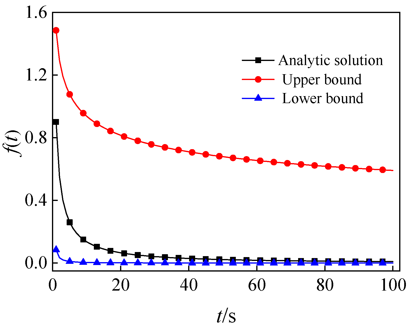
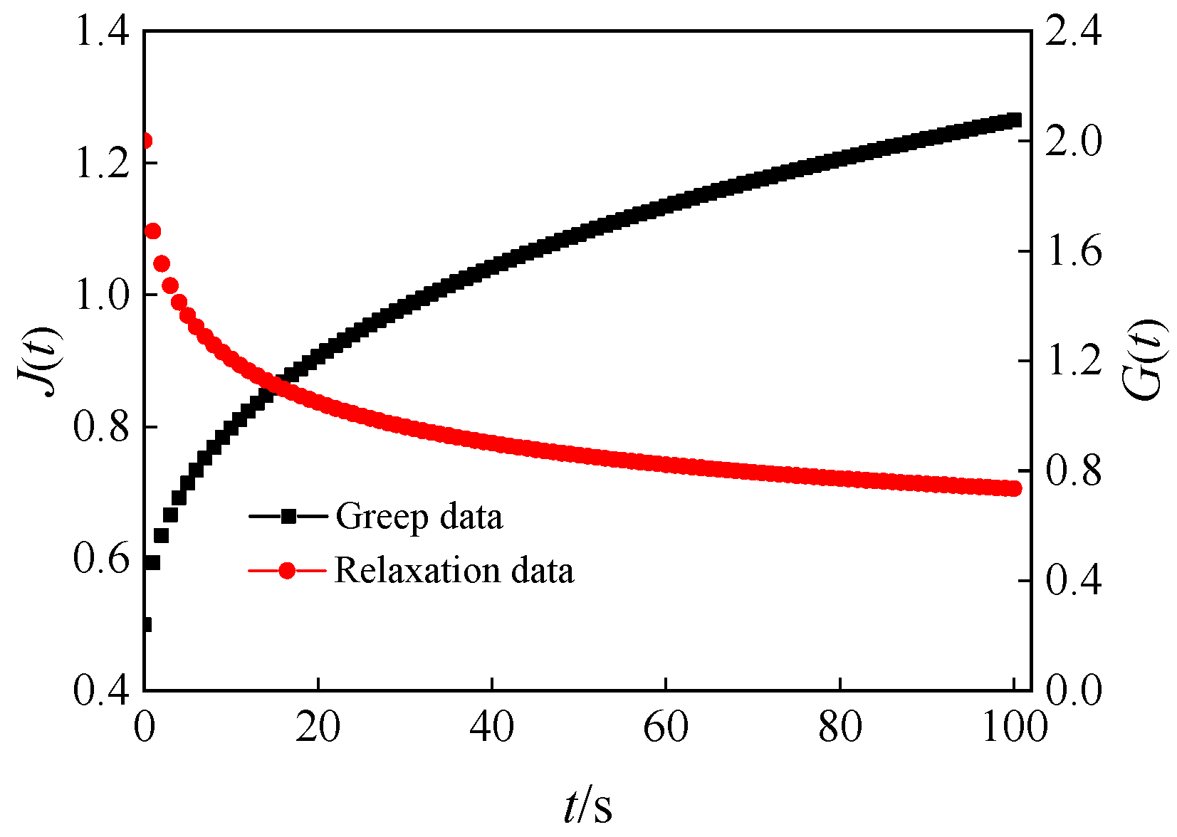
The integer-order three-parameter solid model was improved to a distributed order three-parameter solid model by introducing the distributed order damper. The creep compliance and relaxation modulus equations were obtained in the time domain by the Laplace transforms. After analysing the time-domain expressions of the distributed order operators, the operators’ upper and lower boundaries could be obtained. The theoretical results could reflect the creep properties and relaxation characteristics of the distributed order three-parameter solid model. This indicated that the model could reflect the viscoelastic properties of materials.

III.

Based on the single distributed order damage damper, the distributed order damage damper model was established by connecting the elements in series. Its corresponding constitutive equations and creep equations were established. The asymptotic properties of its two types of operators were analysed. Moreover, calculation examples were given to verify the creep properties of the model. The results showed that the established model could reflect the creep properties of the rock materials at the accelerated deformation stage. Moreover, as λ increased, the creep properties became more significant.

IV.

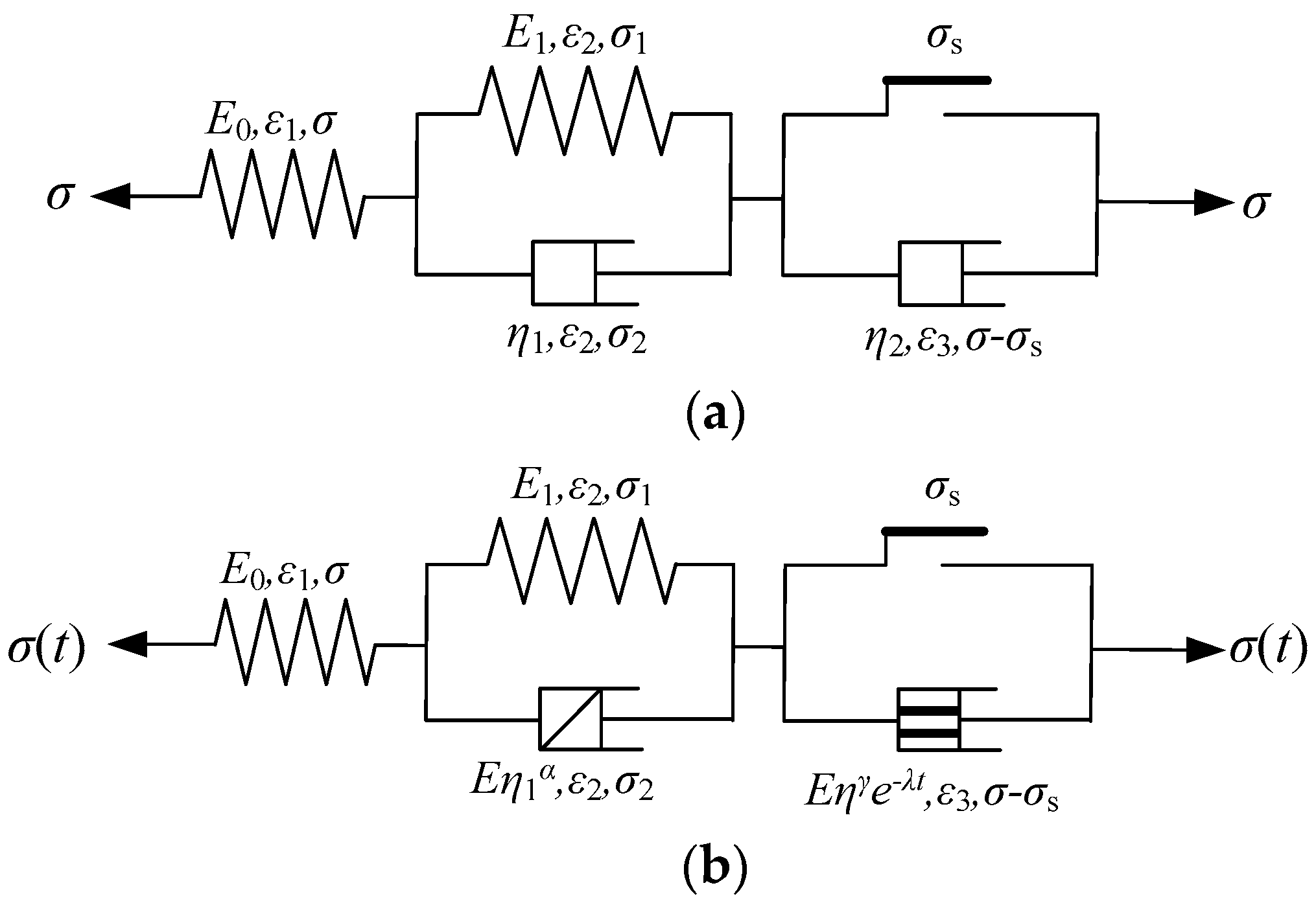
Based on the integer-order Nishihara model, the distributed order damage Nishihara model was established by introducing the fractional order damper and the distributed order damage damper. The creep properties equations were obtained. The specific calculation examples indicated that with proper damage parameters, the curves of the creep properties could better show the creep properties of the rock mass at the stages of instantaneous deformation, deceleration deformation, and acceleration deformation.

References

1. Zhao, C.; Yu, H.; Lin, Z.; Zhao, Y. Dynamic model and behaviour of viscoelastic beam based on the absolute nodal coordinate formulation. Proc. Inst. Mech. Eng. Part K J. Multi-Body Dyn. 2014, 229, 84–96. [Google Scholar] [CrossRef]
2. Rubin, M.B.; Nadler, B. An Eulerian formulation for large deformations of anisotropic elastic and viscoelastic solids and viscous fluids. Contin. Mech. Thermodyn. 2016, 28, 515–522. [Google Scholar] [CrossRef]
3. Lu, S.; Chung, D.D.L. Viscoelastic Behavior of Silica Particle Compacts under Dynamic Compression. J. Mater. Civ. Eng. 2014, 26, 551–553. [Google Scholar] [CrossRef]
4. Lang, L.; Song, K.-I.; Zhai, Y.; Lao, D.; Lee, H.-L. Stress Wave Propagation in Viscoelastic-Plastic Rock-Like Materials. Materials 2016, 9, 377. [Google Scholar] [CrossRef] [Green Version]
5. Zhang, J.; Green, H.W. Experimental Investigation of Eclogite Rheology and Its Fabrics at High Temperature and Pressure. J. Metamorph. Geol. 2007, 25, 97–115. [Google Scholar] [CrossRef]
6. Xie, S.; Pan, H.; Zeng, J.; Wang, E.; Chen, D.; Zhang, T.; Peng, X.; Yang, J.; Chen, F.; Qiao, S. A case study on control technology of surrounding rock of a large section chamber under a 1200-m deep goaf in Xingdong coal mine, China. Eng. Fail. Anal. 2019, 104, 112–125. [Google Scholar] [CrossRef]
7. Li, L. Studies of mineral properties at mantle condition using Deformation multi-anvil apparatus. Prog. Nat. Sci. 2009, 19, 1467–1475. [Google Scholar] [CrossRef]
8. Tian, X.; Xiao, H.; Li, Z.; Su, H.; Ouyang, Q.; Luo, S.; Yu, X. A Fractional Order Creep Damage Model for Microbially Improved Expansive Soils. Front. Earth Sci. 2022, 10, 942844. [Google Scholar] [CrossRef]
9. Aydan, Ö; Ito, T.; Özbay, U.; Kwasniewski, M.; Shariar, K.; Okuno, T.; Özgenoğlu, A.; Malan, D.F.; Okada, T. ISRM Suggested Methods for Determining the Creep Characteristics of Rock. Rock Mech. Rock Eng. 2014, 47, 275–290. [Google Scholar] [CrossRef] [Green Version]
10. Hou, R.; Zhang, K.; Tao, J.; Xue, X.; Chen, Y. A Nonlinear Creep Damage Coupled Model for Rock Considering the Effect of Initial Damage. Rock Mech. Rock Eng. 2019, 52, 1275–1285. [Google Scholar] [CrossRef]
11. Lyu, C.; Liu, J.; Ren, Y.; Liang, C.; Liao, Y. Study on very long-term creep tests and nonlinear creep-damage constitutive model of salt rock. Int. J. Rock Mech. Min. Sci. 2021, 146, 104873. [Google Scholar] [CrossRef]
12. Gao, Y.; Yin, D. A full-stage creep model for rocks based on the variable-order fractional calculus. Appl. Math. Model. 2021, 95, 435–446. [Google Scholar] [CrossRef]
13. Liu, H.Z.; Xie, H.Q.; He, J.D.; Xiao, M.L.; Zhuo, L. Nonlinear creep damage constitutive model for soft rocks. Mech. Time-Depend. Mater. 2017, 21, 73–96. [Google Scholar] [CrossRef]
14. Ma, L.; Wang, M.; Zhang, N.; Fan, P.; Li, J. A Variable-Parameter Creep Damage Model Incorporating the Effects of Loading Frequency for Rock Salt and Its Application in a Bedded Storage Cavern. Rock Mech. Rock Eng. 2017, 50, 2495–2509. [Google Scholar] [CrossRef]
15. Zhou, H.; Wang, C.; Han, B.; Duan, Z. A creep constitutive model for salt rock based on fractional derivatives. Int. J. Rock Mech. Min. Sci. 2011, 48, 116–121. [Google Scholar] [CrossRef]
16. Chen, J.; Jiang, Q.; Hu, Y.; Qin, W.; Li, S.; Xiong, J. Time-dependent performance of damaged marble and corresponding fractional order creep constitutive model. Arab. J. Geosci. 2020, 13, 1150. [Google Scholar] [CrossRef]
17. Wu, F.; Liu, J.F.; Wang, J. An improved Maxwell creep model for rock based on variable-order fractional derivatives. Environ. Earth Sci. 2015, 73, 6965–6971. [Google Scholar] [CrossRef]
18. Li, J.; Zhang, J.; Yang, X.; Zhang, A.; Yu, M. Monte Carlo simulations of deformation behaviour of unbound granular materials based on a real aggregate library. Int. J. Pavement Eng. 2023, 24, 2165650. [Google Scholar] [CrossRef]
19. Han, C.; Liu, X.; Li, D.; Shao, Y. Constitutive modeling of rock materials based on variable-order fractional theory. Mech. Time-Depend. Mater. 2021, 26, 485–498. [Google Scholar] [CrossRef]
20. Kawada, Y.; Yajima, T.; Nagahama, H. Fractional-order derivative and time-dependent viscoelastic behaviour of rocks and minerals. Acta Geophys. 2013, 61, 1690–1702. [Google Scholar] [CrossRef]
21. Sheikhani, P.P.A.H.R.; Najafi, H.S.; Ziabari, A.A. Numerical solution of fractional Mathieu equations by using block-pulse wavelets. J. Ocean. Eng. Sci. 2019, 4, 299–307. [Google Scholar] [CrossRef]
22. Ibrahim, R.W.; Meshram, C.; Hadid, S.B.; Momani, S. Analytic solutions of the generalized water wave dynamical equations based on time-space symmetric differential operator. J. Ocean Eng. Sci. 2020, 5, 186–195. [Google Scholar] [CrossRef]
23. Lorenzo, C.F.; Hartley, T.T. Variable Order and Distributed Order Fractional Operators. Nonlinear Dyn. 2002, 29, 57–98. [Google Scholar] [CrossRef]
24. Bansal, R.K. Approximation of surface–groundwater interaction mediated by vertical streambank in sloping terrains. J. Ocean Eng. Sci. 2017, 2, 18–27. [Google Scholar] [CrossRef] [Green Version]
25. Caputo, M. Linear Models of Dissipation whose Q is almost Frequency Independent—II. Geophys. J. Int. 1967, 13, 529–539. [Google Scholar] [CrossRef]
26. Bagley, R.L.; Torvik, P.J. On the existence of the order domain and the solution of distributed order equations. II. Int. J. Appl. Math. 2000, 2, 965–987. [Google Scholar]
27. Atanackovic, T.M.; Budincevic, M.; Pilipovic, S. On a fractional distributed-order oscillator. J. Phys. A Math. Gen. 2005, 38, 6703–6713. [Google Scholar] [CrossRef]
28. Atanackovic, T.M.; Pilipovic, S.; Zorica, D. Time distributed-order diffusion-wave equation. I. Volterra-type equation. Proc. R. Soc. A Math. Phys. Eng. Sci. 2009, 465, 1869–1891. [Google Scholar] [CrossRef]
29. Gerasimov, A.N. A generalization of linear laws of deformation and its application to problems of internal friction. Akad. Nauk SSSR. Prikl. Mat. Meh. 1948, 12, 251–260. [Google Scholar]
30. Atanackovic, T.M.; Pilipovic, S.; Zorica, D. Time distributed-order diffusion-wave equation. II. Applications of Laplace and Fourier transformations. Proc. R. Soc. A Math. Phys. Eng. Sci. 2009, 465, 1893–1917. [Google Scholar] [CrossRef]
31. Yuttanan, B.; Razzaghi, M.; Vo, T.N. A numerical method based on fractional-order generalized Taylor wavelets for solving distributed-order fractional partial differential equations. Appl. Numer. Math. 2020, 160, 349–367. [Google Scholar] [CrossRef]
32. Atanackovic, T.M.; Pilipovic, S.; Zorica, D. Existence and calculation of the solution to the time distributed order diffusion equation. Phys. Scr. 2009, 014012. [Google Scholar] [CrossRef]
33. Mainardi, F.; Pagnini, G. The role of the Fox–Wright functions in fractional sub-diffusion of distributed order. J. Comput. Appl. Math. 2007, 207, 245–257. [Google Scholar] [CrossRef] [Green Version]
34. Pourbabaee, M.; Saadatmandi, A. The construction of a new operational matrix of the distributed-order fractional derivative using Chebyshev polynomials and its applications. Int. J. Comput. Math. 2021, 98, 2310–2329. [Google Scholar] [CrossRef]
35. Chen, W.; Sun, H.; Zhang, X.; Korošak, D. Anomalous diffusion modeling by fractal and fractional derivatives. Comput. Math. Appl. 2010, 59, 1754–1758. [Google Scholar] [CrossRef] [Green Version]
36. Bu, W.; Xiao, A.; Zeng, W. Finite Difference/Finite Element Methods for Distributed-Order Time Fractional Diffusion Equations. J. Sci. Comput. 2017, 72, 422–441. [Google Scholar] [CrossRef]
37. Veeresha, P.; Prakasha, D.; Magesh, N.; Christopher, A.J.; Sarwe, D.U. Solution for fractional potential KdV and Benjamin equations using the novel technique. J. Ocean Eng. Sci. 2021, 6, 265–275. [Google Scholar] [CrossRef]
38. Hartley, T.T.; Lorenzo, C.F. Fractional-order system identification based on continuous order-distributions. Signal Process. 2003, 83, 2287–2300. [Google Scholar] [CrossRef]
39. Rahimkhani, P.; Ordokhani, Y. Approximate solution of nonlinear fractional integro-differential equations using fractional alternative Legendre functions. J. Comput. Appl. Math. 2019, 365, 112365. [Google Scholar] [CrossRef]
40. Liu, W.; Röckner, M.; da Silva, J.L. Strong dissipativity of generalized time-fractional derivatives and quasi-linear (stochastic) partial differential equations. J. Funct. Anal. 2021, 281, 109135. [Google Scholar] [CrossRef]
41. Xu, M.; Tan, W. Intermediate processes and critical phenomena: Theory, method and progress of fractional operators and their applications to modern mechanics. Sci. China Phys. Mech. Astron. 2006, 49, 257–272. [Google Scholar] [CrossRef]
42. Kochubei, A.N. Distributed order calculus and equations of ultraslow diffusion. J. Math. Anal. Appl. 2007, 340, 252–281. [Google Scholar] [CrossRef] [Green Version]
43. Luchko, Y. Initial-boundary-value problems for the generalized multi-term time-fractional diffusion equation. J. Math. Anal. Appl. 2011, 374, 538–548. [Google Scholar] [CrossRef] [Green Version]
44. Gao, G.-H.; Sun, Z.-Z. Two alternating direction implicit difference schemes with the extrapolation method for the two-dimensional distributed-order differential equations. Comput. Math. Appl. 2015, 69, 926–948. [Google Scholar] [CrossRef]
45. Mainardi, F.; Mura, A.; Gorenflo, R.; Stojanović, M. The Two Forms of Fractional Relaxation of Distributed Order. J. Vib. Control 2007, 13, 1249–1268. [Google Scholar] [CrossRef] [Green Version]
46. Cao, L.; Pu, H.; Li, Y.; Li, M. Time domain analysis of the weighted distributed order rheological model. Mech. Time-Depend. Mater. 2016, 20, 601–619. [Google Scholar] [CrossRef]
47. Cao, L.; Li, Y.; Tian, G.; Liu, B.; Chen, Y. Time domain analysis of the fractional order weighted distributed parameter Maxwell model. Comput. Math. Appl. 2013, 66, 813–823. [Google Scholar] [CrossRef]
48. Hou, R.; Xu, L.; Zhang, D.; Shi, Y.; Shi, L. Experimental Investigations on Creep Behavior of Coal under Combined Compression and Shear Loading. Geofluids 2021, 2021, 9965228. [Google Scholar] [CrossRef]
49. Li, G.; Wang, Y.; Wang, D.; Yang, X.; Yang, S.; Zhang, S.; Li, C.; Teng, R. An unsteady creep model for a rock under different moisture contents. Mech. Time-Depend. Mater. 2022, 1–15. [Google Scholar] [CrossRef]
Figure 1. Model of the distributed order damper. (a) Standard form of the distributed order damper, (b) Simplified form.
Applsci 13 04404 g001
Figure 2. The three-parameter solid model. (a) The integer-order three-parameter solid model, (b) The distributed order three-parameter solid model.
Applsci 13 04404 g002
Figure 3. Contour integral of the inverse Laplace transform.
Applsci 13 04404 g003
Figure 4. Path of Hankel integral.
Applsci 13 04404 g004
Figure 5. Characteristics of f(t).
Applsci 13 04404 g005
Figure 6. Response characteristics of the rheological properties of the distributed order rheological model.
Applsci 13 04404 g006
Figure 7. The distributed order damage damper. (a) Standard form of the distributed order damage damper, (b) The simplified form.
Applsci 13 04404 g007
Figure 8. Curves of the creep properties of the distributed order damper with various damage parameters.
Applsci 13 04404 g008
Figure 9. The distributed order damage creep model of the rock mass. (a) The integer-order Nishihara model, (b) The distributed order damage Nishihara model.
Applsci 13 04404 g009
Figure 10. Curves of the creep properties of the rock mass under various damage.
Applsci 13 04404 g010
Disclaimer/Publisher’s Note: The statements, opinions and data contained in all publications are solely those of the individual author(s) and contributor(s) and not of MDPI and/or the editor(s). MDPI and/or the editor(s) disclaim responsibility for any injury to people or property resulting from any ideas, methods, instructions or products referred to in the content.