Article

Hybrid EMD-RF Model for Predicting Annual Rainfall in Kerala, India

by
Asha Jayasree
1,*,
Santhosh Kumar Sasidharan
2,
Rishidas Sivadas
2 and
Jayan A. Ramakrishnan
1
1
Department of Electronics and Communication Engineering, Government Engineering College Thrissur, APJ Abdul Kalam Technological University, Thrissur 680009, India
2
Department of Electronics and Communication Engineering, Government Engineering College Idukki, APJ Abdul Kalam Technological University, Painavu 685603, India
*
Author to whom correspondence should be addressed.
Appl. Sci. 2023, 13(7), 4572; https://doi.org/10.3390/app13074572
Submission received: 4 March 2023 / Revised: 28 March 2023 / Accepted: 30 March 2023 / Published: 4 April 2023

Abstract

:
Rainfall forecasting is critical for the economy, but it has proven difficult due to the uncertainties, complexities, and interdependencies that exist in climatic systems. An efficient rainfall forecasting model will be beneficial in implementing suitable measures against natural disasters such as floods and landslides. In this paper, a novel hybrid model of empirical mode decomposition (EMD) and random forest (RF) was developed to enhance the accuracy of annual rainfall prediction. The EMD technique was utilized to decompose the rainfall signal into six intrinsic mode functions (IMFs) to extract underlying patterns, while the RF algorithm was employed to make predictions based on the IMFs. The hybrid RF–IMF model was trained and tested using a dataset of annual rainfall in Kerala from 1871 to 2020, and its performance was compared to traditional models such as RF regression and the autoregressive moving average (ARMA) model. Mean absolute error (MAE), mean absolute percentage error (MAPE), mean squared error (MSE), root mean squared error (RMSE), and coefficient of determination or R-squared (R2) were used to compare the performances of these three models. Model evaluation metrics show that the RF–IMF model outperformed both the RF model and ARMA model.

1. Introduction

The Indian economy is mostly reliant on agriculture; hence, annual rainfall is quite important. The summer monsoon, which lasts from June to September, is responsible for the majority of the rainfall. Any variations in rainfall have a significant impact on the agriculture sector and, as a result, the economy of the country. The annual rainfall of Kerala state in India is forecasted in this study. Kerala receives an average annual rainfall of over 3000 mm, which is quite heavy when compared to the Indian average of roughly 1000 mm. The Southwest monsoon is responsible for 70% of Kerala’s annual rainfall. Kerala is known as the “Monsoon Gateway” since it is the first state in India to receive the rains. Kerala was historically known for its temperate and pleasant climate, owing to its abundant annual rainfall and proximity to the Western Ghats and the Indian Ocean. However, the state has recently felt the brunt of uncertain climate change. Extreme rainfall, floods, landslides, heat waves, sunstrokes, and cyclones have all become increasingly regular in recent years. One of the greatest floods in the state’s history struck in 2018, killing hundreds of people and affecting roughly one-sixth of the state’s population. Floods and landslides struck Kerala’s northern districts again in 2019, causing countless tragedies. Considering this scenario, having a better yearly rainfall prediction model is critical. Many attempts have been made in India to predict rainfall at the regional and national levels. Probabilistic and deterministic methods such as ARMA-based methods were used to predict rainfall using the hydrological datasets. However, these approaches have limitations such as nonlinearity and non-stationarity.
The primary objective of this work was to predict the annual rainfall of Kerala based on the rainfall time series data from 1871 to 2020. The data for this period are available on the websites of the Indian Institute of Tropical Meteorology and the Indian Meteorological Department. Annual rainfall data are very nonlinear and non-stationary in time series. This makes statistical methods to make a forecast challenging. This work proposes empirical mode decomposition based on random forest regression to predict the annual rainfall. The suggested model was compared to the ARMA and RF regression models to assess its performance. Mean absolute error (MAE), mean absolute percentage error (MAPE), mean squared error (MSE), root mean squared error (RMSE), and coefficient of determination or R-squared (R2) values were used to evaluate the forecasting ability of these three models. Several studies have been conducted to investigate long-term as well as short-term rainfall prediction using conventional statistical and machine learning methods. Support vector regression (SVM) and multilayer perception (MLP) were used for the annual rainfall prediction of Odisha, India. The SVM model exhibited better performance than MLP with an R-value of 0.9 [1]. Artificial neural networks-multilayer perception was used to forecast 15 years of rainfall across India using rainfall data from 1901 to 2015. The work investigated the variability and predicted the trend of rainfall in various regions of India [2]. Hybrid models were used for monthly rainfall prediction in Vietnam, where the time-series data were decomposed using two pre-processing methods—seasonal decompositions and discrete wavelet transform. This pre-processed data were fed to artificial neural networks (ANN) and seasonal ANN prediction (SANN) models. The work found out that Meyer wavelet–SANN model gave the best prediction with R-value, MAE, and RMSE as 0.997, 9.32 and 12 mm, respectively [3]. The inter-annual variability of India’s Southwest monsoon rainfall was investigated using empirical mode decomposition and forecasting modeling was carried out using ANN. All India rainfall for the year 2004 and its standard deviation were forecasted as 80.34 and 3.3 cm, respectively [4]. A random forest regression was trained to learn a quantitative precipitation estimation model directly from a four-year database [5]. It was observed that the random forest algorithm significantly reduced the error and bias of predicted precipitation intensities. Four different machine learning algorithms including decision forest regression were used to develop rainfall forecasting models [6]. Decision tree and stochastic forest algorithm were used to predict summer precipitation in Chongqing, from 2011 to 2018 [7]. A seasonal ARIMA model was applied to predict the mean temperature and precipitation in the Bhagirathi river basin in Uttarakhand, India [8]. The annual rainfall in Hyderabad was predicted using ANN and autoregressive integrated moving average (ARIMA) approaches [9]. ARIMA was used to predict annual rainfall and maximum temperature over the Tordzie watershed in Ghana [10].
The abovementioned techniques of rainfall prediction could not account for the non-stationarity and non-linearity of rainfall data. Meanwhile, empirical mode decomposition was used as an effective tool in handling non-stationary data and was employed in many fields. Some of them are: EMD analyses of climate changes were performed with reference to rainfall data [11]. Their study suggested that EMD is an effective tool in isolating physical processes of various time scales. Ensemble EMD was used to isolate the rainfall and temperature data in different time scales and used to identify the variability [12]. Hybrid EMD models were employed in various fields for prediction. An energy time series forecasting based on empirical mode decomposition and fuzzy radial basis function and the Autoregressive model was developed [13]. EMD and support vector regression were combined to forecast financial time series [14]. Their work showed that EMD has improved forecasting, by capturing the local fluctuations of time series.
In the literature, Li and Wang, 2008, Zheng et al., 2013, Tatinati and Kalyana, 2013, Ren, Suganthan, and Srikanth, 2016, and Zhang et al., 2016 [15,16,17,18,19] had utilized hybrid EMD models for making predictions using nonlinear and non-stationary time series wind speed data. All these works have utilized EMD as an effective tool in decomposing non-stationary and non-linear data into IMFs and trend signals and a suitable forecasting model is used to predict future IMFs. These hybrid models are found to be effective in improving forecasting accuracy. This paper used EMD to decompose the rainfall data and random forest regression is used to make the annual rainfall prediction. This novel combination of EMD and RF provides improved accuracy and proves to be an efficient algorithm for reducing errors in prediction.

2. Methodologies and Dataset

The efficacy of the proposed methodology is understood by comparing the performance of the proposed RF–IMF model with the ARMA and RF models. The principle of each methodology is explained below.

2.1. ARMA

The general auto-regressive moving average (ARMA) model was first described by Peter Whittle, in 1951, in his thesis titled “Hypothesis testing in time series analysis”. Box and Jenkins [20] popularized the ARMA model and later introduced the auto-regressive integrated moving average (ARIMA) model. ARIMA model transforms a non-stationary series into a stationary series by differencing. ARIMA model has three components:
(i)
AR part indicates the autocorrelation between present and past values.
(ii)
MA part indicating the autocorrelation between present and past values of the error term.
(iii)
Integrated part (I), denoting the level of differencing required to make the time series stationary.
ARIMA p , q , d is expressed in terms of lag polynomials as:
Φ M 1 M d y t = θ M ε t
1 i = 1 p Φ i M i 1 M d y t = 1 + j = 1 q Φ j M j ε t
where M is the backshift operator; Φ M is the AR operator and p is the order of AR; θ M is the MA operator of error term ε t and q is its order; d is the differencing level.
If the value of d is 0, then the model reduces to an ARMA p , q model.
Auto ARIMA method was used to generate the optimized values of p , q and d that were best suited for prediction. The optimum model was identified based on the values of the Akaike Information Criterion (AIC) and Bayesian Information Criterion (BIC) [21].
A I C = 2 N l o g l i k e l i h o o d + 2 m N
B I C = 2 l o g l i k e l i h o o d + ln N m
The stationarity of the series was tested using the Augmented Dickey–Fuller (ADF) method [22]. The AIC and BIC values were used by the Auto ARIMA model to determine the best p , q and d values for forecasting. The Auto ARIMA capability was provided by the Python module ‘pmdarima’. Auto ARIMA starts by running differencing tests, with the Augmented Dickey–Fuller (ADF) test being the most popular. The ADF test examines if a series has a unit root and, as a result, whether it is stationary or not. ADF test uses an autoregressive model and optimizes one information criterion. The criterion used in this work was AIC. The null hypothesis was that the time series was not stationary and the alternate hypothesis was that the time series was stationary. The result of the ADF test was interpreted using the p-value. If the p-value is less than the threshold value of 5%, then the null hypothesis is rejected otherwise alternative hypothesis is rejected. Algorithm 1 elaborates the algorithm for Auto ARIMA.
Algorithm 1: Auto ARIMA prediction model
The algorithm for prediction using Auto ARIMA is given below:
  • Load the time series data.
  • Use Auto ARIMA to find the optimum ARIMA model.
    (i)
    Augmented Dickey–Fuller (ADF) test was used to determine the stationarity, which tests the null hypothesis that the series is non-stationary.
    (ii)
    AIC and BIC were used to fix the values of ‘ p ’ and ‘ q ’.
  • Split the data into training and testing datasets.
  • Fit the identified model on the training dataset.
  • Predicted the value of the testing dataset.
  • Evaluated the performance metrics.

2.2. Random Forest Regression

Random forest is a supervised learning algorithm consisting of an ensemble of decision trees [23]. It is used for both classification and regression problems. The RF algorithm is trained through both bootstrap aggregating and bagging. An RF algorithm is built using decision trees. A decision tree has three parts-root nodes, decision nodes, and leaf nodes. The root node comprises the whole predictor space. The trees used in RF are based on binary recursion partitioning trees. Leaf nodes are nodes that have not been split and form the ultimate decision. The dataset was first split into training and testing datasets. A sliding window approach was used for annual rainfall prediction, with the window size remaining fixed. The main hyperparameter was the number of estimators or the number of trees in the forest and the number of random states. Scikit-Learn’s Randomized Search CV method was used to define a set of optimum hyperparameter values Algorithm 2.
Algorithm 2: Random Forest for Regression
  • For n = 1 to N:
    (i)
    Draw a bootstrap sample of size s’ from training data.
    (ii)
    Grow an RF tree Rn to the bootstrapped data, by repeating the below steps for each leaf node of the tree, until the minimum node size is reached.
       Steps
    (a)
    Select ‘k’ variables randomly.
    (b)
    Choose the best split-point among ‘k’ variables out of ‘p’ variables.
    (c)
    Split the node into two nodes.
  • Output the ensemble of trees { R n }.The predictions from each tree at a point ‘x’ are averaged for regression.

2.3. RF–IMF

2.3.1. Empirical Mode Decomposition

Huang first proposed EMD in 1998. Non-stationary and nonlinear signals are decomposed into a finite number of components using EMD. For the original signal, these components constitute a nearly orthogonal basis. The decomposed signals are called the intrinsic mode functions (IMFs) [24]. IMFs have characteristic time scales of oscillations defined by the local maxima and local minima of the data. IMFs are derived from the data themselves without using any functional form. IMFs are locally stationary, oscillating around zero. Additionally, each IMF has a characteristic oscillation period. In short, with EMD, the complexity of the data is reduced by separating trends and oscillations at different scales.
EMD is a useful technique for breaking down the nonlinear and non-stationary time series into intrinsic mode functions and a monotonic function known as trend or residue. The signal may be reconstructed by combining the parts together because this decomposition is additive. EMD’s components or IMFs can be utilized as input to any regression or classification model. EMD and random forest regression were coupled in this work to forecast annual rainfall. An IMF has:
(i)
Only one extreme between zero crossings;
(ii)
Mean value of IMF is zero;
(iii)
The number of extremes are either equal or differs by a maximum of one.
The processsfor obtaining IMFs from the time-series signal is as follows:
Let   y t be the input time-series signal
1.
Initialization
i = 1 Y t = y t
2.
Locate all local maximum and local minimum values of the input signal Y t .
Find the upper envelope y max t by connecting all the local maxima by a spline curve; do the same with all the local minima and find y min t .
3.
Calculate the local mean
m i 1 t = y min t + y max t 2
4.
Find the difference between the input signal and the mean
h i t = Y t m i 1 t
5.
If the stopping criteria are satisfied by h i t then
IMF i = h i t   else   Y t = h i t
and start again from step 1
6.
Y t = Y t IMF i ,   i = i + 1
7.
The sifting process is stopped if the residual signal Y t becomes a monotonic or residue function ( r t ). The original signal can be written as the summation of all IMFs and residue function:
Y t = i = 1 n h i t + r t
where n denotes the number of IMFs and r(t) is the trend signal. Figure 1 shows the flowchart for empirical mode decomposition.

2.3.2. RF–IMF

The original annual rainfall time series is broken down into five intrinsic mode functions and a residual series. Then, these subseries are modeled using the random forest regression model so that the future values can be predicted. The predicted values of all the IMFs are aggregated to forecast the annual rainfall. The training dataset comprises annual rainfall values from 1871 to 2000, whereas the testing dataset is selected to be from 2001 to 2020. Empirical mode decomposition was implemented using the PyEMD package in Python. The implementation of sifting algorithm was carried out using the emd.sift module in the package. The algorithm for RF–IMF forecasting model is shown in Algorithm 3.
Algorithm 3: RF–IMF prediction model
The algorithm for prediction using RFIMF is given below:
1.
Load the annual rainfall data series Y where, Y= {x(1), x(2),... x(n)}
2.
Decompose Y into five IMFs and one residue series.
3.
Pearson cross-correlation matrix is obtained among the original time series, IMFs, and the residue. A strong correlation exists between the original time series and IMF1. Similar correlations exist between adjacent IMFs.
4.
The future IMFs are predicted using random forest regression.
Each IMF is forecasted as per the following RF models:
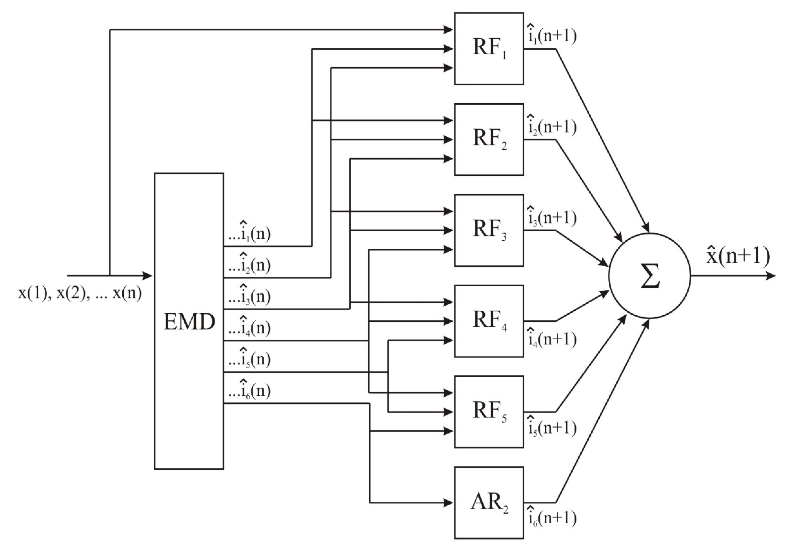
i ^ i n + 1 is the ith predicted IMF, n + 1 th IMFs are predicted using the n th adjacent IMFs. Since i ^ 6 n + 1 is the trend signal, it is predicted using the auto regression of i ^ 6 n . The expressions for predicted IMFs are:
i ^ i n + 1 = R F Y , i ^ 1 n , i ^ 2 n ,
i 2 n + 1 = R F i ^ 1 n , i ^ 2 n , i ^ 3 n ,
i ^ 3 n + 1 = R F i ^ 2 n , i ^ 3 n , i ^ 4 n
i ^ 4 n + 1 = R F i ^ 3 n , i ^ 4 n , i ^ 5 n
i ^ 5 n + 1 = R F i ^ 4 n , i ^ 5 n , i ^ 6 n ,
i ^ 6 n + 1 = A R i ^ 6 n
  x ^ n + 1 = i = 1 6 i ^ i n + 1 .
Figure 2 displays the RF–IMF forecasting model, which predicts each IMF using RF and combines them to obtain the forecasted annual rainfall.

2.4. Dataset

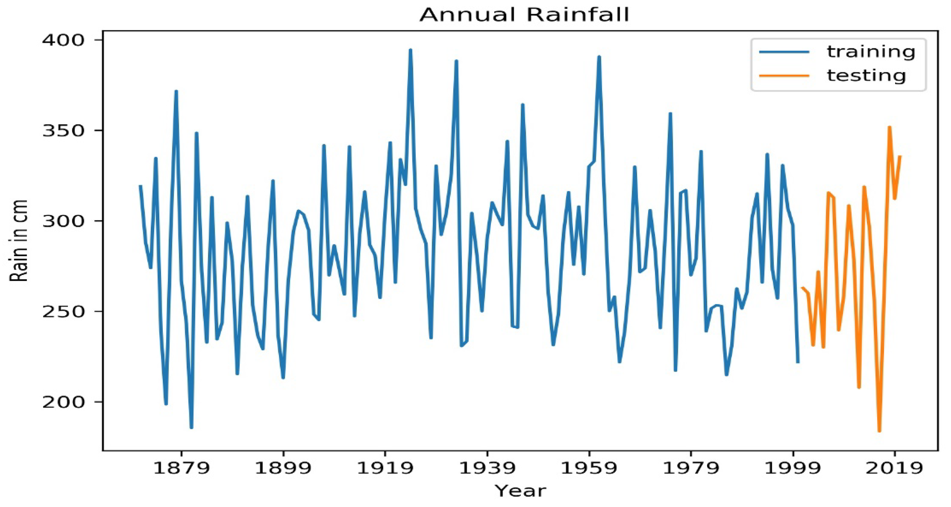
The Indian Institute of Tropical Meteorology (IITM) website (https://www.tropmet.res.in/data/data-archival/rain/iitm-regionrf.txt, accessed on 20 May 2021) [25] has annual rainfall data for the Kerala state from 1871 to 2016. This rainfall data are based on a fixed network of 10 rain gauge stations located throughout Kerala. One rain gauge station is placed for every 3886.4 square kilometers. The yearly rainfall statistics report of the Indian Meteorological Department provided rain data from 2017 to 2020. Thus, the total data acquired span a period of 150 years. The entire data from 1871 to 2020 were partitioned into training and testing datasets. In this work, the training dataset ranges from 1871 to 2000, whereas the testing dataset was rainfall data from 2001 to 2020, which formed approximately 12% of the total dataset.
The model was prepared on the training dataset while the forecasting was made for the test dataset. Using the trained model, a one-step forecast of annual rainfall was created based on the ‘L’ previous data. The actual observation from the test set was then added to the training dataset and the model was refitted. This process was repeated for the entire test dataset. This model is called the walk forward testing. Since the training window was a sliding one, this model is also called a rolling forecast [26]. Figure 3 depicts the rolling forecast model that was used in random forest-based prediction. Previous ‘L’ years rain data were used to predict the ‘L+1’th year rain and the actual rain of ‘L+1’ year was used to predict the rain for the subsequent year, and this was continued for the entire testing dataset.

2.5. Assessment Indicators for Predicting Performance

To evaluate and compare the forecasting capability of ARMA, RF and the proposed RF–IMF model the following evaluation metrics were applied. In the performance metrics explained below, x i   represents the actual value, x i ^ , its predicted value, x   ¯ is the mean value and N represents the number of testing datasets.
(i)
Mean absolute error (MAE): It represents the mean of the absolute difference between the actual and forecasted values.
M A E = 1 N i = 1 N x i x i ^
(ii)
Mean squared error (MSE): It is defined as the average of the squared difference between the actual and predicted values, or, in other words, it is the measurement of the variance.
M S E = 1 N i = 1 N x i x i ^ 2
(iii)
Root mean square error (RMSE): It is the square root of the MSE or it is the measurement of standard deviation.
R M S E = 1 N i = 1 N x i x i ^ 2 0.5
(iv)
Mean absolute percentage error (MAPE): It is the percentage equivalent of MAE. This can easily be interpreted and explained.
M A P E = 100 / N i = 1 N x i x i ^ x i
(v)
Coefficient of determination or R2: R-squared represents the proportion of variance in the dependent variable. It indicates how well a model fits the given dataset or it analyses how well a variable predicts another one. It lies between 0 and 1 and a larger value indicates a better fit between the predicted and actual value. R-squared value explains the strength of linear relationship between two variables. It can be used for evaluating trend analysis [27].
R 2 = 1 i = 1 N x i x i ^ 2 i = 1 N x i x i ¯ 2

3. Annual Rainfall Prediction

3.1. Auto ARIMA

The results of ADF test were as follows:
ADF statistics: −10.534
p-Value: 0
Critical values: 1%: −3.479, 5%: −2.883, 10%: −2.578
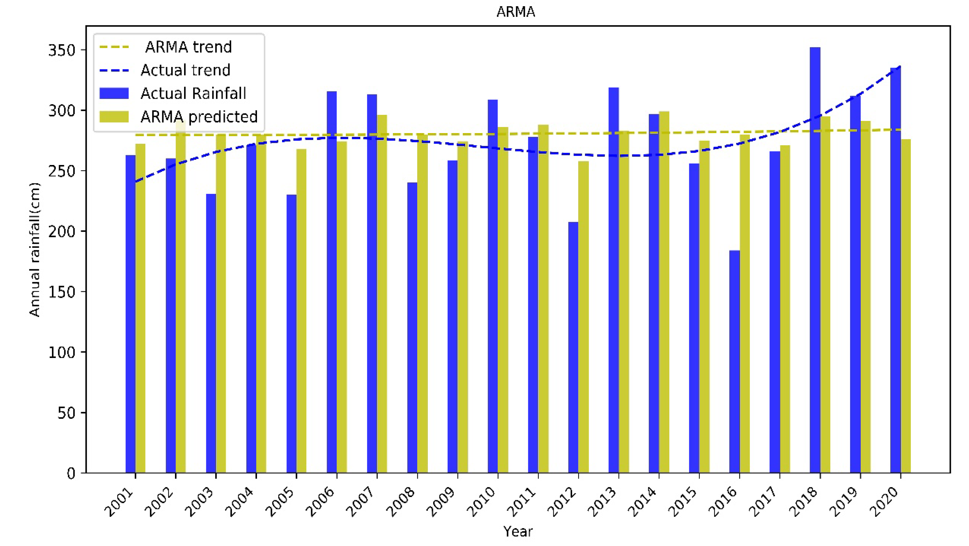
Figure 4 illustrates the total annual rainfall from 1871 to 2020, with training and testing data shown in different colors. The optimized ARIMA model’s accuracy could be checked by comparing the predicted values of annual rainfall with the observed rainfall. Figure 5 shows a bar chart of the predicted values versus actual annual rainfall between the years 2001 and 2020 for the ARMA model and their trend lines. The bar chart indicates that even though the ARMA model succeeded in predicting the rainfall, with minor errors, in some of the years, it failed in predicting the overall trend in rainfall. The trend lines indicate that the ARMA model fails in following the trend of actual rainfall.

3.2. Random Forest Regression Model

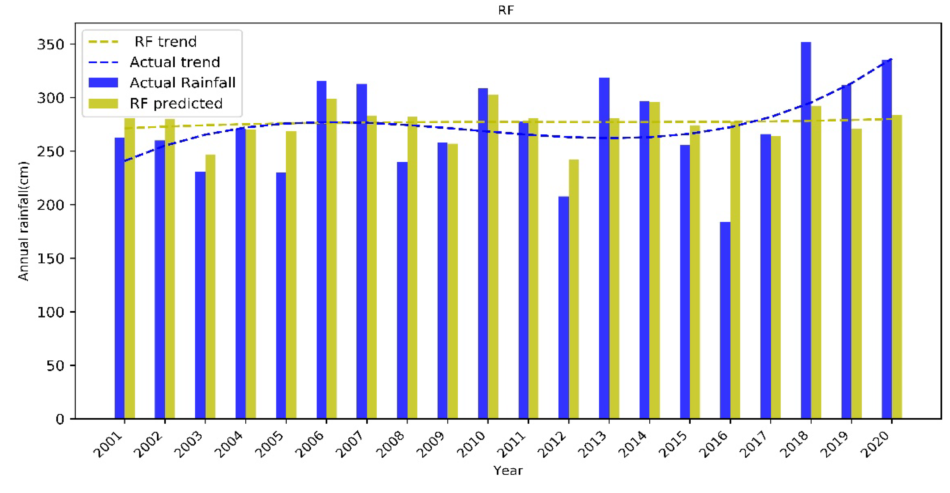
The number of estimators obtained using hyperparameter tuning was 150, the number of random states obtained was 10, the maximum depth was 110 and the size of the rolling window ‘L’ was 5. After fixing the hyperparameter values, the RF regression model was imported from Scikit-Learn and then the model was instantiated and fitted on the training data, with the size of the window fixed as 5. Then, the prediction was made on the testing dataset, which ranges between 2001 and 2020. The predicted rainfall was compared with the actual rainfall and the performance of the RF model was evaluated based on the metrics mentioned. Figure 6 shows the bar chart of the predicted values versus the actual rainfall for the RF model. The RF model shows an improved performance in predicting the annual rainfall value; however, the error for the years 2016, 2018 to 2020 still remains high.

3.3. RF–IMF Prediction Model

In this proposed model for annual rainfall prediction, as the first step, the original time series was decomposed into IMFs and the Pearson correlation coefficient(PCC) [28] was calculated among the different IMFs and the original time series. PCC is defined as the ratio between the covariance of two signals and the product of their standard deviations. The values of coefficients obtained are listed in Table 1.
PCC values show that adjacent IMF values are highly correlated; thus, the random forest model for predicting the future IMFs was modeled with adjacent IMFs as inputs. The flowchart (Figure 1) depicts the modeling of the RF–IMF forecasting model. Figure 7 depicts the intrinsic mode functions obtained via empirical mode decomposition of the original time series. Blue colour indicates testing dataset and pink colour is the predicted IMF’s. Here, IMF1 to IMF3 are the high-frequency components, IMF4 and IMF5 are the medium-frequency components and IMF6, the low-frequency trend signal.
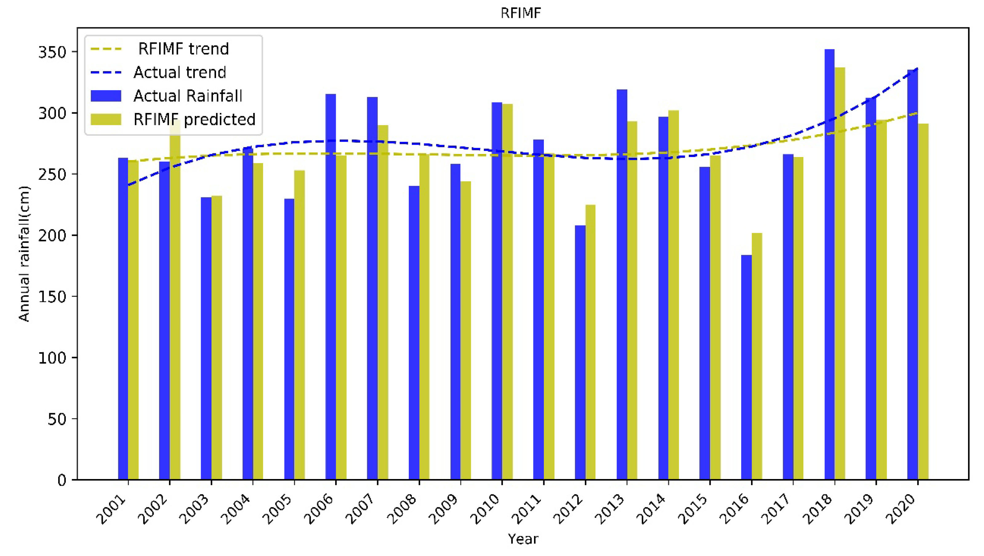
The IMFs from 1871 to 2000 came from the testing dataset, while the IMFs from 2001 to 2020 were their predicted values. The predicted IMFs from 2001 to 2020 were combined to obtain the corresponding year’s annual rainfall. Figure 8 shows the bar chart of the predicted values versus the actual rainfall for the RF–IMF model. The bar chart and trend lines clearly indicate that the error values have been reduced and succeeded in predicting the trend in annual rainfall.

4. Performance Evaluation and Discussion

To compare the predictive performance of the proposed RF–IMF model with ARMA and random forest models, the predicted values of the testing time period are compared. Table 2 compares the actual rainfall value with the predicted values of all three models from 2001 to 2020.
Both the ARMA and RF models failed in tracking the rapid variations in annual rainfall; however, the proposed RF–IMF model succeeded in predicting the extreme annual rainfall. This is clear from the predicted rainfall values for years 2018 to 2020. The year 2018 reported the highest rainfall ever in the history of Kerala, resulting in the largest flood the state has ever witnessed. The RF–IMF model predicted a value of 337cm, which is much closer to the actual value of 352cm. The comparison of these models based on the performance metrics such as MAE, MSE, RMSE, MAPE and R2 are presented in Table 3.
MAE, MSE, RMSE and MAPE were the error type measures of the deviation of predicted results from actual values. Lower values of these indicate better prediction, while a higher value of R2 is desirable. The higher the R2 value, the better the model is at predicting rainfall. The values in Table 3 indicate that the proposed RF–IMF model gives the highest accuracy as it has the lowest values for all the error metrics and highest value of R2. The R2 score of RF–IMF is 0.76, which is much higher than the other two models, indicating its power to follow the trend in annual rainfall pattern. Even though the proposed RF–IMF model outperforms the other two models, the extreme amount of rainfall seen in the recent years poses a challenge to our prediction model. Incorporating the various climatic indices such as ENSO (El Nino Southern Oscillation), IOD (Indian Ocean Dipole) and SST (sea surface temperature) will definitely improve the prediction accuracy.

5. Conclusions

This paper proposed a method for predicting the annual rainfall based on EMD and RF. Using EMD, the annual rainfall time series data were decomposed into five IMFs and a residue. Random forest regression predicted the future IMFs and residue for the testing time period. The forecasted IMFs and the residue were aggregated to obtain the final predicted value. In terms of the different performance metrics, RF–IMF model outperforms ARMA and RF models. The ARMA and RF models’ ability to predict the trend of next year’s rainfall is poorer when compared to that of the RF–IMF model and this is indicated by their R-squared values. Thus, the proposed RF–IMF model can be used as an efficient forecasting tool to predict the annual rainfall. The efficiency of the predictions may be further improved by considering the effects of ENSO, SST and IOD indices.

Author Contributions

Conceptualization, A.J. and S.K.S.; methodology, A.J. and S.K.S.; software, A.J. and S.K.S.; validation, A.J., S.K.S., R.S. and J.A.R.; formal analysis, A.J.; investigation, A.J.; resources, A.J. and S.K.S.; data curation, A.J. and S.K.S.; writing—original draft preparation, A.J.; writing—review and editing A.J., S.K.S. and J.A.R.; visualization, A.J. and S.K.S.; supervision, S.K.S., R.S. and J.A.R. All authors have read and agreed to the published version of the manuscript.

Funding

This research received no external funding.

Institutional Review Board Statement

Not appicable.

Informed Consent Statement

Not applicable.

Data Availability Statement

Rainfall data was collected from https://www.tropmet.res.in/data/data-archival/rain/iitm-regionrf.txt (accessed on 20 May 2021).

Conflicts of Interest

The authors declare no conflict of interest.

References

  1. Zhang, X.; Mohanty, S.N.; Parida, A.K.; Pani, S.K.; Dong, B.; Cheng, X. Annual and Non-Monsoon Rainfall Prediction Modelling Using SVR-MLP: An Empirical Study From Odisha. IEEE Access 2020, 8, 30223–30233. [Google Scholar] [CrossRef]
  2. Praveen, B.; Talukdar, S.; Mahato, S.; Mondal, J.; Sharma, P.; Islam, A.R.T.; Rahman, A. Analyzing trend and forecasting of rainfall changes in India using non-parametrical and machine learning approaches. Sci. Rep. 2020, 10, 10342. [Google Scholar] [CrossRef] [PubMed]
  3. Tran Anh, D.; Duc Dang, T.; Pham Van, S. Improved Rainfall Prediction Using Combined Pre-Processing Methods and Feed-Forward Neural Networks. J 2019, 2, 65–83. [Google Scholar] [CrossRef] [Green Version]
  4. Iyengar, R.N.; Raghu Kanth, S.T.G. Intrinsic mode functions and a strategy for forecasting Indian monsoon rainfall. Meteorol. Atmos. Phys. 2005, 90, 17–36. [Google Scholar] [CrossRef] [Green Version]
  5. Wolfensberger, D.; Gabella, M.; Boscacci, M.; Germann, U.; Berne, A. RainForest: A random forest algorithm for quantitative precipitation estimation over Switzerland. Atmos. Meas. Tech. 2021, 14, 3169–3193. [Google Scholar] [CrossRef]
  6. Ridwan, W.M.; Sapitang, M.; Aziz, A.; Kushiar, K.F.; Ahmed, A.N.; El-Shafie, A. Rainfall forecasting model using machine learning methods: Case study Terengganu, Malaysia. Ain Shams Eng. J. 2021, 12, 1651–1663. [Google Scholar] [CrossRef]
  7. Xiang, B.; Zeng, C.; Dong, X.; Wang, J. The Application of a Decision Tree and Stochastic Forest Model in Summer Precipitation Prediction in Chongqing. Atmosphere 2020, 11, 508. [Google Scholar] [CrossRef]
  8. Dimri, T.; Ahmad, S.; Sharif, M. Time series analysis of climate variables using seasonal ARIMA approach. J. Earth Syst. Sci. 2020, 129, 149. [Google Scholar] [CrossRef]
  9. Somvanshi, V.K.; Pandaey, O.P.; Agarwal, P.K.; Kalanker, N.V.; Prakash, M.R.; Chand, R. Modeling and prediction of rainfall using artificial neural network and ARIMA techniques. J Indian Geophys. Union 2006, 10, 141–151. [Google Scholar]
  10. Nyatuame, M.; Agodzo, S.K. Stochastic ARIMA model for annual rainfall and maximum temperature forecasting over Tordzie watershed in Ghana. J. Water Land Dev. 2018, 37, 127–140. [Google Scholar] [CrossRef]
  11. Molla, K.I.; Rahman, M.S.; Sumi, A.; Banik, P. Empirical mode decomposition analysis of climate changes with special reference to rainfall data. Discret. Dyn. Nat. Soc. 2006, 2006, 045348. [Google Scholar] [CrossRef] [Green Version]
  12. Zvarevashe, W.; Krishnannair, S.; Sivakumar, V. Analysis of Rainfall and Temperature Data Using Ensemble Empirical Mode Decomposition. Data Sci. J. 2019, 18, 46. [Google Scholar] [CrossRef] [Green Version]
  13. Xu, W.; Hu, H.; Yang, W. Energy Time Series Forecasting Based on Empirical Mode Decomposition and FRBF-AR Model. IEEE Access 2019, 7, 36540–36548. [Google Scholar] [CrossRef]
  14. Nava, N.; Matteo, T.; Aste, T. Financial Time Series Forecasting Using Empirical Mode Decomposition and Support Vector Regression. Risks 2018, 6, 7. [Google Scholar] [CrossRef] [Green Version]
  15. Ran, L.; Yue, W. Short-term wind speed forecasting for wind farm based on empirical mode decomposition. In Proceedings of the International Conference on Electrical Machines and Systems, Wuhan, China, 17–18 October 2008; pp. 2521–2525. [Google Scholar]
  16. Zheng, Z.-W.; Chen, Y.-Y.; Zhou, X.-W.; Huo, M.-M.; Zhao, B.; Guo, M.-Y. Short-Term Wind Power Forecasting Using Empirical Mode Decomposition and RBFNN. Int. J. Smart Grid Clean Energy 2013, 2, 192–199. [Google Scholar] [CrossRef] [Green Version]
  17. Tatinati, S.; Veluvolu, K.C. A Hybrid Approach for Short-Term Forecasting of Wind Speed. Sci. World J. 2013, 2013, 548370. [Google Scholar] [CrossRef] [PubMed] [Green Version]
  18. Ren, Y.; Suganthan, P.N.; Srikanth, N. A Novel Empirical Mode Decomposition with Support Vector Regression for Wind Speed Forecasting. IEEE Trans. Neural Netw. Learn. Syst. 2016, 27, 1793–1798. [Google Scholar] [CrossRef]
  19. Zhang, C.; Wei, H.; Zhao, J.; Liu, T.; Zhu, T.; Zhang, K. Short-term wind speed forecasting using empirical mode decomposition and feature selection. Renew. Energy 2016, 96, 727–737. [Google Scholar] [CrossRef]
  20. Box, G.; Jenkins, M.; Reinsel, C.; Ljung, M. Linear Nonstationary Models. In Time Series Analysis: Forecasting and Control, 5th ed.; John Wiley & Sons: Hoboken, NJ, USA, 1970; pp. 88–114. [Google Scholar]
  21. Akaike, J. Information Theory and an Extension of the Maximum Likelihood Principle. In Selected Papers of Hirotugu Akaike; Parzen, E., Tanabe, K., Kitagawa, G., Eds.; New York: Springer Series in Statistics (Perspectives in Statistics); Springer: New York, NY, USA, 1998; pp. 199–213. [Google Scholar] [CrossRef]
  22. Dickey, D.A.; Fuller, W.A. Distribution of the Estimators for Autoregressive Time Series with a Unit Root. J. Am. Stat. Assoc. 1979, 74, 427–431. [Google Scholar] [CrossRef]
  23. Breiman, L. Random Forests. Mach. Learn. 2001, 45, 5–32. [Google Scholar] [CrossRef] [Green Version]
  24. Huang, N.E.; Shen, Z.; Long, S.R.; Wu, M.C.; Shih, H.H.; Zheng, Q.; Yen, N.-C.; Tung, C.C.; Liu, H.H. The empirical mode decomposition and the Hilbert spectrum for nonlinear and non-stationary time series analysis. Proc. R. Soc. Lond. Ser. A Math. Phys. Eng. Sci. 1998, 454, 903–995. [Google Scholar] [CrossRef]
  25. Indian Institute of Tropical Meteorology. Homogeneous Indian Monthly Rainfall Data Sets (1871–2016); Indian Institute of Tropical Meteorology: Maharashtra, India, 2021; Available online: https://tropmet.res.in/static_pages.php?page_id=53 (accessed on 20 May 2021).
  26. Zivot, E.; Wang, J.H. Modeling Financial Time Series with S-PLUS; Springer Science & Business Media: Berlin, Germany, 2001. [Google Scholar]
  27. Pierce, D.A. R 2 measures for time series. J. Am. Stat. Assoc. 1979, 74, 901–910. [Google Scholar] [CrossRef]
  28. Stephen, M.S. Francis Galton’s Account of the Invention of Correlation. Statist. Sci. 1989, 4, 73–79. [Google Scholar] [CrossRef]
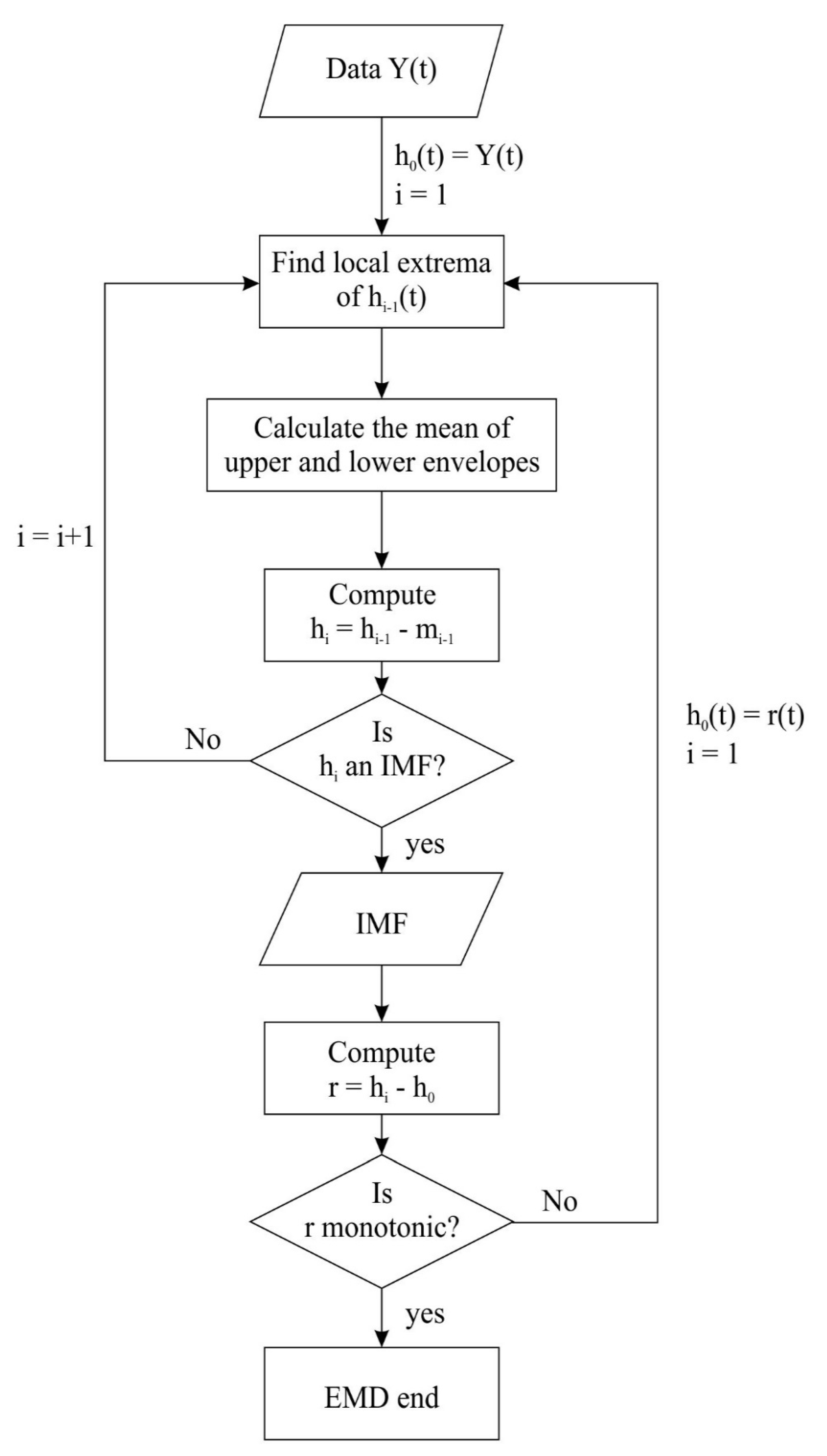
Figure 1. Flowchart for empirical mode decomposition.
Applsci 13 04572 g001
Figure 2. RF–IMF model.
Applsci 13 04572 g002
Figure 3. Rolling forecast model.
Applsci 13 04572 g003
Figure 4. Annual rainfall divided into training and testing datasets.
Applsci 13 04572 g004
Figure 5. A bar plot of the predicted and observed annual rainfall for ARMA model (0,0,2).
Applsci 13 04572 g005
Figure 6. Bar plot of the predicted and observed annual rainfall for random forest regression model.
Applsci 13 04572 g006
Figure 7. Plot of six IMFs from 1871 to 2020.
Applsci 13 04572 g007
Figure 8. A bar plot of the predicted and observed annual rainfall for RF–IMF model.
Applsci 13 04572 g008
Table 1. Pearson correlation coefficient matrix among original signal and the IMFs.
x(t)imf1imf2imf3imf4imf5imf6
x(t)1.000.770.360.280.180.230.03
imf10.771.000.11−0.03−0.05−0.08−0.05
imf20.360.111.000.090.000.000.03
imf30.28−0.030.091.000.03−0.100.00
imf40.18−0.050.000.031.000.080.00
imf50.23−0.082.00−0.100.081.000.17
imf60.03−0.00.000.000.030.171.00
Table 2. Actual rainfall and predicted rainfall values.
Year/ModelActual Rainfall (cm)ARMA (0,0,2) (cm)RF (cm) RF–IMF (cm)
2001263272281261
2002260292280294
2003231280247232
2004271280270259
2005230268269253
2006316274299265
2007313296283290
2008240280282266
2009258274257244
2010309286303307
2011278288281267
2012208258242225
2013319283281293
2014297299296302
2015256275274265
2016184280278202
2017267271264264
2018352295292337
2019312291271294
2020335276284291
Table 3. Comparison of different prediction models using Evaluation metrics.
Evaluation MetricsARMA (0,0,2)RFRF–IMF
MAE (cm)31.4526.6519.70
MSE (cm2)38.8026.6524.60
RMSE (cm)6.165.164.90
MAPE (%)12.3511.007.00
R20.280.380.76
Disclaimer/Publisher’s Note: The statements, opinions and data contained in all publications are solely those of the individual author(s) and contributor(s) and not of MDPI and/or the editor(s). MDPI and/or the editor(s) disclaim responsibility for any injury to people or property resulting from any ideas, methods, instructions or products referred to in the content.