Deep Learning-Assisted Transmit Antenna Classifiers for Fully Generalized Spatial Modulation: Online Efficiency Replaces Offline Complexity

Abstract

In this work, deep learning (DL)-based transmit antenna selection (TAS) strategies are employed to enhance the average bit error rate (ABER) and energy efficiency (EE) performance of a spectrally efficient fully generalized spatial modulation (FGSM) scheme. The Euclidean distance-based antenna selection (EDAS), a frequently employed TAS technique, has a high search complexity but offers optimal ABER performance. To address TAS with minimal complexity, we present DL-based approaches that reframe the traditional TAS problem as a classification learning problem. To reduce the energy consumption and latency of the system, we presented three DL architectures in this study, namely a feed-forward neural network (FNN), a recurrent neural network (RNN), and a 1D convolutional neural network (CNN). The proposed system can efficiently process and make predictions based on the new data with minimal latency, as DL-based modeling is a one-time procedure. In addition, the performance of the proposed DL strategies is compared to two other popular machine learning methods: support vector machine (SVM) and K-nearest neighbor (KNN). While comparing DL architectures with SVM on the same dataset, it is seen that the proposed FNN architecture offers a ~3.15% accuracy boost. The proposed FNN architecture achieves an improved signal-to-noise ratio (SNR) gain of ~2.2 dB over FGSM without TAS (FGSM-WTAS). All proposed DL techniques outperform FGSM-WTAS.

1. Introduction

The sixth-generation (6G) mobile communication system will be launched to fulfill unprecedented spectral efficiency (SE), energy efficiency (EE), massive connectivity, and latency demands that previous generations of networks could not meet [1,2,3]. These include a rise in connection density to 10 million devices per square kilometer, a doubling of SE to 100 b/s/Hz, and a notable decrease in latency to 0.1 ms.

In the past few years, several cutting-edge wireless communication technologies have been proposed, including index modulation (IM), intelligent reflecting surfaces (IRS), cognitive radio, multi-carrier modulation, and next-generation multiple access (NGMA). These technologies will eventually enable an increase in SE, improving quality of service (QoS), regardless of the wireless system used [4].

Wireless power transfer and simultaneous wireless information and power transfer are other effective ways to deliver energy to wireless receivers [5]. Cooperative and distributed multi-point transmissions can reduce the power requirement for dense cell-based communications. On the other hand, at the expense of increased latencies, relays and multi-hop transmissions can reduce power for long-distance communications. IRS configurations are presented and implemented in [6], where the results demonstrate that IRS improves the EE of the network. IM techniques can be incorporated to boost the network’s EE [1,5,7].

Massive multiple-input multiple-output (MIMO) is one of the methods used to enhance the SE in fifth-generation (5G) systems. A multi-antenna system leads to inter-antenna synchronization (IAS) and inter-channel interference (ICI) problems [7,8]. As the number of radio frequency (RF) chains grows, the hardware complexity of the system rises, leading to decreased EE. To address this issue, the idea of spatial modulation (SM) is presented [7]. In SM, a single antenna is operational at a time, which alleviates the burden on the RF chain. The SE of conventional SM is given as

$${{\xi }_{\mathit{SM}}=\log }_2\left(N_t\right)+{\log }_2\left(M\right),$$

(1)

Here, $N_t$ and M are used to represent the number of transmitting antennas and the order of the modulation, respectively. SE is limited in the SM system since it grows logarithmically with the number of transmitting antennas utilized. Therefore, more transmit antennas are needed to improve SE. Future-generation networks necessitate advanced SM variants to achieve the target SE requirements [8,9,10,11,12]. Based on their operational concept, advanced SM variants can transmit the same or different symbols over many antennas. Fully generalized spatial modulation (FGSM) and fully quadrature spatial modulation (FQSM) are two novel variants of SM in which the number of antennas employed at the transmitter is altered from one to multiple or all. Thus, the theoretical SE grows linearly with transmit antennas [12].

Additionally, as SM only uses a single antenna, it cannot accomplish transmit diversity [13,14,15]. In order to increase the signal-to-noise ratio (SNR) gains, transmit antenna selection (TAS) techniques are employed in the SM [13,14,15]. The receiver chooses the transmitter antenna subsets according to the channel quality information (CQI). In recent years, deep learning (DL), a new artificial intelligence (AI) method, has demonstrated its potential benefits in multiple areas, including speech processing, natural language processing, and image processing. A wide range of DL applications are being explored in physical-layer communications, including channel estimation, signal detection, beam prediction, etc. [16]. In this work, TAS is performed on FGSM using distinct machine learning (ML) and deep learning (DL) algorithms, whose efficacy is evaluated through classification accuracy and average bit error rate (ABER).

The manuscript is structured as follows: Section 2 examines related works and research gaps. Section 3 discusses the paradigms of FGSM and the Euclidean distance-based antenna selection (EDAS) scheme. Section 4 addresses the numerous DL algorithms employed in this study to implement FGSM-TAS as well as the complexity analysis of all proposed and traditional EDAS approaches. Section 5 compares the ABER performance of FGSM without TAS (FGSM-WTAS) and EDAS with all other suggested ML and DL algorithms using Monte–Carlo simulations. Lastly, Section 6 summarizes the work and proposes some areas for further investigation.

2. Related Works

Next-generation networks necessitate improvements in EE and SE [1,2,3,4,5]. The SE of SM has a logarithmic relationship with the number of transmit antennas, which degrades the SE performance of SM [8,9,10,11,12]. In [8,9,10,11,12], high-rate variants of SM are implemented to combat this issue. There are a number of potential variants of SM, such as enhanced spatial modulation (ESM) [8], generalized spatial modulation (GSM) [9], modified spatial modulation (MSM) [10], quadrature spatial modulation (QSM) [11], FGSM [12], and FQSM [12], etc. Transmit antennas and SE in FGSM and FQSM are linearly related, which satisfies the increasing SE requirements of 6G [12].

As the conventional SM does not provide transmit diversity gain [13,14,15,17], TAS schemes are incorporated to enhance transmit diversity. In [13,14,15,17], distinct open- and closed-loop TAS schemes for SM are introduced. Although EDAS provides the best ABER performance, its implementation is a challenging task. By combining transmit mode switching with adaptive modulation, a unique SM approach that maximizes channel utilization has been presented in [18]. This technique selects the subset of antennas with the lowest Euclidean distance (ED) between symbols. It is more computationally intensive due to the necessity of simultaneously finding antenna pairs and an order of constellation that maximizes minimum ED.

To resolve the issue of computational difficulty, antennas are selected on the basis of simple parameters such as channel gain, correlation angle, channel capacity, etc. The antenna subset with the highest channel capacity is selected using the capacity optimized antenna selection (COAS) approach [12,15]. When compared to EDAS, the performance of a TAS scheme that is based on COAS is found to be subpar. A TAS scheme based on correlation angle is discussed in [12,15], which evaluates the correlation angle between two antennas. The pair of antennas with the lowest correlation will be given precedence over the others. In [12,15], a capacity and correlation angle-based TAS strategy is suggested for improving ABER performance. This method can improve ABER performance at the cost of a noticeable increase in computational difficulty. Moreover, the system’s complexity is decreased by using a splitting strategy determined by capacity and correlation angle [12,15]. According to [15], EDAS is more effective than sub-optimal TAS approaches in SM and its variants. Furthermore, TAS schemes are incorporated in [12] to increase the transmit diversity gains of advanced variants of SM. In [12], the computational cost of EDAS is compared to other sub-optimal TAS approaches for FGSM in terms of real valued multiplications. According to this, the design of the EDAS approach is overly complex when compared to other methods.

In order to sidestep such tedious operations, a novel TAS method based on pattern recognition is presented in [19]. Here, support vector machine (SVM) and K-nearest neighbor (KNN) techniques are used for TAS, where the models were trained using 5000 samples each. It is possible to extend this work to incorporate more supervised ML/DL algorithms and larger datasets, which would improve the performance of the system. The effectiveness of these algorithms is evaluated using the element norm of H and the element norm of H^HH, which are two distinctive attributes of channel space. In [20], supervised ML techniques and deep neural networks (DNN) are presented and applied to address the issue of power allocation in adaptive SM-MIMO. Increasing the training set size beyond 2000 feature label pairs can improve its ABER performance. ML-based TAS methods are compared to SM without TAS (SM-WTAS) and EDAS in terms of ABER and computational complexity [21]. The SVM-based TAS scheme is less computationally complex than EDAS and does better than the classic SM with a minimum SNR gain of ~3.4 dB. This study can be extended by employing DL techniques in order to improve its accuracy even further. Because the computing complexity increases with the order of modulation and number of transmit antennas, the TAS algorithm is implemented with DNN for the MIMO system [22]. Algorithms for joint transmit and receive antenna selection (JTRAS) are suggested for SM systems, with the goal of optimizing both capacity and ED [23]. The authors of [23] used DL architectures for the basic SM, which are lacking in SE and may not be useful for future-generation networks. Later, DL methods are implemented to determine the optimal receive and transmit antenna configurations. In [24], DNN is used to implement the TAS algorithm for SM systems. To further improve the performance of the suggested technique, the processing load of the DNN is decreased by extracting the unique portion of the EDAS measure. In [25], a DL-based receiver model is implemented in which a DNN is used to do all of the information recovery tasks typically performed by a receiver, from decoding the incoming IQ signal to generating the final bit stream of data. Simulated findings reveal that the proposed DL model’s performance is comparable to that of an ideal soft ML decision and significantly better than that of the hard decision technique. In spite of this, ML and DL-based TAS algorithms have only been tested for fundamental SM, which may not meet SE demands.

These AI-based strategies have been developed and incorporated only for traditional MIMO and SM systems. To the best of our knowledge, no research study has given considerable attention to the problem of TAS employing DL for SM or advanced variants of SM. The primary contributions of the proposed work are as follows:

• There are no repositories that have the TAS dataset for FGSM. In total, two datasets of size 25,000 are created by applying the EDAS algorithm repeatedly. These datasets include information about channel setups and antenna counts for various MIMO configurations, as well as basic performance metrics such as ED.
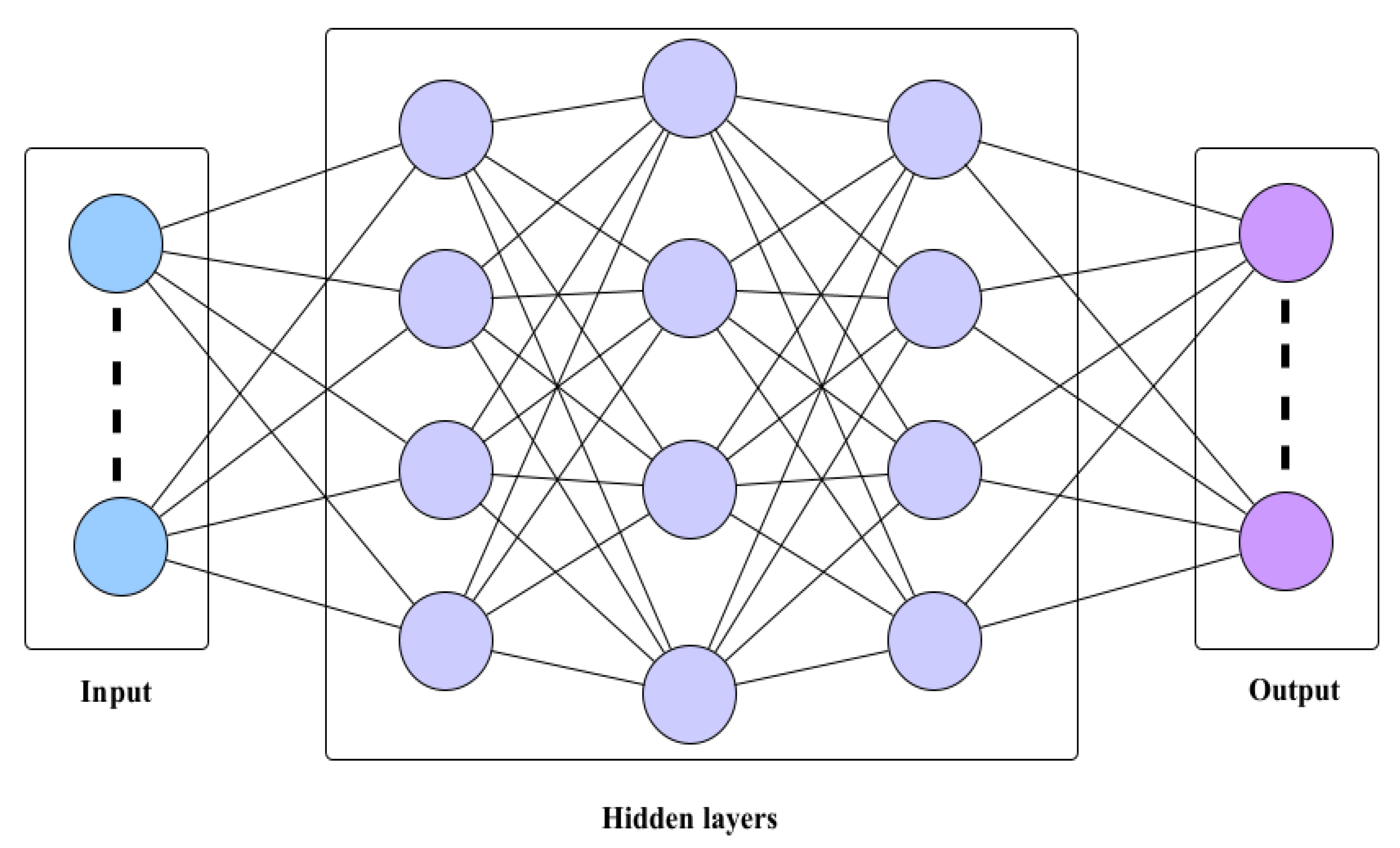
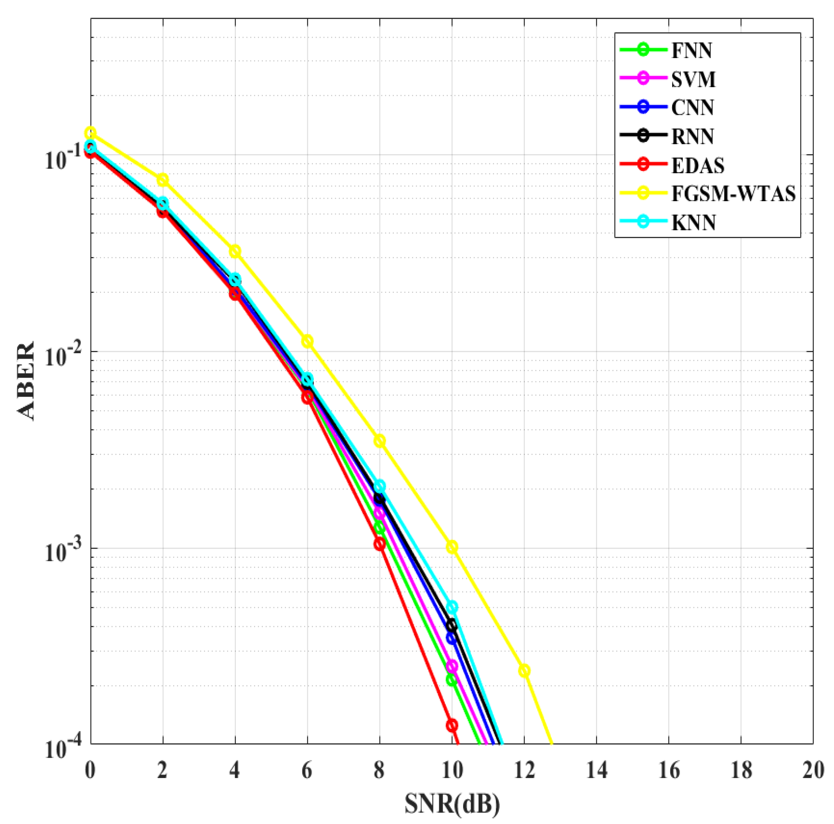
• Three distinct supervised DL methods are incorporated to demonstrate the improvements of DL over ML algorithms, including feed-forward neural networks (FNN), recurrent neural networks (RNN), and 1D convolutional neural networks (CNN).
• ML- and DL-based TAS methods are compared to WTAS and EDAS in terms of ABER and computational complexity.

3. System Model of FGSM and Traditional EDAS

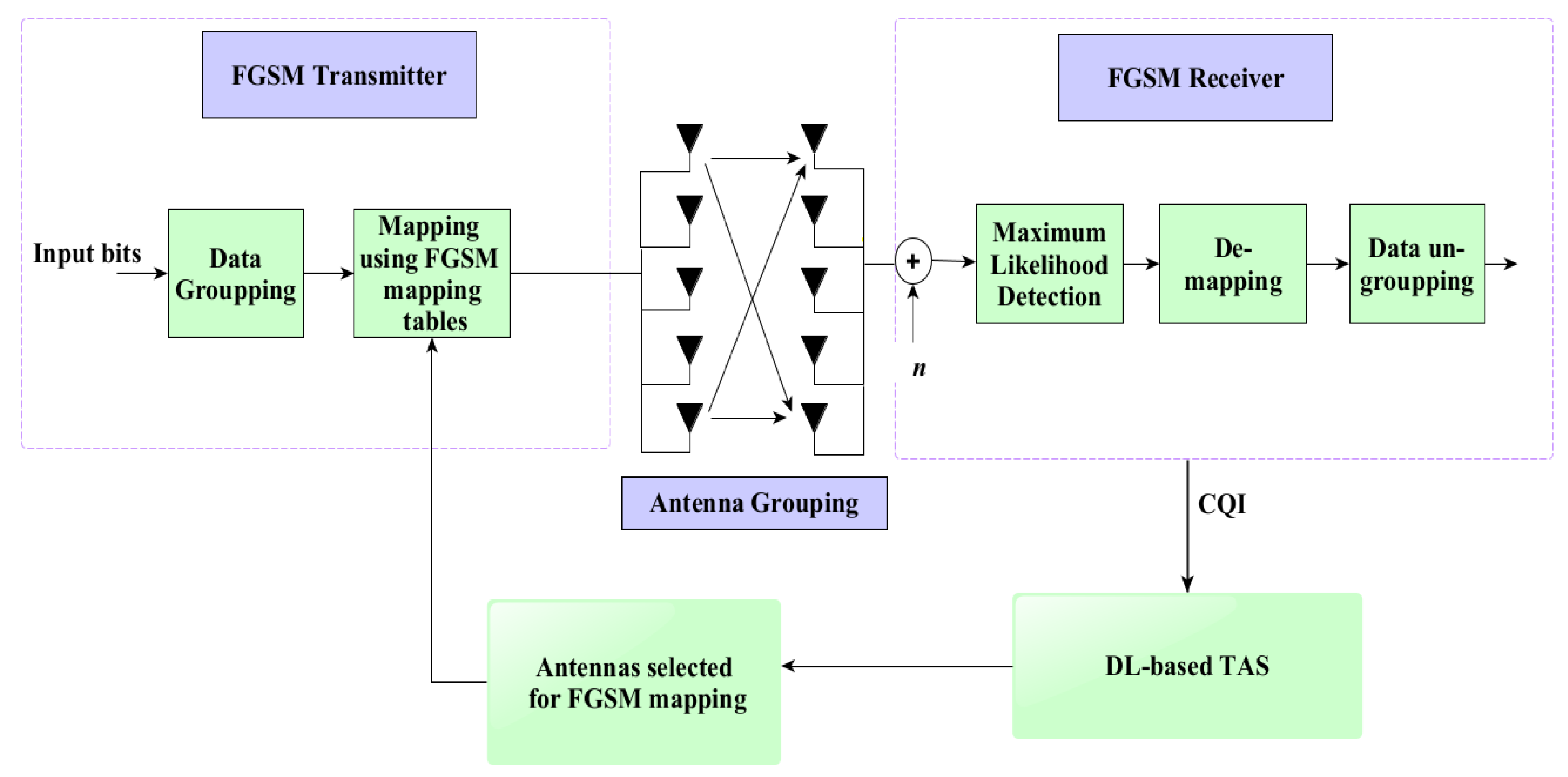
3.1. FGSM

An advanced variant of SM called FGSM enables the simultaneous transmission of the same symbol by one, many, or all antennas. Figure 1 depicts a simplified block diagram of the FGSM system. The index for the active antenna subset and the associated symbol to be transmitted are chosen in response to the incoming group of bits. Later, the maximum likelihood detector is applied to the received signal vector. The transmitted group of bits are reconstructed by demapping the detected transmit antenna indices and their associated transmitted symbol.

In comparison to the SM, the SE is linearly proportional to the number of transmitting antennas, which enhances the SE. The SE of the FGSM is estimated as follows [12]:

$${\xi }_{FGSM}=\left(N_t-1\right){+\log }_2\left(M\right)$$

(2)

A sample FGSM mapping for $N_t$ = 4 and $M$ = 2 is displayed in

Table 1. FGSM mapping for $N_t$ = 4 and $M$ = 2.

Sr. No.	Input Bits	Antenna Set	Symbols	Transmit Vector
1	0000	1, 2	−1	𝟆 = [−1, −1, 0, 0]
2	0001	1, 2	+1	𝟆 = [1, 1, 0, 0]
3	0010	1, 3	−1	𝟆 = [−1, 0, −1, 0]
4	0011	1, 3	+1	𝟆 = [1, 0, 1, 0]
5	0100	1, 4	−1	𝟆 = [−1, 0, 0, −1]
6	0101	1, 4	+1	𝟆 = [1, 0, 0, 1]
7	0110	2, 3	−1	𝟆 = [0, −1, −1, 0]
8	0111	2, 3	+1	𝟆 = [0, 1, 1, 0]
9	1000	2, 4	−1	𝟆 = [0, −1, 0, −1]
10	1001	2, 4	+1	𝟆 = [0, 1, 0, 1]
11	1010	3, 4	−1	𝟆 = [0, 0, −1, −1]
12	1011	3, 4	+1	𝟆 = [0, 0, 1, 1]
13	1100	1, 2, 3	−1	𝟆 = [−1, −1, −1, 0]
14	1101	1, 2, 3	+1	𝟆 = [1, 1, 1, 0]
15	1110	2, 3, 4	−1	𝟆 = [0, −1, −1, −1]
16	1111	2, 3, 4	+1	𝟆 = [0, 1, 1, 1]

. Let the grouped bits be [0 1 0 1], where the first $\left(N_t-1\right)$ bit, i.e., [0 1 0] refers to the antenna combination (1, 4) and the last ${\log }_2\left(M\right)$ bit, i.e., [1], corresponds to the transmitted symbol +1. The accompanying transmit vector is given by 𝟆 = [1, 0, 0, 1].

Additive white Gaussian noise (AWGN) n and multipath channel H have an effect on the transmit vector 𝟆. The FGSM receiver employing maximum likelihood detection is elaborated in [12].

3.2. EDAS

TAS improves the transmit diversity of traditional MIMO and SM systems, as described in Section 2. EDAS is the most popular and optimal TAS technique, with the objective of choosing antenna combinations that enhance the minimum ED of received constellations. It is shown that EDAS has superior EE and ABER compared to other conventional methods [12,15]. The channel matrix H is derived from H_T when TAS is incorporated in FGSM. The important steps in the EDAS process are listed below:

(1)

Determine the total number of distinct feasible subsets $N_p$ = $\left(\begin{array}{c}{N}_T\\ N_t\end{array}\right)$.

(2)

Find all of the possible transmit vectors $2^{{\xi }_{FGSM}}$ for each antenna subset.

(3)

For each antenna subset, calculate their least possible ED using:

$$\mathsf{\lambda }=\left(\underset{{\mathsf{\varkappa }}_j\ne {\mathsf{\varkappa }}_k\in \mathcal{X}}{\mathrm{m}\mathrm{i}\mathrm{n}}{‖{\mathit{H}}_{\mathit{T}}\left({\mathsf{\varkappa }}_j-{\mathsf{\varkappa }}_k\right)‖}^2\right)$$

(3)

In (3), $\mathcal{X}$ represents the set of all possible transmit vectors.

(4)

Determine the subset of antennas with the maximum ED.

$$\widehat{c}=\underset{c\in \mathrm{1,2} \dots {\mathit{N}}_p}{\mathrm{arg\; max}}\lambda ,$$

(4)

here $\mathsf{\lambda }=\left[{\mathsf{\lambda }}_1,{\mathsf{\lambda }}_2 \dots {\mathsf{\lambda }}_{N_p}\right]$.

On the basis of the antenna subset index acquired in step 4, the antenna indices and their corresponding $N_r$ x $N_t$ channel matrix $\left(\mathit{H}\right)$ are computed.

4. Design and Complexity of Proposed DL Architectures

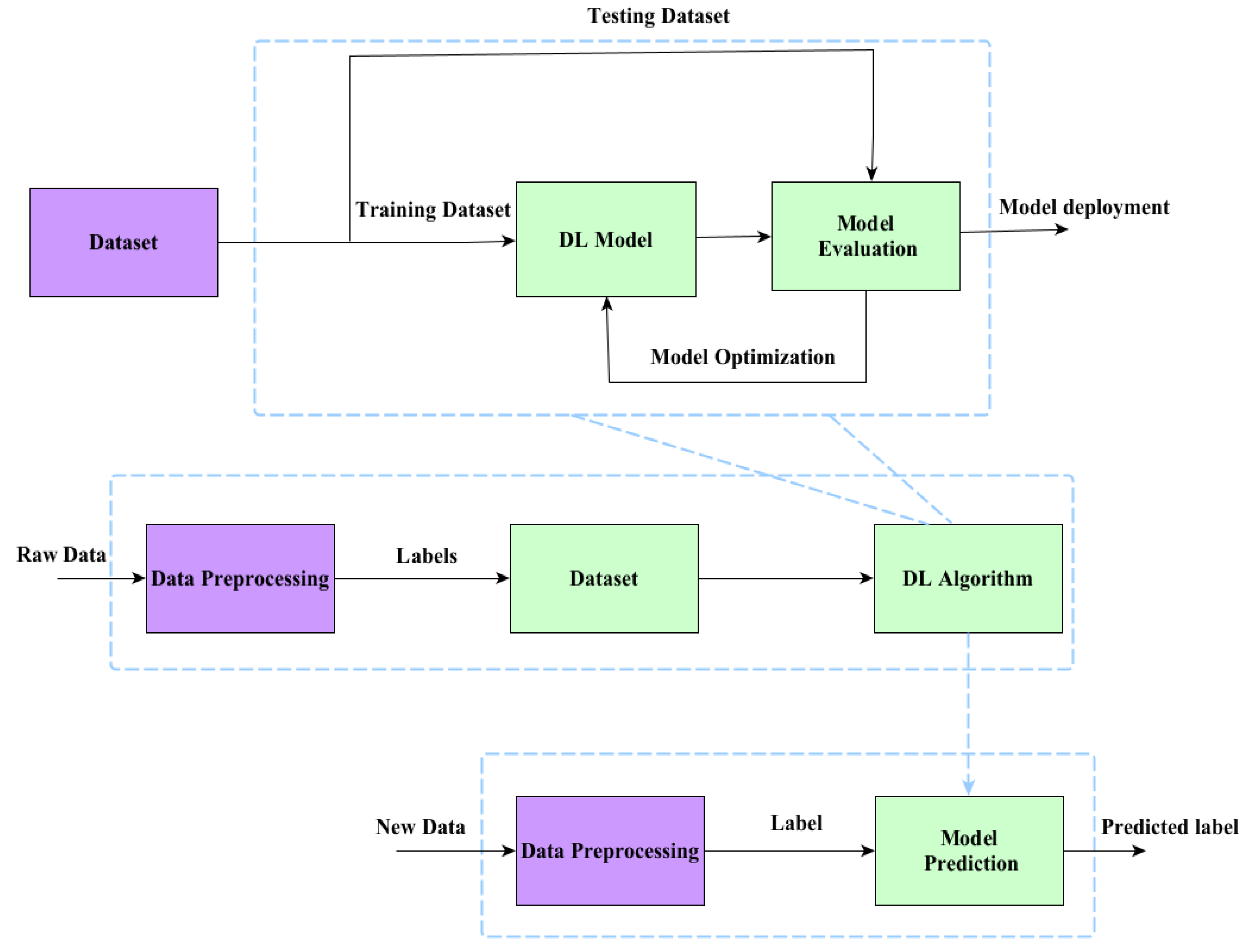
4.1. DL-Based TAS Schemes for FGSM

In this study, DL-based techniques are used to perform TAS in FGSM. Figure 2 shows the DL-based classification learning architecture for TAS. The primary steps followed by these DL architectures are shown in Figure 3. First, the data is pre-processed using the mean normalization technique. DL-based systems require real-valued training datasets, while MIMO channel coefficients are complex in nature. From the pre-processed data, real-valued features are retrieved. Lastly, different DL techniques are used to train the model based on the specified features and class labels. The trained networks are used to make predictions about the classes based on the new data. $N_t$ antennas are selected from $N_T$ based on the class labels obtained from DL algorithms if CQI is present at the target device.

An input vector is required to represent the channel coefficients since antenna combinations are classified against an input array. Following is a brief summary of the steps involved in the acquisition of datasets:

i.

Dataset generation: $N_c$ random channel matrices ${\mathit{H}}_{\mathrm{q}}ϵC^{N_r\times N_T}$, $q\in 1\cdots$ $N_c$ are generated to create the dataset.

$$\mathrm{Ḧ}={[{\mathit{H}}_1,{\mathit{H}}_2,{\cdots ,\mathit{H}}_{N_c}]}^T$$

(5)

$\mathrm{Ḧ}$ consists of all these $N_c$ records or channel matrices.

ii.

Feature vector extraction: This work utilized the absolute values of every element of the channel matrix as an input feature with size $N_{\mathrm{f}}=N_r\times N_T$. The resulting feature vector is given by:

$${\mathit{f}}^{\mathrm{q}}={[\left|h_{\mathrm{1,1}}^q\right|,\cdots ,\left|h_{1,N_T}^q\right|,\cdots ,\left|h_{j,k}^q\right|,\cdots ,\left|h_{N_r,N_T}^q\right|]}^T$$

(6)

here $h_{j,k}^q$ is the (j, k)th element of ${\mathit{H}}_{\mathrm{q}}$, its absolute value is given as:

$$\left|h_{j,k}^q\right|=\sqrt{\mathfrak{R}{\left(h_{j,k}^q\right)}^2+\mathfrak{I}{\left(h_{j,k}^q\right)}^2}$$

(7)

The mean normalization is performed to avoid the effect of bias [21].

$$v^{\mathrm{q}}\left(\mathrm{n}\right)=\frac{\left(f^{\mathrm{q}}\right(\mathrm{n})-\mathrm{mean}\left(\mathit{f}\right(n)))}{\left(\max \left(\mathit{f}\right(n\left)\right)-\min \left(\mathit{f}\right(n\left)\right)\right)},n\in 1\cdots N_f,q\in 1\cdots N_c$$

(8)

iii.

Calculation of KPI: (3) is used to evaluate ED, which is considered the key performance indicator (KPI) in this study. The KPI is utilized to label the dataset.

iv.

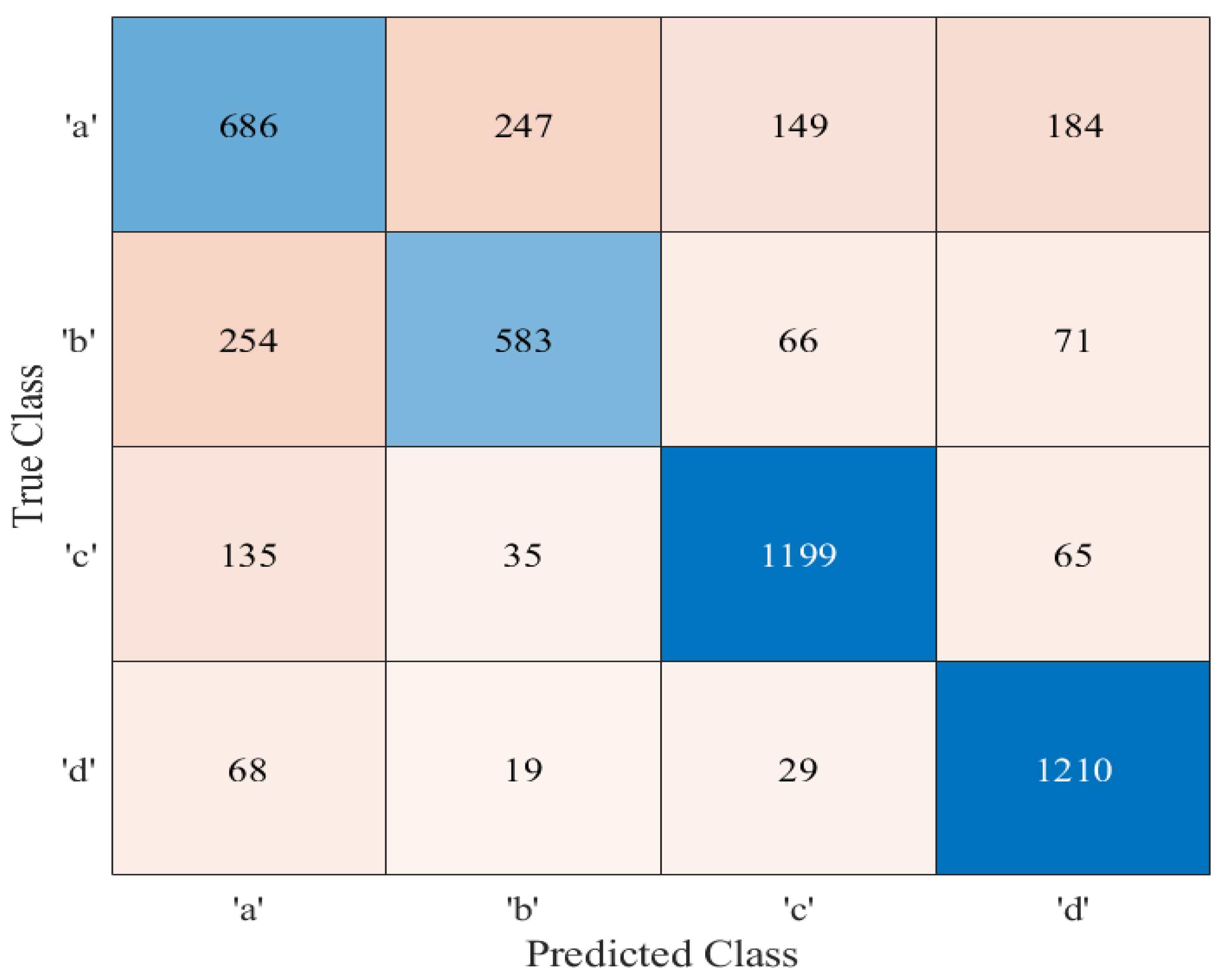
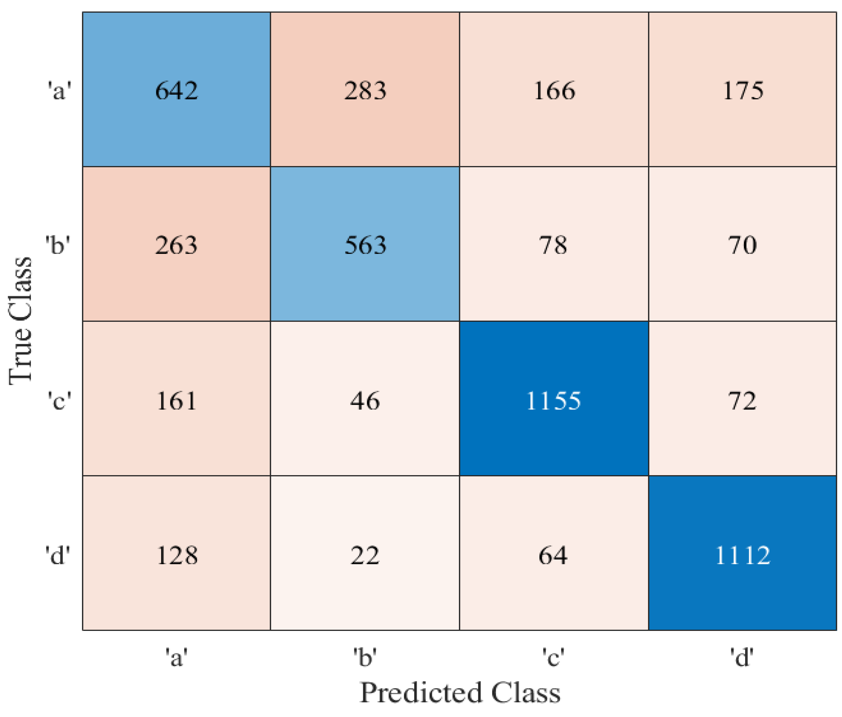
Class labeling: There is a unique label associated with every antenna subset. Antenna subset and class label mapping examples for the configurations $N_r=4$, $N_t=$ 3, and $N_T=4$ is given in

Table 2. Antenna subset-class label mapping for $N_r=4$, $N_t=$ 3, and $N_T=4$.

Labels	Antenna Subsets
a	${\beta }_1=[$1, 2, 3]
b	${\beta }_2=[$1, 2, 4]
c	${\beta }_3=[1,3,4]$
d	${\beta }_4=[2,3,4]$

.

4.2. DL Architecture

Figure 4 shows the proposed DL architecture. First, the FNN is utilized so that any nonlinear function can be learned. RNN is also included because FNN was incapable of identifying sequential information in the input data. In contrast, CNN is investigated because it reveals the spatial features of the input data more effectively.

All proposed DL networks have L layers: an input layer, L-2 hidden layers, and an output layer. Full-connected (FC) layers are chosen as the hidden layers for FNN. Let ${\widehat{\mathit{r}}}^{\mathrm{q}}$ be the output vector at the last layer. The number of neurons utilized at every layer is denoted by $N_l,$ $l\in 0\cdots L-1$. A normalized feature vector ${\mathit{v}}^{\mathrm{q}}$ of size $N_f$ is sent from the input layer to the first hidden layer for further processing, which is processed as [26].

$${\widehat{\mathit{r}}}_1^q={max(\mathit{W}}_1{\mathit{v}}^{\mathrm{q}}+{\mathit{b}}_1,0)$$

(9)

where the output vector of the first hidden layer is represented by ${\mathit{r}}_1^q$. Both the weight matrix and the bias vector associated with the first hidden layer are denoted by ${\mathit{W}}_1$ and ${\mathit{b}}_1$, respectively. The rectified linear unit (ReLU) activation function is utilized at the hidden layers. The output of the ReLU activation function is given by:

$$f_{ReLU}\left(s\right)=max(0,s)$$

(10)

The output vector of the $l$th hidden layer is given as [26]

$${\widehat{\mathit{r}}}_l^q={max(\mathit{W}}_l{\widehat{\mathit{r}}}_{l-1}^q+{\mathit{b}}_l,0)$$

(11)

where the weight matrix and the bias vector associated with the $l$th hidden layer are denoted by ${\mathit{W}}_l$ and ${\mathit{b}}_l$.

The FC layer is used as an output layer for all proposed networks. The number of neurons utilized at the output layer corresponds to the number of class labels (N_p). The Softmax activation function ($\delta$) is employed at the output layer to perform the multiclass classification task. The output vector of the $L-1$ layer is given by [26]

$${\widehat{\mathit{r}}}_{L-1}^q={\delta (\mathit{W}}_{L-1}{\widehat{\mathit{r}}}_{L-2}^q+{\mathit{b}}_{L-1},0)$$

(12)

where the weight matrix and the bias vector associated with the output layer are denoted by ${\mathit{W}}_{L-1}$ and ${\mathit{b}}_{L-1}$.

On the basis of the procedure described above, the entire training mapping rule is given as [26]

$${\widehat{\mathit{r}}}^{\mathrm{q}}={\delta (\mathit{W}}_{L-1}{\left(max\right({\mathit{W}}_{L-2}\cdots (\mathit{W}}_1{\mathit{v}}_1^q+{\mathit{b}}_1,0)\cdots +{\mathit{b}}_{L-2},0))+{\mathit{b}}_{L-1})$$

(13)

We use (8) to acquire the feature vector ${\mathit{f}}_N$ for a new observation ${\mathit{H}}_N$ and the label is retrieved from (13). According to Figure 5a, the classification layer receives its inputs from the output layer via the Softmax layer.

Long short-term memory (LSTM) is employed as the hidden layer in the RNN architecture. There are three multiplicative units (input gate, forget gate, and output gate) that make up the memory module of a RNN using the LSTM architecture. For any LSTM unit, given its input and output values (${\mathit{x}}_{l-1}$ and ${\mathit{x}}_l$, respectively), the relationship between them at time step t is stated as [27].

$${\mathit{f}}_l^t=f_{ReLU}{(\mathit{W}}_f{\mathit{x}}_l^{t-1}+{\mathit{Z}}_f{\mathit{x}}_l^t+{\mathit{b}}_f)$$

(14)

$${\mathit{i}}_l^t=f_{ReLU}{(\mathit{W}}_i{\mathit{x}}_l^{t-1}+{\mathit{Z}}_i{\mathit{x}}_l^t+{\mathit{b}}_i)$$

(15)

$${\mathit{o}}_l^t=f_{ReLU}{(\mathit{W}}_o{\mathit{x}}_l^{t-1}+{\mathit{Z}}_o{\mathit{x}}_l^t+{\mathit{b}}_o)$$

(16)

$${{\mathit{c}}_l^t=\mathit{f}}_l^t\odot {\mathit{c}}_l^{t-1}+{\mathit{i}}_l^t\odot {\sigma }_c{(\mathit{W}}_c{\mathit{x}}_l^{t-1}+{\mathit{Z}}_c{\mathit{x}}_l^t+{\mathit{b}}_c)$$

(17)

$${{\mathit{x}}_L^t=\mathit{o}}_l^t\odot {\sigma }_z{\mathit{c}}_l^t$$

(18)

where ${\mathit{f}}_l^t$, ${\mathit{i}}_l^t$, and ${\mathit{o}}_l^t$ represent, input and output gate vectors. Parameter matrices and vectors associated with these gates are denoted by $\mathit{W}$, $\mathit{Z}$, and $\mathit{b},$ respectively. The unit state of LSTM is denoted by ${\mathit{c}}_l^t$. Both ${\sigma }_c$ and ${\sigma }_z$ are hyperbolic tangents, and the Hadamard product is denoted by the $\odot$ operator. In both FNN and RNN architectures, three hidden layers are utilized. In these three hidden layers, there are 256, 128, and 128 neurons, respectively. The proposed RNN architecture is depicted in Figure 5b. All of the proposed DL architectures are trained with the help of the adaptive moment optimizer (Adam).

Similarly, a 1D convolution layer is selected as the hidden layer for CNN architecture. The output at the $l$th hidden layer in 1D CNN is given as [28]

$${\widehat{\mathit{r}}}_L^q=f_{ReLU}\left({\mathit{b}}_l^i+\sum _{j=1}^{N_l}conv1D\left({\mathit{W}}_l^{ij},{\mathit{s}}_l^j\right)\right)$$

(19)

where the kernel and the bias associated with the $l$th hidden layer for its ith neuron are denoted by ${\mathit{W}}_l^{ij}$ and ${\mathit{b}}_l^i$. Output of the jth neuron is represented by ${\mathit{s}}_l^j$. The proposed architecture of 1D CNN is shown in Figure 5c, and its parameters are listed in

Table 3. List of parameters of the proposed CNN architecture.

Parameters	Values
Number of hidden layers	3
1D convolution layer 1	Filter Size = 3/Number of filters = 32
1D convolution layer 2	Filter Size = 6/Number of filters = 32
1D convolution layer 3	Filter Size = 9/Number of filters = 32
Activation function	ReLU
Optimizer	Adam

.

4.3. Complexity of Proposed DL-Based TAS Schemes

Table 4. Comparison of several TAS techniques in terms of order of complexity.

DL-Based TAS Scheme	Order of Complexity	Configuration 1 ${\mathit{N}}_{\mathit{t}}={\mathit{N}}_{\mathit{r}}=8$, ${\mathit{N}}_{\mathit{T}}=10$, $\mathit{M}=4$	Configuration 2 ${\mathit{N}}_{\mathit{t}}={\mathit{N}}_{\mathit{r}}=8$, ${\mathit{N}}_{\mathit{T}}=10$, $\mathit{M}=64$
Traditional EDAS	$\mathrm{O}\left(N_P{2}^{{\xi }_{FGSM}}\right(2^{{\xi }_{FGSM}}-1\left)8N_r\right)$ [12]	O(0.753 × 109)	O(12.07 × 109)
FNN-based TAS	$\mathrm{O}\left(N_0{N}_1{N}_2\right)$ [23]	O(4.194 × 106)	O(4.194 × 106)
RNN-based TAS	$\mathrm{O}\left(N_0{N}_1{N}_2\right)$ [23]	O(4.194 × 106)	O(4.194 × 106)
1D CNN-based TAS	$\mathrm{O}({FS}_0{FS}_1{FS}_2$) [23]	O(5.308 × 106)	O(5.308 × 106)

presents the computational complexity analysis of the proposed DL-based systems and traditional EDAS for FGSM. The computational complexity of traditional EDAS is given in [12], while the computational complexity of the proposed DL-based systems is presented in [23]. Both measures are expressed in terms of real valued multiplication. In general, the order of complexity of an RNN or FNN is determined by the number of neurons present in each layer ${(N}_l,$ $l\in 0\cdots L-1)$ and number of hidden layers ($L$); whereas, the order of complexity of a CNN is determined by the number of filters and filter size present (${FS}_l=$ (No. of filters $\times$ filter size) for lth layer) [23]. As can be seen from Table 3, the computational complexity of traditional EDAS grows in proportion to the modulation order and the number of transmit and receive antennas. On the other hand, the complexity of the proposed DL algorithms is unaffected by the different configurations of the system and remains the same throughout. Every random channel matrix sample is processed using the traditional EDAS, and the corresponding antenna indices are saved. During offline training, the features are extracted from the random channel matrix, and the label associated with the antenna index recorded utilizing EDAS is used to train the model. Training requires these computations, and this is a one-time task. Once the model has been trained for the unseen data sample, it will use its prior knowledge to make a prediction about the class label. This simplifies things online and reduces the system’s complexity. With an increasing number of these components, traditional EDAS becomes more complex; therefore, DL approaches for TAS are needed to simplify it.

5. Discussion on Simulation Results

The proposed DL architectures have been implemented and evaluated in MATLAB R2022b using the deep network designer application.

Table 5. List of parameters used for system implementation.

Parameters	Values
Dataset Size ($N_c$)	25,000
Holdout ratio	80–20%
Mini batch size	64
Maximum epochs	50
Initial learning rate	0.00012
Optimizer	Adam
Learning drop rate factor	0.15
Target ABER	${10}^{-4}$

outlines all of the important simulation settings. There is no dataset in any of the repositories for TAS-assisted FGSM. As the use of SE increases, so does the computing complexity of traditional EDAS. As a result, we planned to employ DL architectures by benchmarking the optimal EDAS method and creating datasets with it. The EDAS algorithm is repeatedly executed for each of the configurations listed in

Table 6. Configurations of generated datasets.

Dataset	Configurations	Size
Dataset 1	$N_{\mathrm{T}}$ = 4, $N_{\mathrm{t}}$ = 3, $N_{\mathrm{r}}=$ 4, M = 4	25,000
Dataset 2	$N_{\mathrm{T}}$ = 4, $N_{\mathrm{t}}$ = 3, $N_{\mathrm{r}}=$ 4, M = 16	25,000

to generate two different datasets of size 25,000. The label is provided by the EDAS antenna indices, and the inputs (features) are derived from the random channel matrix. This is a one-time process, and the computations are required during the offline training phase. The features such as $\mathfrak{R}$($h_{ij}$), ℑ($h_{ij}$), ∡($h_{ij}$), ${\left|h_{ij}\right|}^2,$ and the squared element norm of (H^HH) are ignored due to their poor accuracy. As discussed in Section 4.1, $\left|h_{ij}\right|$ is used to train the model because of its higher accuracy. The classification accuracy of these proposed algorithms has been tested on 80% of holdouts. Because increasing the batch size reduces accuracy, we set the batch size at 32.

The training process associated with FNN is displayed in Figure 6. This figure shows that the network converges after 50 epochs with an average accuracy of 73.56%. This implies that ~73% of the channels were accurately predicted, providing the same predictions as conventional EDAS. As training progresses, the training loss decreases or stabilizes, proving the convergence of the models. At the end of training, the training and validation losses are almost identical. There are 312 batches for every epoch (20,000/64 = 312) [29,30]. The algorithm will run through 312 cycles every epoch, passing each batch in turn. Since, the total number of epochs is set to 50, there are a total of 15,600 iterations (312 $\times$ 50 = 15,600). A similar decreasing trend can be observed in both, and once the minimum has been reached, they do not rise again. One of the criteria that is utilized in the assessment of a classification model is its accuracy. This refers to the trained model’s percentage of accurate classifications. To determine the accuracy of the proposed DL architecture, a confusion matrix is used. The confusion matrix of the proposed FNN architecture is depicted in Figure 7. The entries on the diagonal are the correct values identified by the FNN architecture. The other entries correspond to the number of incorrect predictions. Figure 7 shows that when the trained FNN architecture is tested on a dataset of 5000 samples, it correctly predicts 3678 of them.

Figure 8 and Figure 9 represent the training process and confusion matrix for the proposed RNN architecture. According to Figure 8, after 50 epochs, the network achieves an average accuracy of 69.44%. Similarly, the training process and confusion matrix of 1D CNN are displayed in Figure 10 and Figure 11. From Figure 10, it is evident that after 50 epochs, the network is able to reach an average accuracy of 70.32%.

In Figure 12, the ABER performance of proposed DL-based schemes is examined with WTAS, traditional EDAS, and two widely used ML algorithms, SVM and KNN, for $N_T$ = 4, $N_t$ = 3, $N_r$ = 4, and M = 4. It is observed that, after the traditional EDAS, the proposed FNN-based TAS scheme outperforms SVM, KNN, and other DL-based systems. When compared to the FGSM-WTAS method, the FNN-based TAS scheme reduces the SNR requirement by ~2 dB. Due to its higher classification accuracy, the ABER performance of FNN-based TAS is superior to other DL-based TAS schemes. When compared to [19], the disparity between the traditional EDAS scheme and the proposed method using SVM to achieve an ABER of ${10}^{-4}$ is ~7 dB, which is very large. In our case, the margin between the proposed FNN scheme and traditional EDAS scheme is smaller (~0.6 dB), indicating a significant improvement in the system’s overall performance. Using the proposed FNN DL architecture, we obtained a ~3.2% enhancement compared to the SVM proposed in [21].

This performance is re-evaluated in Figure 13 by varying the constellation order to 16. All DL-based methods as well as SVM and KNN require higher SNRs for larger values of M. Both FGSM-WTAS and conventional EDAS require greater SNR than the previous configuration. The SNR demand is increased by ~1.53 dB for FGSM-WTAS and ~1.74 dB for standard EDAS. In this case as well, FNN outperforms FGSM-WTAS by ~2.2 dB.

6. Conclusions

In this work, three different DL-based TAS techniques for FGSM are proposed and implemented. The ABER performance of the recommended algorithms is compared to that of EDAS and WTAS for different configurations of $N_T$, $N_{\mathrm{t}}$, and M. The percentage of classification accuracy and simulations show that the FNN-based TAS scheme outperforms the other DL-based TAS methods and SVM and KNN as well. If the number of features and dataset size are larger, then 1D CNN and RNN may perform better than FNN. EDAS has better ABER performance than FNN; however, FNN-based TAS schemes are more efficient computationally. This makes it a potential option for next-generation networks. In the future, IRS could be integrated into communication systems. The proposed DL architectures can be employed for TAS in high-rate SM variants such as FQSM.

References

1. Hong, E.-K.; Lee, I.; Shim, B.; Ko, Y.-C.; Kim, S.-H.; Pack, S.; Lee, K.; Kim, S.; Kim, J.-H.; Shin, Y.; et al. 6G R&D vision: Requirements and candidate technologies. J. Commun. Netw. 2022, 24, 232–245. [Google Scholar]
2. Dang, S.; Amin, O.; Shihada, B.; Alouini, M.-S. What should 6G be? Nat. Electron. 2020, 3, 20–29. [Google Scholar] [CrossRef]
3. Rekkas, V.P.; Sotiroudis, S.; Sarigiannidis, P.; Wan, S.; Karagiannidis, G.K.; Goudos, S.K. Machine learning in beyond 5G/6G networks—State-of-the-art and future trends. Electronics 2021, 10, 2786. [Google Scholar] [CrossRef]
4. Liu, Y.; Zhang, S.; Mu, X.; Ding, Z.; Schober, R.; Al-Dhahir, N.; Hossain, E.; Shen, X. Evolution of NOMA toward next generation multiple access (NGMA) for 6G. IEEE J. Sel. Areas Commun. 2022, 40, 1037–1071. [Google Scholar] [CrossRef]
5. Guan, G.; Liu, M.; Tang, F.; Kato, N.; Adachi, F. 6G: Opening new horizons for integration of comfort, security, and intelligence. IEEE Wirel. Commun. 2020, 27, 126–132. [Google Scholar]
6. Basar, E. Transmission through large intelligent surfaces: A new frontier in wireless communications. In Proceedings of the 2019 European Conference on Networks and Communications (EuCNC), Valencia, Spain, 18–21 June 2019; IEEE: Piscataway, NJ, USA, 2019; pp. 112–117. [Google Scholar]
7. Ertugrul, B.; Wen, M.; Mesleh, R.; Di Renzo, M.; Xiao, Y.; Haas, H. Index modulation techniques for next-generation wireless networks. IEEE Access 2017, 5, 16693–16746. [Google Scholar]
8. Chien-Chun, C.; Sari, H.; Sezginer, S.; Su, T.Y. Enhanced spatial modulation with multiple signal constellations. IEEE Trans. Commun. 2015, 63, 2237–2248. [Google Scholar]
9. Abdelhamid, Y.; Mesleh, R.; Di Renzo, M.; Haas, H. Generalised spatial modulation for large-scale MIMO. In Proceedings of the 2014 22nd European Signal Processing Conference (EUSIPCO), Lisbon, Portugal, 1–5 September 2014; IEEE: Piscataway, NJ, USA, 2014; pp. 346–350. [Google Scholar]
10. Gaurav, J.; Gudla, V.V.; Kumaravelu, V.B.; Reddy, G.R.; Murugadass, A. Modified spatial modulation and low complexity signal vector based minimum mean square error detection for MIMO systems under spatially correlated channels. Wirel. Pers. Commun. 2020, 110, 999–1020. [Google Scholar]
11. Raed, M.; Ikki, S.S.; Aggoune, H.M. Quadrature spatial modulation. IEEE Trans. Veh. Technol. 2014, 64, 2738–2742. [Google Scholar]
12. Vardhan, G.V.; Kumaravelu, V.B.; Murugadass, A. Transmit antenna selection strategies for spectrally efficient spatial modulation techniques. Int. J. Commun. Syst. 2022, 35, e5099. [Google Scholar]
13. Rakshith, R.; Hari, K.V.S.; Hanzo, L. Antenna selection in spatial modulation systems. IEEE Commun. Lett. 2013, 17, 521–524. [Google Scholar]
14. Narushan, P.; Xu, H. “Comments on” antenna selection in spatial modulation systems. IEEE Commun. Lett. 2013, 17, 1681–1683. [Google Scholar]
15. Hindavi, J.; Kumaravelu, V.B. Transmit Antenna Selection Assisted Spatial Modulation for Energy Efficient Communication. In Proceedings of the 2021 Innovations in Power and Advanced Computing Technologies (i-PACT), Kuala Lumpur, Malaysia, 27–29 November 2021; IEEE: Piscataway, NJ, USA, 2021; pp. 1–5. [Google Scholar]
16. Bo, L.; Gao, F.; Zhang, S.; Zhou, T.; Alkhateeb, A. Deep learning-based antenna selection and CSI extrapolation in massive MIMO systems. IEEE Trans. Wirel. Commun. 2021, 20, 7669–7681. [Google Scholar]
17. Narushan, P.; Xu, H. Low-complexity transmit antenna selection schemes for spatial modulation. IET Commun. 2015, 9, 239–248. [Google Scholar]
18. Ping, Y.; Xiao, Y.; Li, L.; Tang, Q.; Yu, Y.; Li, S. Link adaptation for spatial modulation with limited feedback. IEEE Trans. Veh. Technol. 2012, 61, 3808–3813. [Google Scholar]
19. Ping, Y.; Zhu, J.; Xiao, Y.; Chen, Z. Antenna selection for MIMO system based on pattern recognition. Digit. Commun. Netw. 2019, 5, 34–39. [Google Scholar]
20. Ping, Y.; Xiao, Y.; Xiao, M.; Guan, Y.L.; Li, S.; Xiang, W. Adaptive spatial modulation MIMO based on machine learning. IEEE J. Sel. Areas Commun. 2019, 37, 2117–2131. [Google Scholar]
21. Kishor, J.H.; Kumaravelu, V.B. Transmit antenna selection for spatial modulation based on machine learning. Phys. Commun. 2022, 55, 101904. [Google Scholar]
22. Meenu, K. Deep learning based low complexity joint antenna selection scheme for MIMO vehicular adhoc networks. Expert Syst. Appl. 2023, 219, 119637. [Google Scholar]
23. Gökhan, A.; Arslan, İ.A. Joint transmit and receive antenna selection for spatial modulation systems using deep learning. IEEE Commun. Lett. 2022, 26, 2077–2080. [Google Scholar]
24. Ahmet, A.İ.; Altin, G. A novel deep neural network based antenna selection architecture for spatial modulation systems. In Proceedings of the 2021 56th International Scientific Conference on Information, Communication and Energy Systems and Technologies (ICEST), Sozopol, Bulgaria, 16–18 June 2021; IEEE: Piscataway, NJ, USA, 2021; pp. 141–144. [Google Scholar]
25. Shilian, Z.; Chen, S.; Yang, X. DeepReceiver: A deep learning-based intelligent receiver for wireless communications in the physical layer. IEEE Trans. Cogn. Commun. Netw. 2020, 7, 5–20. [Google Scholar]
26. Abeer, M.; Bai, Z.; Oloruntomilayo, F.-P.; Pang, K.; Yang, Y.; Zhou, D.; Kwak, K.S. Low complexity deep neural network based transmit antenna selection and signal detection in SM-MIMO system. Digit. Signal Process. 2022, 130, 103708. [Google Scholar]
27. Jianfeng, Z.; Mao, X.; Chen, L. Speech emotion recognition using deep 1D & 2D CNN LSTM networks. Biomed. Signal Process. Control. 2019, 47, 312–323. [Google Scholar]
28. Serkan, K.; Avci, O.; Abdeljaber, O.; Ince, T.; Gabbouj, M.; Inman, D.J. 1D convolutional neural networks and applications: A survey. Mech. Syst. Signal Process. 2021, 151, 107398. [Google Scholar]
29. Yanzhao, W.; Liu, L.; Pu, C.; Cao, W.; Sahin, S.; Wei, W.; Zhang, Q. A comparative measurement study of deep learning as a service framework. IEEE Trans. Serv. Comput. 2019, 15, 551–566. [Google Scholar]
30. Synho, D.; Song, K.D.; Chung, J.W. Basics of deep learning: A radiologist's guide to understanding published radiology articles on deep learning. Korean J. Radiol. 2020, 21, 33–41. [Google Scholar]
Figure 1. Block diagram of FGSM system.
Applsci 13 05134 g001
Figure 2. DL-based classification learning for TAS in FGSM.
Applsci 13 05134 g002
Figure 3. Learning procedure of proposed DL architectures.
Applsci 13 05134 g003
Figure 4. Proposed DL architecture.
Applsci 13 05134 g004
Figure 5. Proposed DL architecture (a) FNN (b) RNN (c) 1D CNN.
Applsci 13 05134 g005
Figure 6. Training process of the proposed FNN architecture.
Applsci 13 05134 g006
Figure 7. Confusion matrix of the proposed FNN architecture.
Applsci 13 05134 g007
Figure 8. Training process of the proposed RNN architecture.
Applsci 13 05134 g008
Figure 9. Confusion matrix of the proposed RNN architecture.
Applsci 13 05134 g009
Figure 10. Training process of the proposed 1D CNN architecture.
Applsci 13 05134 g010
Figure 11. Confusion matrix of the proposed 1D CNN architecture.
Applsci 13 05134 g011
Figure 12. Comparison of ABER vs. SNR between different TAS schemes for FGSM ( N T = 4, N t = 3, N r = 4, and M = 4).
Applsci 13 05134 g012
Figure 13. Comparison of ABER vs. SNR between different TAS schemes for FGSM ( N T = 4, N t = 3, N r = 4, and M = 16).
Applsci 13 05134 g013